the Creative Commons Attribution 4.0 License.
the Creative Commons Attribution 4.0 License.
 | 24 Aug 2021
Electromotive force in the solar wind
Yasuhito Narita
The concept of electromotive force appears in various electromagnetic applications in geophysical and astrophysical fluids. A review of the electromotive force and its applications to the solar wind are discussed such as the electromotive force profile during the shock crossings and the observational tests for the mean-field model against the solar wind data. The electromotive force is being recognized as serving as a useful tool to construct a more complete picture of space plasma turbulence when combined with the energy spectra and helicity profiles.
- Article
(1394 KB) - Full-text XML
- BibTeX
- EndNote


Electromotive force is one of the electric field realizations in electrically conducting fluids or plasmas, and it is excited by turbulent fluctuations of flow velocity and magnetic field on smaller spatial or temporal scales. The electromotive force plays an essential role in the dynamo mechanism in which the large-scale magnetic field is generated by amplifying small-scale magnetic fields in turbulent fluid motions (Elsasser, 1956; Moffatt, 1978; Roberts and Soward, 1992). Examples of large-scale magnetic field generation associated with the dynamo mechanism can be found in geophysical, solar system, and astrophysical applications such as Earth's magnetic field (Glatzmaier and Roberts, 1998; Glatzmaier, 2002; Roberts and Glatzmaier, 2000; Kono and Roberts, 2002), planetary magnetic fields (Jones, 2011), Jupiter's moon (Ganymede) intrinsic field (Schubert et al., 1996; Sarson et al., 1997), solar magnetic field (Charbonneau, 2010, 2014; Brandenburg, 2018), stellar magnetic fields (Berdyugina, 2005; Brun and Browning, 2017), and galactic and extragalactic fields (Vainshtein and Ruzmaikin, 1971; Kronberg, 1994; Widrow, 2002; Beck et al., 2020). Our understanding of the dynamo mechanism is being deepened and broadened by using numerical simulations using the fundamental equations and analytic treatment and modeling (Brandenburg, 2018). A recent theoretical study by Yokoi (2018a) suggests that the electromotive force and the density variation are locally enhanced such as in the shock-front region, and the density enhancement would lead to a fast magnetic reconnection.
Along with the advent of the inner heliospheric missions such as the Parker Solar Probe (Fox et al., 2016) and Solar Orbiter (Müller et al., 2020), the concept of electromotive force is being re-introduced in the field of space plasma physics after pioneering works by Marsch and Tu (1992, 1993). In particular, it is found that the electromotive force computed from the Helios spacecraft data in the solar wind becomes locally enhanced during the magnetic cloud or shock crossing in interplanetary space (Bourdin et al., 2018; Narita and Vörös, 2018; Hofer and Bourdin, 2019).
This article presents a review of the electromotive force studies in the solar wind in view of the current in situ observations in the inner heliosphere such as the Parker Solar Probe (since 2018), Solar Orbiter (since 2020), and BepiColombo's cruising to the Mercury orbit (since 2018) (Benkhoff et al., 2010; Mangano et al., 2021). The theoretical treatment of electromotive force is first introduced (Sect. 2), and the applications (though the number of literatures is limited) to the solar wind are presented (Sect. 3). The article concludes with summary and outlook (Sect. 4). The concept of electromotive force can be implemented in the spacecraft data in order to construct a more complete picture of the turbulent fluctuations in the solar wind, and it has the potential to fill the gap between the processes in the dynamo mechanism in the conducting fluids and turbulence in collisionless space plasmas.
The electromotive force is defined as the averaged vector product between the fluctuating flow velocity u and the fluctuating magnetic field b,
Note that the electromotive force is expressed in units of the electric field [V/m]. Derivation of Eq. (1) is as follows. We apply the decomposition of the magnetic field and flow velocity into the mean or large-scale fields (〈B〉 and 〈U〉) and the fluctuating fields as
where the angular bracket 〈⋯〉 denotes the operation of statistical averaging or smoothing. The fluctuating fields b and u have vanishing mean values, 〈b〉=0 and 〈u〉=0, but the average of a product of fluctuating fields does not vanish. For example, the energy density of the fluctuating magnetic field is , where μ0 is the permeability of free space. The electromotive force arises when the mean field picture is applied to the induction equation in magnetohydrodynamics,
Here, η is the magnetic diffusivity, which is related to the conductivity σ through (μ0σ)−1. The first term on the right-hand side in Eq. (4) represents frozen-in of the large-scale magnetic field (strictly speaking, deformation of the large-scale magnetic field by the large-scale flow), the second term represents the curl of electromotive force, and the third term represents the diffusion of large-scale field. The electromotive force can act both as constructive to the large-scale field (e.g., amplification of large-scale field by fluctuations such as in the dynamo mechanism) and as destructive (e.g., scattering or disturbance of large-scale field by fluctuations such as in plasma turbulence). The electromotive force is one of the second-order fluctuation quantities and is closely related to the concept of energy densities (magnetic energy, kinetic energy) and helicity densities (cross helicity, current helicity, kinetic helicity). Magnetic helicity, for example, describes the three-dimensional topological properties of magnetic field lines (Berger and Field, 1984; Berger, 1999). Helical structures also play an important role in fluid dynamics (Moffatt, 2014). The buildup of large-scale magnetic field in a helical flow is demonstrated using a semi-analytic treatment of magnetohydrodynamic turbulence (Pouquet et al., 1976).
The electromotive force can be observationally determined when the flow velocity data and the magnetic field data are available. In general, in the observational studies, it is more practical to construct the covariance matrices for the magnetic field as Mbb, for the flow velocity as Muu, and for the cross correlation between the flow velocity and the magnetic field as Mub. The electromotive force is constructed from the off-diagonal elements of the cross correlation matrix Mub. The mean-field dynamo theory predicts that the electromotive force is related to the energy and helicity quantities. Magnetic energy corresponds to the diagonal elements of the matrix Mbb, and the kinetic energy corresponds to the diagonal elements of the matrix Muu. Magnetic helicity and current helicity are constructed from the off-diagonal elements of the magnetic field matrix Mbb and the kinetic helicity from the off-diagonal elements of the flow velocity matrix Muu. The cross helicity is constructed from the diagonal elements of the cross correlation matrix Mub. The appendix section shows the second-order quantities that are accessible to the spacecraft observations.
Amplification and scattering of the large-scale field by fluctuating fields are formulated in the turbulent dynamo mechanism by associating the electromotive force with the large-scale field and its spatial derivatives to close the equations for the large-scale fields. A simpler yet symmetric (with respect to the curl of magnetic field and that of flow velocity) form is proposed from the study of reversed field pinch (Yoshizawa, 1990) and cross helicity dynamo (Yokoi, 2013) as
The first term with the coefficient α represents amplification of the large-scale magnetic field by helical flow motions (cf. α dynamo mechanism). The second term with the coefficient β represents scattering of the large-scale field by turbulent fluctuations. In fact, the β term yields β∇2〈B〉 in the induction equation, which is identified as turbulent diffusion of the large-scale field. The third term with the coefficient γ represents amplification of the large-scale field (and hence leading to a type of dynamo mechanism) by the non-zero cross helicity effect. It is important to note that the association of electromotive force with the large-scale fields is an assumption, and its validity needs to be studied by, e.g., numerical simulations, laboratory experiments, or in situ measurements in space. With the ansatz in Eq. (5), the induction equation for the large-scale field (Eq. 4) has amplification and turbulent diffusion terms explicitly:
The coefficient α represents the strength of the kinetic helicity (a measure of helical flow), and the coefficient β represents the turbulent diffusion. Practical forms of the transport coefficients α and β are, after Steenbeck and Rädler (1966) and Krause and Rädler (1980), expressed as
with a proper timescale τ (turbulence correlation time), which needs to be evaluated separately using some turbulence model (e.g., eddy turnover time). The coefficient γ is modeled, in comparison to the coefficients α and β, after Bourdin et al. (2018), as
More comprehensive forms of the transport coefficients are presented in view of cross helicity dynamo (Hamba, 1992; Yoshizawa, 1998; Yokoi and Balarac, 2011; Yokoi, 2013, 2018b) as
with , , and .
It is worth noting that the assumptions in the derivation of the transport coefficients are different between Eqs. (7)–(8) and Eqs. (10)–(12); the former expressions are based on homogeneous turbulence in a rotating flow, while the latter expressions are based on the response function (Green function) of inhomogeneous turbulence. Extension of Eq. (7) to Eq. (10) indicates that the residual helicity between the kinetic helicity and the current helicity drives the dynamo effect (Pouquet et al., 1976). The importance of the cross helicity term (with the coefficient γ) has largely been overlooked in the earlier studies because the large-scale flow velocity was eliminated by using the Galilean invariance.
Transport of the kinetic helicity and the current helicity (or magnetic helicity) from the solar convection zone to the heliosphere remains one of the open questions. The spacecraft observations indicate that magnetic helicity changes the sign nearly randomly over the spacecraft frequencies (Matthaeus et al., 1982). However, as discussed in Sect. 3, the α effect may locally be enhanced when a transient event (e.g., coronal mass ejections) passes by.
Diffusion of large-scale magnetic field by the β term is expected to be persistently large in the solar wind, considering the fact that the solar wind exhibits sign of developed or fully developed turbulence with power-law energy spectra for the flow velocity and the magnetic field.
The cross helicity effect may play an important role in the solar wind, as the cross helicity can be interpreted as the energy difference between two counter-propagating Alfvén wave packets when using the Elsässer variables, and is expected to evolve in the solar wind over the heliocentric distances if the Alfvén waves are excited near the Sun, propagate uni-directionally (away from the Sun) in the inner heliosphere, and gradually undergo scattering or instabilities to excite backward-propagating Alfvén waves.
3.1 Overview
In the observational studies, the electromotive force is computed as the cross product of the fluctuating flow velocity and fluctuating magnetic field and represents the second-order fluctuation quantity. The units of electromotive force can be represented in units of electric field as follows:
when using the induction equation relating the electric field to the magnetic field that the ratio of electric to magnetic field has a dimension of velocity.
One of the applications of the electromotive force is diagnosis of plasma and magnetic field dynamics across transient events in the solar wind (e.g., magnetic clouds, coronal mass ejections, co-rotating interaction regions). Both magnetic field amplification (through the α term) and turbulent diffusion (the β term) are locally enhanced during the transient events, suggesting that the solar wind serves as a natural laboratory for testing for the dynamo theory.
An example of electromotive force profile is displayed in Fig. 1. The magnetic field and ion measurements by the Helios-2 spacecraft are used to compute the electromotive force for a quiet solar wind interval (on 17 April 1978), a magnetic cloud (or shock crossing) event on 18 April 1978, and a post-shock interval on 19 April 1978. Electromotive force has different levels of activity and varies between 10 mV km−1 (quiet solar wind) and 10 V km−1 (magnetic cloud or shock crossing).
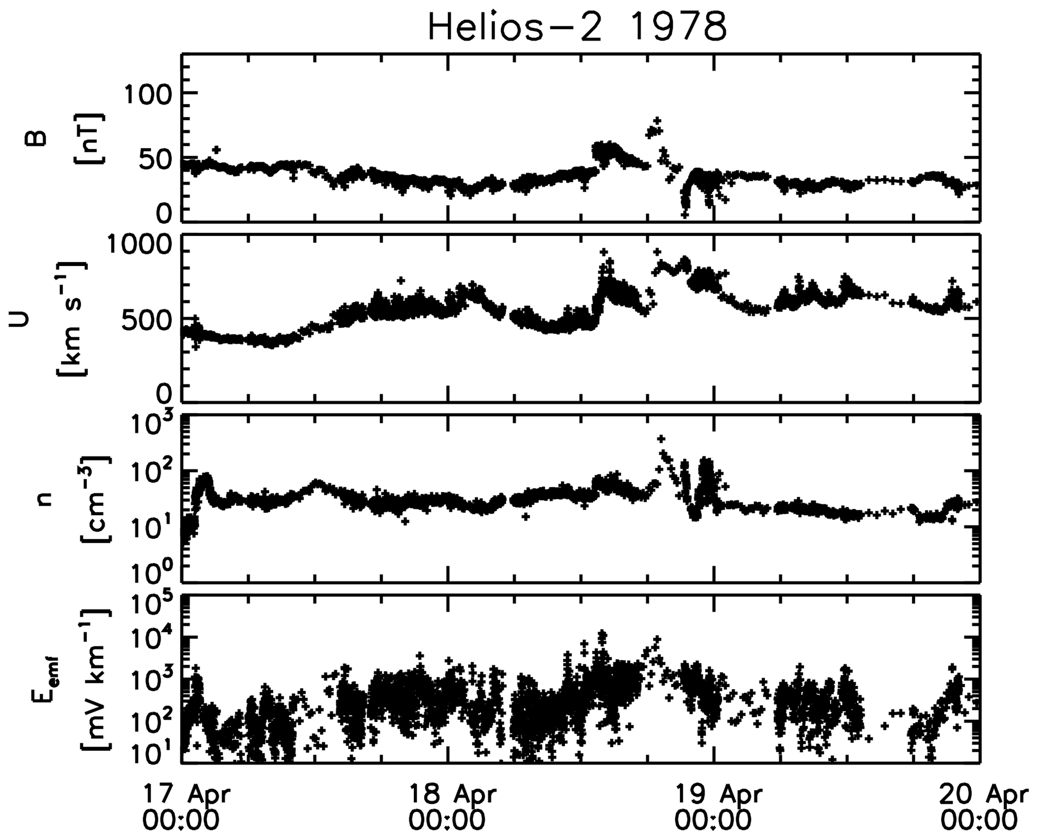
Figure 1Time series plots of magnetic field magnitude, flow velocity, proton number density, and instantaneous electromotive force (without statistical averaging or smoothing) obtained by Helios-2 spacecraft. Note a magnetic cloud or shock crossing at about 18:00–19:00 UT on 19 April 1978. Figure is produced using the data after Narita and Vörös (2018).
3.2 Spectral feature
The electromotive force has nearly random fluctuations as shown in Fig. 1, but the fluctuations are not Gaussian but rather exhibit a turbulence-like power-law energy spectrum. Figure 2 exhibits a spectrum of the out-of-ecliptic component of electromotive force Eemf,z as a function of the spacecraft-frame frequencies after Marsch and Tu (1992, 1993). The magnetic field and ion data obtained by the Helios-1 spacecraft at a distance of about 0.53 au in 1980 are used to compute the electromotive force spectrum.
The solar wind speed is about 637 km s−1 on the analyzed time interval, and the fluctuations are highly Alfvénic (with the components propagating away from the Sun dominating the fluctuations); the energy spectrum is close to Kolmogorov's inertial-range spectrum with a slope of . The frequency spectrum may thus be regarded as a nearly streamwise wavenumber spectrum when Taylor's frozen-in flow hypothesis is used. The electromotive force vanishes in the purely Alfvénic fluctuations, since the fluctuating flow velocity is either positively or negatively correlated to the fluctuating magnetic field. The overall power-law spectral formation is indicative of some turbulent cascade mechanism operating in the electromotive force.
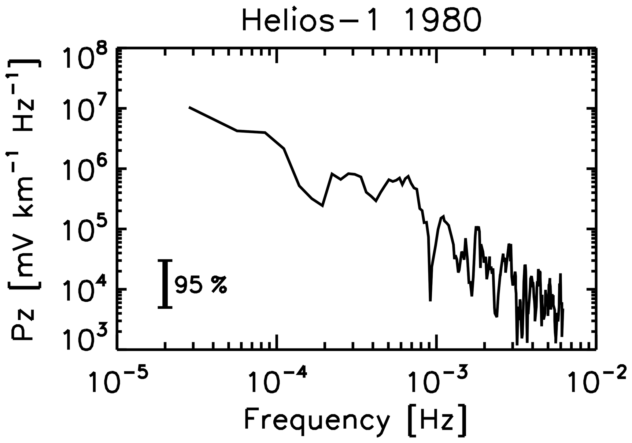
Figure 2Frequency spectrum (in the spacecraft frame) of the out-of-ecliptic component (the z component) of electromotive force derived from the Helios-1 at a radial distance of 0.53 astronomical units, after the spectral data presented by Marsch and Tu (1992). The magnitude value of the electromotive force is plotted here.
3.3 Observational tests
3.3.1 Test for the α effect
The validity of mean-field model can be tested against solar wind data in various ways. Marsch and Tu (1992) regarded the mean field model as a Taylor expansion with respect to the mean magnetic field 〈B〉 as the leading order and its spatial gradients (or curl of mean magnetic field) ∇×〈B〉 as higher-order terms. If the large-scale current is in the direction to the mean magnetic field (force-free configuration for the large-scale fields), and if the cross helicity term (with the coefficient γ) is negligible, the electromotive force is proportional to the mean magnetic field:
The simplified model (Eq. 15) is tested against the Helios-2 observation of fast solar wind near 0.29 au in 1976. Figure 3 displays a scatterplot of the electromotive force as a function of the mean magnetic field for three components: radially outward direction from the Sun (the x component) with plus signs in black, azimuthally westward direction (the y component) with asterisk symbols in dark gray, and solar-ecliptic north direction (the z component) with diamond symbols in light gray.
The α effect test result (Fig. 3) shows that no clear correlation is observed between the electromotive force and the mean magnetic field. The scatter is larger in the electromotive force than that in the mean field.
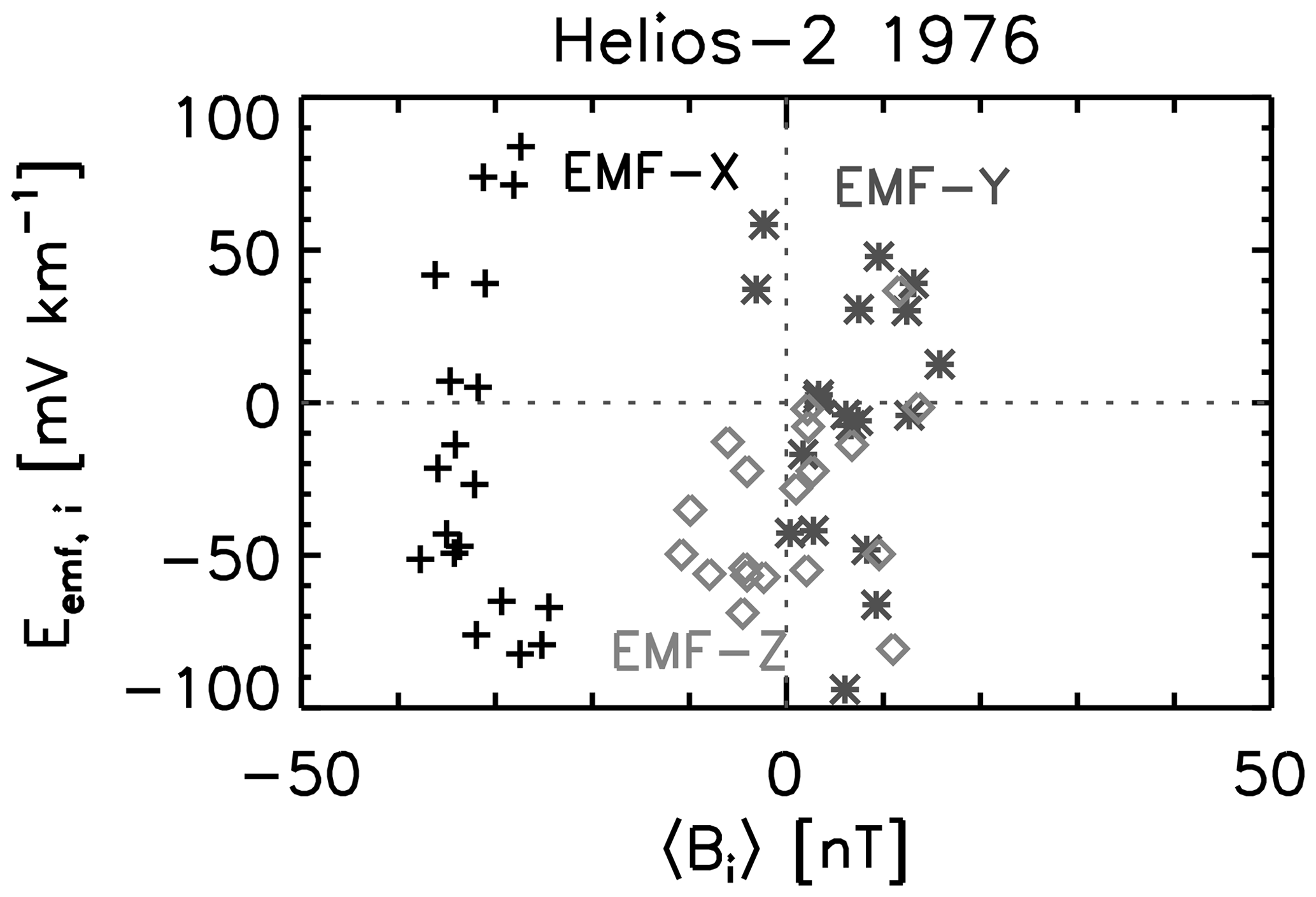
Figure 3Test for the α effect by plotting the electromotive force Eemf as a function of the mean magnetic field 〈B〉 using the Helios-2 solar wind data near perihelion (0.29 au from the Sun) in 1976. The x component (EMF-X) is radially away from the Sun, the y component (EMF-Y) is azimuthally westward (with respect to the ecliptic north), and the z component (EMF-Z) is northward to the ecliptic plane. Figure is produced using the data set presented by Marsch and Tu (1992).
3.3.2 Evaluation of the α and β coefficients
For the simple model with the α and β terms (indicating the field amplification and the turbulent diffusion, respectively), analytic forms are proposed to estimate the transport coefficients α and β (Narita and Vörös, 2018). For this purpose we model the electromotive force in the following form:
Vector product between the mean magnetic field 〈B〉 and the electromotive force Eemf in Eq. (16) yields
which can be arranged into an estimator for the β coefficient as
Here, F denotes the Lorentz force for the large-scale magnetic field and is defined as (by setting the permeability of free space μ0 to unity for simplicity)
For the coefficient α we multiply Eq. (16) by the mean magnetic field 〈B〉 and obtain the following:
Equation (20) can be arranged into
by using the estimator for the coefficient β (Eq. 18) and introducing the large-scale current helicity density hcrt as
The coefficients α and β are evaluated observationally using Eqs. (18) and (21), and they are graphically plotted as functions of the fluctuating flow speed and fluctuating magnetic field on the logarithmic scale in Fig. 4. The coefficients α and β exhibit the following properties:
-
Both the coefficients are scattered to a larger extent over the flow speed fluctuation u and the magnetic field fluctuation b. Variation of the coefficient α spans from 10−4 to 104 km s−1 (8 orders of magnitude), and that of β spans from 106 to 1016 km2 s−1 (10 orders of magnitude).
-
Yet, both the coefficients show a systematic trend that the values of coefficients increase at larger fluctuation amplitudes. The systematic trend appears not only in the flow speed domain (left panels) but also in the magnetic field domain (right panels). The systematic trend may as well be (observationally) modeled using a power-law scaling (linearly on the logarithmic scale).
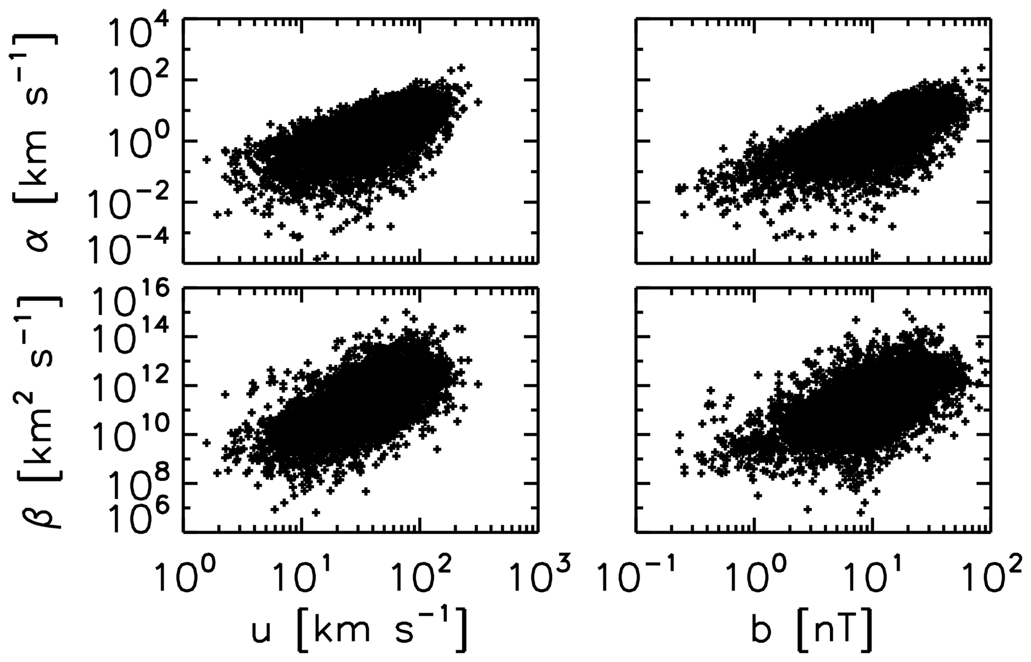
Figure 4Transport coefficients α and β as functions of the fluctuating flow speed and fluctuating magnetic field for the two-component electromotive force model with the α and β terms. The Helios solar wind data and the transport coefficients studied by Narita and Vörös (2018) are used for the graphics.
3.3.3 Test for the mean-field model
The electromotive force can be evaluated by directly computing the cross product between the fluctuating flow velocity and the fluctuating magnetic field after Eq. (1) and also by making use of the mean-field model with the helical dynamo term (the α term), the magnetic diffusion term (the β term), and the cross helicity dynamo term (the γ term) after Eq. (5). By doing so, it is possible to validate the mean-field model using in situ plasma and magnetic field measurements in the solar wind.
Figure 5 displays the time series plot of electromotive force using the Helios-2 observation of magnetic cloud (or shock crossing) event on 18 April 1976 (the same event as shown in Fig. 1). The electromotive force is then computed with Eq. (5) by estimating the kinetic helicity, magnetic fluctuation energy, and cross helicity, and turbulence correlation time (shown by the curve in gray). Though not exact, the mean-field model can qualitatively reproduce the observationally determined electromotive force in the sense that both the peak time and the peak value are in good agreement.
It is interesting to note that the test for the single α effect (i.e., proportionality of electromotive force solely to the mean magnetic field without the β and the γ effects) fails against the solar wind data after Marsch and Tu (1992), yet the test for the model with the three terms including the α, β, and γ terms successfully reproduces the measured electromotive force after Bourdin et al. (2018). The scaling analysis using Eq. (23) indicates that the α term should be almost as important as the β term (in fact, 4 times larger), which is as important as the γ term. Hence, the lesson is that the simplest model using only the α term is not sufficient and that the magnetic diffusion and the cross helicity effect should be considered as well in the electromotive force composition. Under which conditions the α effect will dominate remains an observationally open question; perhaps there is a dependence on, e.g., fast or slow solar wind, quieter or more disturbed solar wind, association with transient events such as coronal mass ejections and corotating interaction regions.
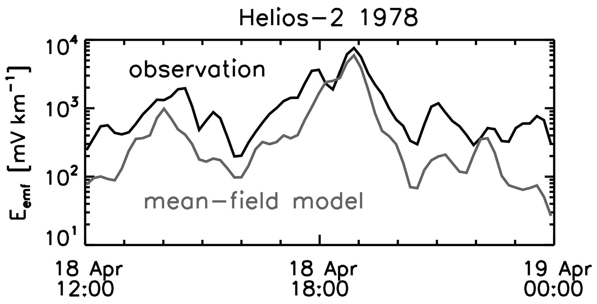
Figure 5Comparison of the electromotive force magnitude computed from the Helios-2 of plasma and magnetic field fluctuation data (in black) and that from the mean-field model using the Helios-2 mean field data (in gray) for the shock crossing event on 18 April 1978 (the same event as that in Fig. 1). Figure is produced using the data in Bourdin et al. (2018).
It is interesting to compare the three terms in the electromotive force model (α term, β term, and γ term) in Eq. (5) using the order-of-magnitude estimate method. The reconstruction work by Bourdin et al. (2018) determined the values of coefficients α, β, and γ as shown in Table 1.
Table 1Transport coefficients estimated from a 12 h solar wind interval including an interplanetary shock (active solar wind) and a quasi-stationary turbulent state (quiet solar wind) after Bourdin et al. (2018).
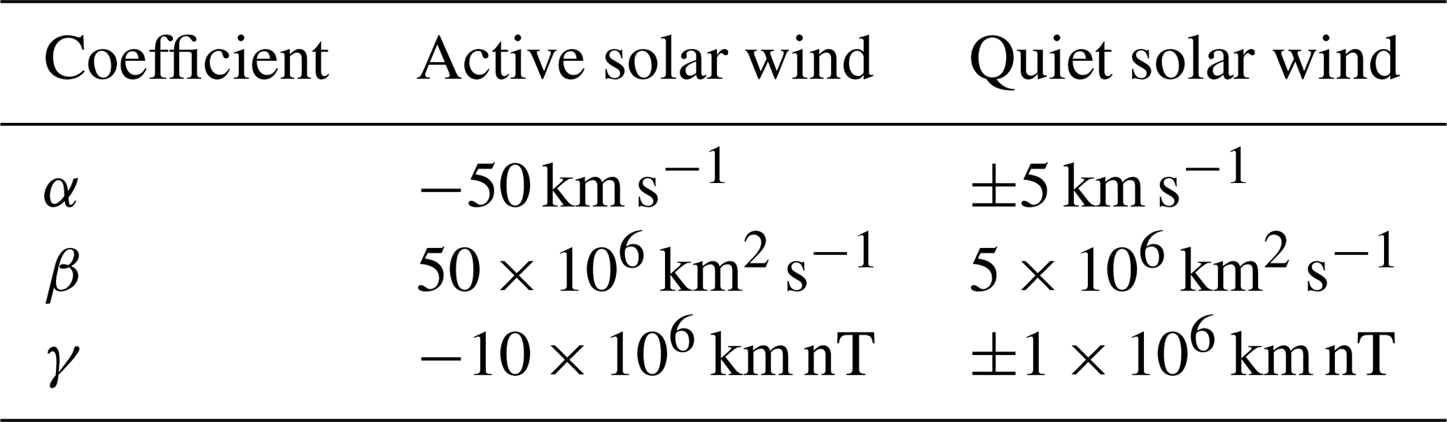
The ratio of the α term (helical dynamo term) to the β term (turbulent diffusion term) is estimated nearly of the order of unity:
where the spatial gradient scale is estimated about km in the solar wind corresponding to a Doppler-shifted frequency of about 104 Hz (e.g., Tu and Marsch, 1995). The order-of-unity estimate as in Eq. (23) is valid for both the active solar wind and the quiet solar wind when referring to the observational values of the transport coefficients in Table 1. The ratio of the γ term (cross helicity term) to the β term is estimated of the order of unity, too:
Here we used a flow speed of U0=400 km s−1 (typical both in the inner heliosphere and around the Earth orbit) and a magnetic field of B0=40 nT (typical in the inner heliosphere but not around the Earth). The cross helicity term plays a more important role because the flow speed does not change very much over the radial distances from the Sun while the magnetic field decays radially due to the flux conservation over the spatial expansion. Around the Earth orbit, the ratio of the γ term to the β term is expected to be about 10 times larger than that in the inner heliosphere.
3.4 Radial evolution in the heliosphere
The electromotive force becomes enhanced during shock crossings, reaching the order of 1 V km−1. The spatial distribution or the radial profile of electromotive force during the shock crossings is determined using the whole Helios data in the inner heliosphere down to the perihelion of about 0.29 astronomical units. A shock detection algorithm was developed using the electromotive force, and the algorithm was applied to the whole Helios data to identify 531 shock crossing events (Hofer and Bourdin, 2019).
Figure 6 displays a scatterplot of electromotive force during the shock crossings as a function of the radial distance of observation from the Sun. The shock-enhanced electromotive force tends to decay at larger distances from the Sun. The electromotive force is 1–10 V km−1 near the perihelion (0.29 au) and decays to 0.1–10 V km−1 near the aphelion (close to 1 astronomical unit). The spatial decay or radial decay of electromotive force can in practice be fitted by a power-law curve as r−1.54 (Hofer and Bourdin, 2019).
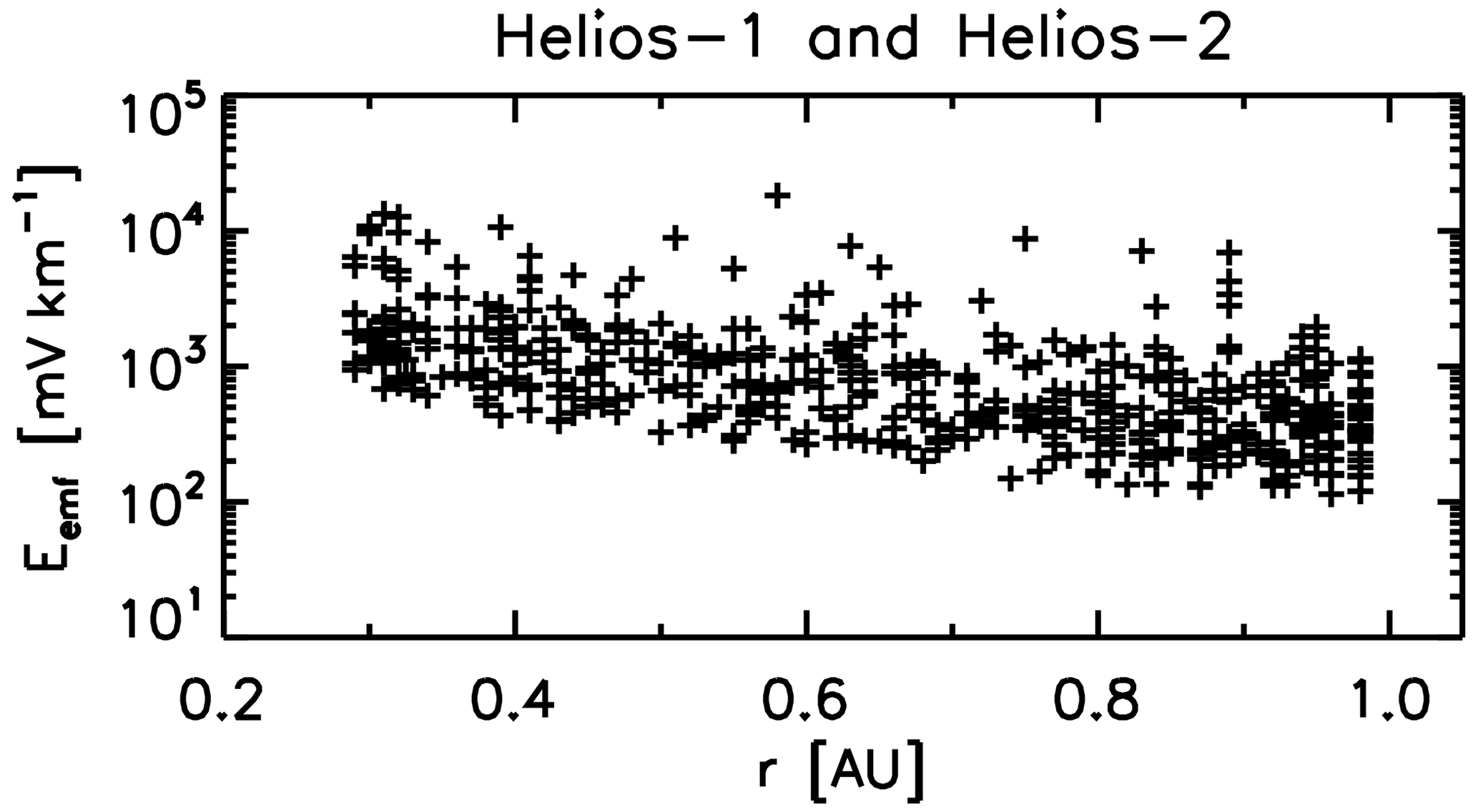
Figure 6Distribution of peak values of electromotive force (as a magnitude) as a function of radial distance from the Sun for shock crossing events in the Helios-1 and Helios-2 data. Figure is produced using the data in Hofer and Bourdin (2019).
The electromotive force has largely been overlooked in space plasma studies in contrast to the conventional turbulence analysis methods such as energy spectra and helicity profiles. The electromotive force is one of the second-order fluctuation quantities (cf. the Reynolds stress tensors in fluid dynamics). Though the number of studies is limited, the properties of electromotive force are determined using the Helios spacecraft data in the inner heliosphere. To summarize, the properties are the following:
-
The electromotive force is non-zero even in the quiet solar wind. Its magnitude is of the order of 1 or 10 mV km−1 in the quiet solar wind, corresponding to the fluctuating flow velocity of 1 km s−1 and the fluctuating magnetic field of 1 nT, and can reach the order of 1 or 10 V km−1 during the magnetic clouds or shock crossings.
-
The fluctuations of electromotive force are nearly random, and the spectrum (in the spacecraft-frame frequency domain) represents a power-law curve with a slope close to .
-
The mean-field model of electromotive force can be tested against the Helios data. The proportionality does not hold between the electromotive force and the α effect, but together with the magnetic diffusion (β term) and the cross helicity effect (γ term) the electromotive force can qualitatively be reconstructed using the large-scale magnetic field and flow velocity.
-
The electromotive force during the shock crossings decays as a function of the radial distance from the Sun, from 1–10 V km−1 at a distance of 0.3 au down to 0.1–1 V km−1.
Local magnetic field amplification is possible in the solar wind and is associated with the electromotive force (in particular, the α and cross helicity effects). Crossing of coronal mass ejections or transient events or wake region behind obstacles such as planets or other solar system bodies (asteroids, satellites, and comets) may be potential regions of interest for testing for non-zero electromotive force.
Statistical behavior of turbulent fields is more complete when the electromotive force is properly assessed or modeled in addition to the energy densities (for the magnetic field and the flow velocity) and helicity quantities (for the cross helicity, current helicity, and kinetic helicity). It is important to note here that the construction of mean field and identification of fluctuating fields is not unique. The mean field is determined by smoothing (e.g., running average), a local filter (boxcar, Gaussian), and a low-pass filter. Since solar wind turbulence has fluctuations on various spatial and temporal scales, the magnitude of electromotive force may likely depend on the averaging process such as coarse graining.
The electromotive force can serve as a data analysis tool. Hofer and Bourdin (2019) proposed a classification scheme for the shock crossings into the jump type (e.g., coronal mass ejections) and the transient type (e.g., co-rotating interaction regions). Various types of discontinuities or structures may be better identified using the electromotive force, for example, shock types (fast, slow, and intermediate shocks), magnetic reconnection exhausts, and detailed structures within the current sheets and shocks.
Energy densities, helicity densities, and electromotive force are the second-order fluctuation quantities using the magnetic field and flow velocity. The energy density of fluctuating magnetic field is
The kinetic energy density is
where ρ is the mass density of medium.
The cross helicity density is a correlation between the magnetic field and the flow velocity,
The current helicity density is
Note that the helicity in general (e.g., magnetic helicity density and current helicity) is non-zero when the field is helical, e.g., when choosing the left-handed (or right-handed) helical field around the mean field B0 in the z direction,
where the plus sign is for the left-hand helical field when tracking the field rotation sense along the wave vector in the z direction k, and the minus sign for the right-hand helical field, respectively. δb denotes the amplitude of the helical rotation. The magnetic helicity density can also be constructed from the fluctuating magnetic field by un-curling the vector potential in the Fourier domain under the Coulomb gauge as
The kinetic helicity density is constructed as
and the electromotive force is
From a data-analysis point of view, the second-order quantities introduced above can be derived from the correlation matrices (or spectral density matrices when working in the spectral domain):
The magnetic and kinetic energy densities correspond to the diagonal elements of Mbb and Muu, respectively. The cross helicity density is derived from the diagonal elements of Mub. The current and kinetic helicity densities are constructed from the off-diagonal elements of Mbb and Muu, respectively. The electromotive force is constructed from the off-diagonal elements of Mub. The Reynolds stress tensors for magnetohydrodynamic turbulence are constructed as for the kinetic variant and for the magnetic variant (Yoshizawa, 1990).
Helios data are available at CDAWeb https://cdaweb.sci.gsfc.nasa.gov (NASA Coordinated Data Analysis Web, 2021).
The author declares that there is no conflict of interest.
Publisher’s note: Copernicus Publications remains neutral with regard to jurisdictional claims in published maps and institutional affiliations.
The author thanks many colleagues for stimulating discussions and providing data and materials on the concept of electromotive force: Philippe-A. Bourdin, Iver Cains, Abraham Chian, Tohru Hada, Bernhard Hofer, Gurbax Lakhina, Eckart Marsch, Donald Melrose, and Nobumitsu Yokoi.
This research has been supported by the Austrian Research Promotion Agency (FFG) (grant no. 865967).
This paper was edited by Anna Milillo and reviewed by two anonymous referees.
Beck, R., Chamandy, L., Elson, E., and Blackman, E. G.: Synthesizing observations and theory to understand galactic magnetic fields: Progress and challenges, Galaxies, 8, 4, https://doi.org/10.3390/galaxies8010004, 2020. a
Benkhoff, J., van Casteren, J., Hayakawa, H., Fujimoto, M., Laakso, H., Novara, M., Ferri, P., Middleton, H. R., and Ziethe, R.: BepiColombo – Comprehensive exploration of Mercury: Mission overview and science goals, Planet. Space Sci., 58, 2–20, https://doi.org/10.1016/j.pss.2009.09.020, 2010. a
Berdyugina, S. V.: Starspots: A key to the stellar dynamo, Liv. Rev. Sol. Phys., 2, 8, https://doi.org/10.12942/lrsp-2005-8, 2005. a
Berger, M. A.: Introduction to magnetic helicity, Plasma Phys. Control. Fusion, 41, B167–B175, https://doi.org/10.1088/0741-3335/41/12B/312, 1999. a
Berger, M. A. and Field, G. B.: The topological properties of magnetic helicity, J. Fluid Mech., 147, 133–148, https://doi.org/10.1017/S0022112084002019, 1984. a
Bourdin, Ph.-A., Hofer, B., and Narita Y.: Inner structure of CME shock fronts revealed by the electromotive force and turbulent transport coefficients in Helios-2 observations, Astrophys. J., 855, 111, https://doi.org/10.3847/1538-4357/aaae04, 2018. a, b, c, d, e, f
Brandenburg, A.: Advances in mean-field dynamo theory and applications to astrophysical turbulence, J. Plasma Phys., 84, 735840404, https://doi.org/10.1017/S0022377818000806, 2018. a, b
Brun, A. S. and Browning, M. K.: Magnetism, dynamo action and the solar-stellar connection, Liv. Rev. Sol. Phys., 14, 4, https://doi.org/10.1007/s41116-017-0007-8, 2017. a
Charbonneau, P.: Dynamo models of the solar cycle, Liv. Rev. Sol. Phys., 7, 3, https://doi.org/10.12942/lrsp-2010-3, 2010. a
Charbonneau, P.: Solar dynamo theory, Annu. Rev. Astron. Astrophys., 52, 251–290, https://doi.org/10.1146/annurev-astro-081913-040012, 2014. a
Elsasser, W. M.: Hydromagnetic dynamo theory, Rev. Mod. Phys., 28, 135–163, https://doi.org/10.1103/RevModPhys.28.135, 1956. a
Fox, N. J., Velli, M. C., Bale, S. D., Deckert, R., Driesman, A., Howard, R. A., Kasper, J. C., Kinnison, J., Kusterer, M., Lario, D., Lockwood, M. K., McComas, D. J., Raouafi, N. E., and Szabo, A.: The Solar Probe Plus mission: Humanity’s first visit to our star, Space Sci. Rev., 204, 7–48, https://doi.org/10.1007/s11214-015-0211-6, 2016. a
Glatzmaier, G. A.: Geodynamo simulations – How realistic are they?, Annu. Rev. Earth Pl. Sc., 30, 237–257, https://doi.org/10.1146/annurev.earth.30.091201.140817, 2002. a
Glatzmaier, G. A. and Roberts, P. H.: Dynamo theory then and now, Int. J. Eng. Sci., 36, 1325–1338, https://doi.org/10.1016/S0020-7225(98)00035-4, 1998. a
Hamba, F.: Turbulent dynamo effect and cross helicity in magnetohydrodynamic flows, Phys. Fluid. A, 4, 441–450, https://doi.org/10.1063/1.858314, 1992. a
Hofer, B., and Bourdin, Ph.-A.: Application of the electromotive force as a shock front indicator in the inner heliosphere, Astrophys. J., 878, 30, https://doi.org/10.3847/1538-4357/ab1e48, 2019. a, b, c, d, e
Jones, C. A.: Planetary magnetic fields and fluid dynamocs, Annu. Rev. Fluid Mech., 43, 583–614, https://doi.org/10.1146/annurev-fluid-122109-160727, 2011. a
Kono, M. and Roberts, P. H.: Recent geodynamo simulations and observations of the geomagnetic field, Rev. Geophys., 40, 4, https://doi.org/10.1029/2000RG000102, 2002. a
Krause, F. and Rädler, K.-H.: Mean-field Magnetohydrodynamics and Dynamo Theory, Pergamon, Oxford, 1980. a
Kronberg, P. P.: Extragalactic magnetic fields, Rep. Prog. Phys. 57, 325–382, https://doi.org/10.1088/0034-4885/57/4/001, 1994. a
Mangano, V., Dósa, M., Fränz, M., Milillo, A., Oliveira, J. S., Lee, Y. J., McKenna-Lawlor, S., Grassi, D., Heyner, D., Kozyrev, A. S., Peron, R., Helbert, J., Besse, S., de la Fuente, S., Mongagnon, E., Zender, J., Volwerk, M., Chaufray, J.-Y., Slavin, J. A., Krüger, H., Maturilli, A., Cornet, T., Iwai, K., Miyoshi, Y., Lucente, M., Massetti, S., Schmidt, C. A., Dong, C., Quarati, F., Hirai, T., Varsani, A., Beyaev, D., Zhong, J., Kilpua, E. K. J., Jackson, B. V., Odstrcil, D., Plaschke, F., Vainio, R., Jarvinen, R., Ivanovski, S. L., Madár, Á., Erdős, G., Plainaki, C., Alberti, T., Aizawa, S., Benkhoff, J., Murakami, G., Quemerais, E., Hiesinger, H., Mitrofanov, I. G., Iess, L., Santoli, F., Orsini, S., Lichtenegger, H., Laky, G., Barabash, S., Moissl, R., Huovelin, J., Kasaba, Y., Saito, Y., Kobayashi, M., and Baumjohann, W.: BepiColombo science investigations during cruise and flybys at the Earth, Venus and Mercury, Space Sci. Rev., 217, 23, https://doi.org/10.1007/s11214-021-00797-9, 2021. a
Marsch, E. and Tu, C.-Y.: Electric field fluctuations and possible dynamo effects in the solar wind, Solar Wind Seven, Proceedings of the 3rd COSPAR Colloquium, Goslar, Germany, 16–20 September 1991, edited by: Marsch, E. and Schwenn, R., Pergamonn Press, Oxford, 505–510, https://doi.org/10.1016/B978-0-08-042049-3.50105-8, 1992. a, b, c, d, e, f
Marsch, E. and Tu, C.-Y.: MHD turbulence in the solar wind and interplanetary dynamo effects, The Cosmic Dynamo, Proceedings of the 157th Symposium of the International Astronomical Union held in Potsdam, Germany, 7–11 September 1992, edited by: Krause, F., Rädler, K.-H., and Rüdiger, G., International Astronomical Union, Springer, Dordrecht, 51–57, https://doi.org/10.1007/978-94-011-0772-3_9, 1993. a, b
Matthaeus, W. H., Goldstein, M. L., and Smith, C.: Evaluation of magnetic helicity in homogeneous turbulence, Phys. Rev. Lett., 48, 1256–1259, https://doi.org/10.1103/PhysRevLett.48.1256, 1982. a
Moffatt, H. K.: Magnetic Field Generation in Electrically Conducting Fluids, Cambridge University Press, Cambridge, 1978. a
Moffatt, H. K.: Helicity and singular structures in fluid dynamics, P. Natl. Acad. Sci. USA, 111, 3663–3670, https://doi.org/10.1073/pnas.1400277111, 2014. a
Müller, D., St. Cyr, O. C., Zouganelis, I., Gilbert, H. R., Marsden, R., Nieves-Chinchilla, T., Antonucci, E., Auchère, F., Berghmans, D., Horbury, T. S., Howard, R. A., Krucker, S., Maksimovic, M., Owen, C. J., Rochus, P, Rodriguez-Pacheco, J., Romoli, M., Solanki, S. K., Bruno, R., Carlsson, M., Fludra, A., Harra, L., Hassler, M., Livi, S., Louarn, P., Peter, H., Schühle, U., Teriaca, L., del Toro Iniesta, J. C., Wimmer-Schweingruber, R. F., Marsch, E., Velli, M., De Groof, A., Walsh, A., and Williams, D.: The Solar Orbiter mission, Astron. Astrophys., 642, A1, https://doi.org/10.1051/0004-6361/202038467, 2020. a
Narita, Y. and Vörös, Z.: Evaluation of electromotive force in interplanetary space, Ann. Geophys., 36, 101–106, https://doi.org/10.5194/angeo-36-101-2018, 2018. a, b, c, d
NASA Coordinated Data Analysis Web (CDAWeb): Helios data, CDAWeb [data set], available at: https://cdaweb.gsfc.nasa.gov, last access: 18 August 2021. a
Pouquet, A., Frisch, U., and Léorat, J.: Strong MHD helical turbulence and the nonlinear dynamo effect, J. Fluid Mech., 77, 321–354, https://doi.org/10.1017/S0022112076002140, 1976. a, b
Roberts, P. and Glatzmaier, G. A.: Geodynamo theory and simulations, Rev. Mod. Phys., 72, 1081–1123, https://doi.org/10.1103/RevModPhys.72.1081, 2000. a
Roberts, P. H. and Soward, A. M.: Dynamo theory, Ann. Rev. Fluid Mech., 24, 459–512, https://doi.org/10.1146/annurev.fl.24.010192.002331, 1992. a
Sarson, G. R., Jones, C. A., Zhang, K., and Schubert, G.: Magnetoconvection dynamos and the magnetic fields of Io and Ganumede, Science, 276, 1106–1108, https://doi.org/10.1126/science.276.5315.1106, 1997. a
Schubert, G., Zhang, K., Kivelson, M. G., and Anderson, J. D.: The magnetic field and internal structure of Ganymede, Nature, 384, 544–545, https://doi.org/10.1038/384544a0, 1996. a
Steenbeck, M., Krause, F., and Rädler, K.-H.: Berechnung der mittleren Lorentz-Feldstärke für ein elektrisch leitendes Medium in turbulenter, durch Coriolis-Kräfte beeinflußter Bewegung, Z. Naturforsch., 21a, 369–376, https://doi.org/10.1515/zna-1966-0401, 1966. a
Tu, C.-Y. and Marsch, E.: MHD structures, waves and turbulence in the solar wind: Observations and theories, Space Sci. Rev., 73, 1–210, 1995. a
Vainshtein, S. I. and Ruzmaikin, A. A.: Generation of the large-scale galactic magnetic field, Astron. Z., 48, 902–909, 1971 (English translation in Sov. Astron. AJ, 15, 714–719, 1972). a
Widrow, L. M.: Origin of galactic and extragalactic magnetic fields, Rev. Mod. Phys., 74, 775–823, https://doi.org/10.1103/RevModPhys.74.775, 2002. a
Yokoi, N.: Cross helicity and related dynamo, Geophys. Astrophys. Fluid Dyn., 107, 114–184, https://doi.org/10.1080/03091929.2012.754022, 2013. a, b
Yokoi, N.: Electromotive force in strongly compressible magnetohydrodynamic turbulence, J. Plasma Phys., 84, 735840501, https://doi.org/10.1017/S0022377818000727, 2018a. a
Yokoi, N.: Turbulent dynamos beyond the heuristic modelling: Helicities and density variance, AIP Conf. Proc., 1993. 020010, https://doi.org/10.1063/1.5048720, 2018b. a
Yokoi, N. and Balarac, G.: Cross-helicity effects and turbulent transport in magnetohydrodyamic flow, J. Phys. Conf. Ser., 318, 072039, https://doi.org/10.1088/1742-6596/318/7/072039, 2011. a
Yoshizawa, A: Self-consistent turbulent dynamo modeling of reversed field pinches and planetary magnetic fields, Phys. Fluids B, 2, 1589–1600, https://doi.org/10.1063/1.859484, 1990. a, b
Yoshizawa, A.: Hydrodynamic and Magnetohydrodynamic Turbulent Flows: Modelling and Statistical Theory, Kluwer Academic Publishers, Dordrecht, 1998. a