the Creative Commons Attribution 4.0 License.
the Creative Commons Attribution 4.0 License.
 | 29 Jul 2021
Steepening of magnetosonic waves in the inner coma of comet 67P/Churyumov–Gerasimenko
Katharina Ostaszewski
Karl-Heinz Glassmeier
Charlotte Goetz
Philip Heinisch
Pierre Henri
Sang A. Park
Hendrik Ranocha
Ingo Richter
Martin Rubin
Bruce Tsurutani
We present a statistical survey of large-amplitude, asymmetric plasma and magnetic field enhancements detected outside the diamagnetic cavity at comet 67P/Churyumov–Gerasimenko from December 2014 to June 2016. Based on the concurrent observations of plasma and magnetic field enhancements, we interpret them to be magnetosonic waves. The aim is to provide a general overview of these waves' properties over the mission duration. As the first mission of its kind, the ESA Rosetta mission was able to study the plasma properties of the inner coma for a prolonged time and during different stages of activity. This enables us to study the temporal evolution of these waves and their characteristics. In total, we identified ∼ 70 000 steepened waves in the magnetic field data by means of machine learning. We observe that the occurrence of these steepened waves is linked to the activity of the comet, where steepened waves are primarily observed at high outgassing rates. No clear indications of a relationship between the occurrence rate and solar wind conditions were found. The waves are found to propagate predominantly perpendicular to the background magnetic field, which indicates their compressional nature. Characteristics like amplitude, skewness, and width of the waves were extracted by fitting a skew normal distribution to the magnetic field magnitude of individual steepened waves. With increasing mass loading, the average amplitude of the waves decreases, while the skewness increases. Using a modified 1D magnetohydrodynamic (MHD) model, we investigated if the waves can be described by the combination of nonlinear and dissipative effects. By combining the model with observations of amplitude, width and skewness, we obtain an estimate of the effective plasma diffusivity in the comet–solar wind interaction region and compare it with suitable reference values as a consistency check. At 67P/Churyumov–Gerasimenko, these steepened waves are of particular importance as they dominate the innermost interaction region for intermediate to high activity.
- Article
(4431 KB) - Full-text XML
-
Supplement
(218 KB) - BibTeX
- EndNote


The groundbreaking ESA Rosetta mission (Glassmeier et al., 2007a; Taylor et al., 2017; Glassmeier, 2017) was the first of its kind to orbit a comet and study its plasma environment over a prolonged time of about 2 years. As a comet approaches the Sun, insolation leads to the sublimation of ices. The emanated neutral gas is subsequently ionized, which triggers the formation of an interaction region, including boundaries and structures such as a bow shock (Koenders et al., 2013, 2015) and a diamagnetic cavity (Goetz et al., 2016a). Due to changing solar wind conditions and variability in the outgassing, the interaction region is highly dynamical in nature. Facilitated by the comparatively long duration, the Rosetta mission provides unprecedented possibilities to observe the evolution of the cometary plasma, with special emphasis on changing cometary activity and solar wind conditions. Due to its operational design, Rosetta was primarily located in the innermost interaction region. There, one of the most striking features observed are large-amplitude, asymmetric plasma enhancements, which have been observed inside and outside the diamagnetic cavity (Stenberg Wieser et al., 2017; Engelhardt et al., 2018; Hajra et al., 2018b). Although the plasma pulses inside and outside of the diamagnetic cavity are similar in shape (Engelhardt et al., 2018; Hajra et al., 2018b), they must be of different nature because those detected outside the cavity have strong magnetic components. Those plasma pulses inside the diamagnetic cavity are devoid of magnetic signatures as defined by the term diamagnetic cavity, where no substantial magnetic fields are detected. Hajra et al. (2018b) mention the hypothesis that external magnetosonic waves propagating inward to the cavity boundary are producing the interior plasma pulses by their interaction with the cavity boundary. However, the authors also mention that there is not enough observational evidence to support this hypothesis. In this study, we will focus on the properties of the magnetic pulses outside of the cavity. Because it has already been shown by Stenberg Wieser et al. (2017), Hajra et al. (2018b) and Engelhardt et al. (2018) that the magnetic pulses occur simultaneously with plasma pulses, we interpret these as magnetosonic waves.
Figure 1 shows two exemplary intervals with multiple occurrences of these waves in the magnetic field data and electron density on 16 July 2015 and 21 November 2015. During both intervals, the outgassing rate was already high enough to facilitate the development of a diamagnetic cavity (Goetz et al., 2016a, b) and, with a high probability, a bow shock (Koenders et al., 2013, 2015). The striking features of Fig. 1 are the asymmetric, large-amplitude enhancements in the magnetic field and electron density. While properties like amplitude, width and strength of asymmetry can change significantly from steepened wave to steepened wave, they are still strikingly similar in respect to their general shape. In particular, for all instances of magnetic field enhancements, concurrent enhancements in the electron density are visible.

Figure 1Magnetic field magnitude (a, b), electron density (c, d) and magnetic field components (e, f), with multiple occurrences of concurrent magnetic field and density enhancements on 16 July and 21 November 2015.
Since the simultaneous occurrence of magnetic field and electron density enhancements (Engelhardt et al., 2018) leads to a pressure imbalance, these structures will either propagate as waves or they will disperse. The waves shown in Fig. 1 also resemble compressional nonlinear phase-steepened waves, which have been previously observed at planetary foreshocks and comets. At Earth, the foreshock region has been crossed multiple times by various spacecrafts, which facilitates extensive statistical studies of nonlinear waves (Tsurutani and Rodriguez, 1981; Schwartz et al., 1992; Giacalone et al., 1993; Mann et al., 1994; Stasiewicz et al., 2003; Behlke et al., 2004; Lucek et al., 2004). Similarly, nonlinear waves were recently studied in great detail at Mars, where the Maven mission provided high-resolution measurements of magnetic fields and particle properties (Fowler et al., 2018; Shan et al., 2020). In contrast to planetary missions, cometary missions previous to Rosetta were exclusively fast flybys or impacts, which only provided limited information on the properties of nonlinear waves for a fixed cometary activity level. First observations of nonlinear waves at comets were obtained by the International Cometary Explorer (ICE) at 21P/Giacobini–Zinner (Smith et al., 1986). Tsurutani and Smith (1986) report indications of high-intensity turbulence, which is mainly characterized by the presence of large-amplitude compressional waves. In the region far upstream of the bow shock, predominantly long-period elliptically polarized waves are present. With decreasing distance to the comet, Tsurutani et al. (1987) report steepening of fast-mode waves accompanied by high-frequency wave packets at the leading edge of the wave. In contrast to 21P/Giacobini–Zinner, where steepening occurred at the leading edge, steepening occurred at the trailing edge in the case of 26P/Grigg–Skjellerup (Neubauer et al., 1993; Tsurutani et al., 1995). A comprehensive review of low-frequency waves at comets is given by, e.g., Glassmeier et al. (1997). As source mechanisms for these waves, ion ring-beam instabilities (Wu and Davidson, 1972) and nongyrotropic phase space density-driven instabilities (Motschmann and Glassmeier, 1993) were proposed. Depending on the angle between the interplanetary magnetic field BIMF and the solar wind flow usw, newborn cometary ions form ring, ring-beam or beam distributions in velocity space. In general, these distributions are unstable in relation to resonant wave growth (Sagdeev et al., 1986; Gary, 1991). A full ring-beam distribution is only formed if cometary ions are produced over lengths scales larger than the cometary ion gyroradius. If ionization takes place on smaller scales, the ring-beam distribution can only be partially filled, leading to a nongyrotropic distribution as observed at 26P/Grigg–Skjellerup. At 67P/Churyumov–Gerasimenko (67P/CG), a ring-beam distribution was expected at large distances from the comet during the strongly active months around perihelion. However, due to its operational design, Rosetta was primarily located in the innermost interaction region and, hence, never able to observe a bow shock crossing. Consequently, the existence of nonlinear waves near the bow shock region at 67P/CG is unconfirmed. Such low-frequency waves were also expected at lower outgassing rates but were never observed (Glassmeier, 2017). Instead, a new type of nonlinear low-frequency waves, often termed “singing comet” waves, was encountered (Richter et al., 2015). Since the characteristics of these waves did not fit a ring-beam instability, Richter et al. (2015) suggested a cross-field current instability as the possible source mechanism. Based on these observations, Meier et al. (2016) proposed a modified ion-Weibel instability.
The aim of this study is twofold. At first we present a comprehensive statistical analysis of the magnetic part of the waves as shown in Fig. 1 from December 2014 to June 2016. In a second part, we investigate the possibility that the observed magnetic field and plasma pulses are phase-steepened waves using a modified 1D magnetohydrodynamic (MHD) model to describe some of their properties. To achieve this, the paper is structured as follows. In Sect. 2, we provide details about instrumentation relevant for this study and the method used to select intervals of interest. Subsequently, the in situ observations of the waves are described and used to characterized the general properties of said structures in Sects. 3 to 6. In Sect. 7, we use a modified 1D MHD model with an initial wave-like disturbance to describe the observed waves as an interplay between nonlinear wave steepening and diffusive effects.
To probe the ambient plasma, the Rosetta spacecraft was equipped with a set of five instruments, the Rosetta Plasma Consortium (RPC; Carr et al., 2007), designed to monitor particle properties and electromagnetic fields at 67P/CG. The primary focus of this study is the analysis of asymmetric magnetic field enhancements, which were observed by RPC-MAG. The latter consists of two tri-axial fluxgate magnetometer mounted 15 cm apart from each other on a 1.5 m long boom (Glassmeier et al., 2007b). For the following analysis, only the outboard magnetometer data were used. However, the difference between the measured signal on the outboard and inboard magnetometer was used for quality assessment of the magnetic field measurements. If the difference exceeded 5 nT, the time interval was excluded from the analysis. The magnetometer can either be operated in burst mode (20 Hz) or in normal mode (1 Hz). Because of the transient nature of these magnetic field signatures, we have exclusively used data sampled with a frequency of 20 Hz. Intervals for which only 1 Hz data were available were excluded from the analysis. Additionally to the magnetic field, we use electron density data from the RPC Mutual Impedance Probe (RPC-MIP; Trotignon et al., 2007) and neutral gas densities obtained from the Rosetta Orbiter Spectrometer for Ion and Neutral Analysis (ROSINA; Balsiger et al., 2007) comet pressure sensor (ROSINA-COPS) at suitable times. For our analysis, we have processed measurements made between 1 December 2014 and 31 June 2016. In the time periods before and after our interval of interest, cometary activity was low, resulting in mostly undisturbed solar wind being observed at Rosetta.
In order to study the occurrence and properties of the asymmetric magnetic field enhancements, intervals of interest have to be identified in a first step. The Rosetta magnetic field data used for this study are made available through the PSA archive of ESA (Besse et al., 2018) and the PDS archive of NASA. Intervals of interest can be distinguished by the characteristic shape, in particular by the distinctly pronounced asymmetry, of the structures in the magnetic field magnitude. Due to the comparatively long mission duration and the resulting large data set, manual identification was found to be unfeasible. Hence, an automated approach using machine learning techniques was used instead (Ostaszewski et al., 2020). Due to their distinct shape and the comparatively large number of asymmetric enhancements, it was possible to train a neural network to detect possible candidates, with a high precision of around 80 %. Nevertheless, false detections still occurred and were removed by means of fitting according to the following sections. Because of differing sampling times between the RPC plasma instruments and limited data availability, only magnetic field data were used as input for the neural network. Hence, asymmetric density enhancements observed inside the diamagnetic cavity (Hajra et al., 2018b) are not taken into account in this study. For all identified intervals, for which plasma data were available, we have checked that the magnetic field enhancements occur concurrently with density enhancements. Hajra et al. (2018b) noted that the signature in the magnetic field of a diamagnetic boundary crossing is similar to the magnetic field enhancements seen in Fig. 1. It is unclear if this signature is a property of the diamagnetic cavity boundary crossing or if it is an asymmetric magnetic field enhancement overlapping the boundary crossing. Hence, for the following quantitative analysis, asymmetric enhancements directly adjacent to a cavity boundary will be excluded. A list of steepened waves is given in the Supplement.
To exclude effects introduced by rotation of the spacecraft or comet, the following analysis is performed on data in the Cometary Solar Equatorial (CSEQ) coordinate system. The center of this reference frame is the center of the mass of the comet, the positive x axis points towards the Sun, the positive z axis is the component of the Sun's north pole of date orthogonal to the positive x axis and the y axis completes the right-handed system. This reference frame is used for all following analyses, unless otherwise indicated. For all reference system conversions, the NASA NAIF SPICE (Acton, 1996) system is used.
Figure 2 displays the number of detected steepened waves per week, between 1 December 2014 and 31 June 2016. In panel (b), the cometocentric distance and the water outgassing rate, obtained from the Haser model (Haser, 1957) and local neutral gas density measurements from ROSINA-COPS, are shown. In this model, a constant neutral gas velocity of 800 m s−1 was used. The number of observations is highly variable and can change significantly (factor ∼ 2) on timescales of days. In order to visualize the underlying trend, the observations were organized in week-long bins. From 14 December 2014 to 1 April 2015 and from 1 April 2016 until the end of the mission, RPC-MAG switched multiple times between a sampling rate of 1 Hz (normal mode) and 20 Hz (burst mode). This reduces the number of observations in these weakly active months. This bias was accounted for by correcting the number of observed steepened waves per week by the fraction of data available during said week. Note that during late January 2015, early February 2015 and late June 2016, over the course of 2 weeks no burst-mode data were available, resulting in a data gap. The respective time intervals are highlighted in gray.
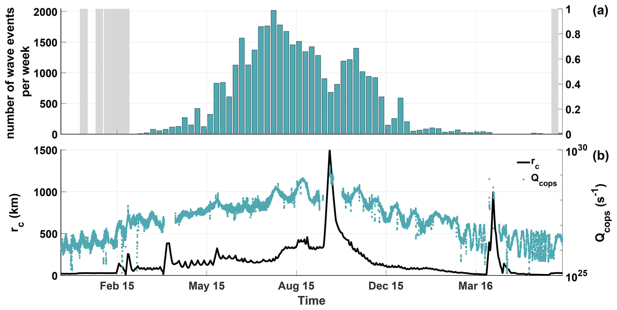
Figure 2Panel (a) depicts the number of observed steepened waves per week over the course of the mission. The gray areas mark the periods in which no magnetic field measurements were available. In (b) the water outgassing rate (Q) and the cometocentric distance (rc) are shown. The outgassing rate was computed using the Haser model (Haser, 1957) and local ROSINA-COPS measurements. A constant neutral gas velocity of 800 m s−1 was assumed. The neutral gas density measurements are noncontinuous, with occasional data gaps.
Shortly after the comet rendezvous on 6 August 2014, low-frequency, large-amplitude waves were found to dominate the magnetic field observations (Richter et al., 2015). Over the progression of the Rosetta mission, these singing comet waves (Richter et al., 2015, 2016; Heinisch et al., 2017; Goetz et al., 2020) slowly give way to a more turbulent interaction region with increasing outgassing rate. During these early months, only a few (<40) isolated instances of steepened waves were observed. Since the detection method was evaluated for different cometary activity levels, we can exclude that the low number of identified steepened waves is due to a bias in the detection method (Ostaszewski et al., 2020). The period from February to April 2015 marks a transition region in which the singing comet signature is not detectable anymore, and first occurrences of cavity crossings (Goetz et al., 2016a) and steepened waves were observed, which become increasingly prevalent as cometary activity increased. It is still uncertain if the singing comet waves cease to exist or if they are obscured by the increasingly turbulent field closer to perihelion. The exact nature of this transition region and the processes governing it require a more in-depth analysis, which is outside of the scope of this paper. Around the time of May 2015, a sudden steep increase in the number of observations above 500 per week is visible. In the month before and after, an average of 100 steepened waves per week is detected, with occasional peaks up to 400. From May until December 2015, the number of steepened waves, in general, follows the mean outgassing rate, where a high activity is associated with a large number of observed waves. Especially on the inbound leg toward the Sun, one can observe how the number of steepened waves steadily increases until it reaches a maximum at the beginning of August 2015, shortly before perihelion. Even though the water production rate further increases after perihelion passage, the number of observations starts to decline afterward. Simultaneously with the observed decline, the cometocentric distance increases. This behavior is particularly evident during the dayside excursion in September–October 2015 (Edberg et al., 2016). For this time interval, a significant decrease of observed steepened waves is visible, while the cometary water outgassing rate further increases. During the dayside excursion, the number of observations declines by half compared to adjacent time intervals. After reaching the furthest distance of 1500 km, Rosetta starts to approach the nucleus again, reaching a distance of 150 km in December 2015. During this time, the number of observations increased from around 800 to above 2000 per week, even though the water outgassing rate decreased from approximately 1029 to approximately 2×1028 s−1. During the excursion to the nightside of the comet in March 2016, the number of observed steepened waves was already too low to validate the observed distance dependency during the dayside excursion. It is worth noting that while a general trend in the number of observations is evident, the variations from week to week are still quite large. On occasion, the number of observations can even double compared to neighboring time intervals, while no corresponding signatures are visible, neither in the cometocentric distance, nor in the outgassing rate. However, the Haser model (Haser, 1957) assumes a spherically symmetric coma and therefore neglects variations due to zones of varying activity on the nucleus (Lai et al., 2019).
Since mass loading is one of the fundamental processes governing the solar wind–comet interaction, it may be a better measure for the steepened wave occurrence rate and can also give indications about the source of these waves. The local mass loading depends on the cometary activity as well as on the cometocentric distance (Biermann et al., 1967; Behar et al., 2016; Nilsson et al., 2017; Glassmeier, 2017). The strength of the local mass loading at Rosetta is given by the source term
where mi is the ion mass, νio the ionization frequency and nn the neutral gas density measured by ROSINA-COPS. Since we use the locally measured neutral gas density, variations due to cometary rotation and asymmetric outgassing are taken into account (Hansen et al., 2016; Lai et al., 2019). At 67P/CG, the dominant ionization processes are photoionization, electron impact ionization and charge exchange. The importance of the individual processes changes with heliocentric distance and location in the interaction region. For a strongly active comet and close to the nucleus (rc<1000 km), the dominant process is photoionization (Wedlund et al., 2017, 2019). The latter varies with distance to the Sun and is given by
where s−1 (Hansen et al., 2007) is the photoionization frequency at 1 au, and rh is the heliocentric distance in au. Engelhardt et al. (2018) showed that the number of observed density enhancements increases closer to the electron exobase, which is the boundary region between collisional and collisionless electrons. A similar dependence was reported for the number of diamagnetic cavity crossings by Henri et al. (2017). The electron exobase distance can be estimated from in situ neutral density estimates nn as
where rc is the cometocentric distance, and σen is the electron-neutral cross section. Following Henri et al. (2017) and Engelhardt et al. (2018), we assume cm2 for an averaged electron energy of ∼ 5 eV. Figure 3 shows the number of observed steepened waves per hour as a function of the mass source term (Fig. 3a) and the cometocentric distance expressed in terms of the electron exobase distance 3b. The rates were obtained by dividing the total number of steepened waves observed for a certain mass loading by the number of hours RPC-MAG operated during the respective local mass-loading conditions. The number of observed steepened waves increases linearly with the mass-loading strength up to a certain point, after which the detection rate stagnates at around 11 steepened waves per hour. As noted by Bieler et al. (2015), the gas production rate at 67P/CG is dominated by H2O, CO2 and CO. While the period considered in this study is heavily water-dominated (Läuter et al., 2020), CO2 and CO have a higher molecular mass. Hence, the observed stagnation may be caused by underestimating the local mass loading. Another possibility is that the observed plateau in the occurrence rate is caused by a saturation of the waves' generation mechanism. Ultimately, a more detailed investigation is needed to resolve this question. The increase of wave occurrences closer to the electron exobase is consistent with observations made by Engelhardt et al. (2018).
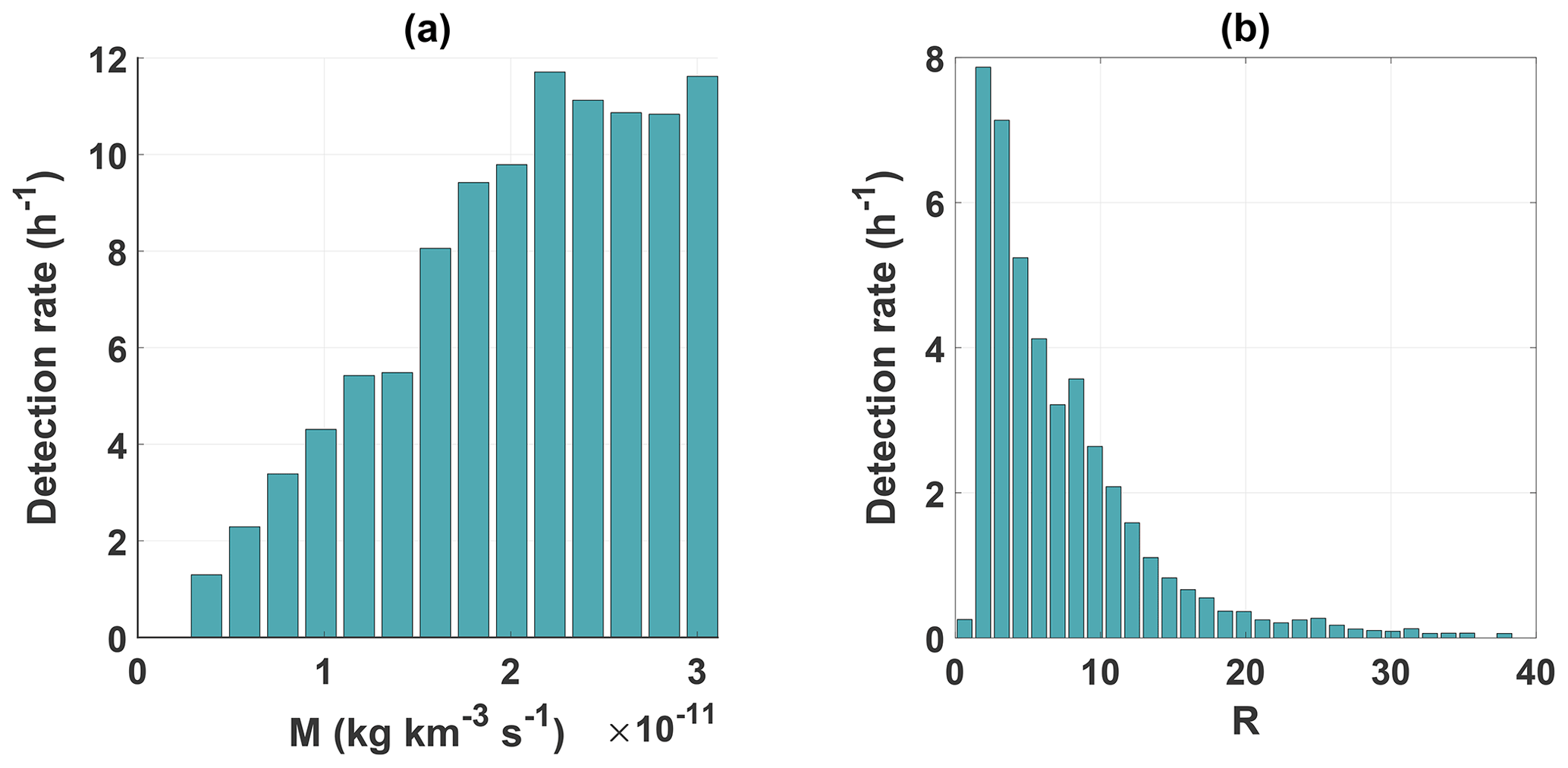
Figure 3Number of observed steepened waves per hour as a function of mass loading (a) and the normalized cometocentric distance R (b).
In general, the variations in the number of observations can be sufficiently explained by changes in the neutral outgassing rate and cometocentric distance (Figs. 2 and 3). However, in some instances, the number of observed steepened waves abruptly declines over the course of hours without any noticeable variations in either the neutral gas density or the cometocentric distance. Figure 4 shows the time between two steepened wave observations between May and September 2015. The time between observations is extremely variable, with values between 4 and 78 min. Striking are the occasional sharp increases in the time between observations; e.g., on 30 August 2015, the time increased from around 7 to 55 min within 1 d. For these intervals, the decrease in detected steepened waves was manually verified to exclude a bias in the automated detection procedure. Goetz et al. (2017) and Timar et al. (2019) noted that apart from the neutral gas density, solar wind conditions have a significant influence on the magnetic field at the comet. The dashed line in Fig. 4 shows the solar wind dynamic pressure extrapolated to Rosetta's location with the Tao model (Tao et al., 2005).
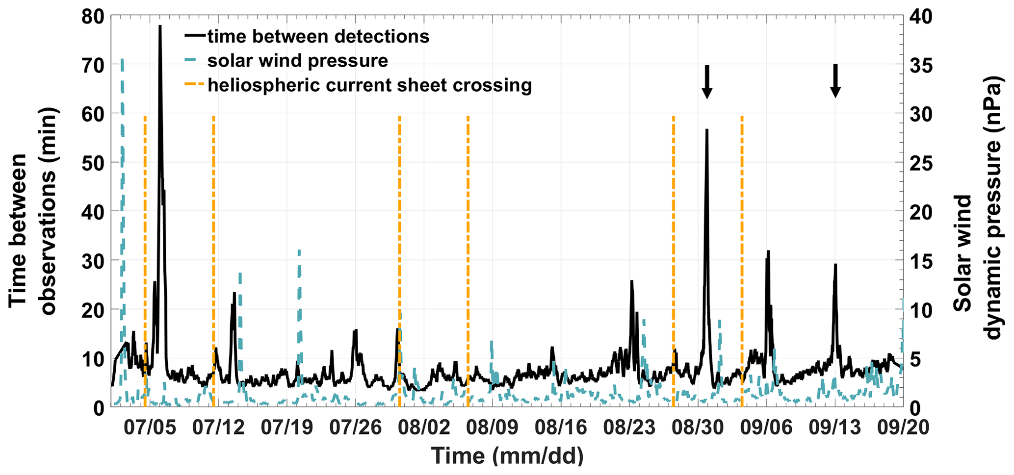
Figure 4Averaged time between detections (solid line) and the solar wind dynamic pressure (dashed line) from 1 July until 20 September 2015. The solar wind pressure was extrapolated from near Earth to 67P/CG using the model by Tao et al. (2005). The vertical lines denote the dates of HCS crossings. Occasional sharp increases in the time between detections are visible. Examples of the magnetic field magnitude for the occurrences marked by the arrows are shown in Fig. 5.
In some cases, these sharp increases in the inter-wave time coincide with increases in the solar wind dynamic pressure. However, most of the time, no correlation between the pressure and time between observations is visible. For the two particular cases marked by arrows, the magnetic field magnitude over a 1 h interval is illustrated in Fig. 5. On 14 September 2015, the magnetic field is dominated by long-period large-amplitude steepened waves. A day before, on 13 September 2015, the interaction region is completely different. Fluctuations occur on significantly shorter timescales with smaller amplitude, and the mean magnetic field strength increased from ∼ 20 to ∼ 40 nT. The direction of the mean magnetic field stays approximately constant, with on 14 September 2015 and on 13 September 2015. A similar situation can be observed for 29 and 30 August 2015. The previously observed long-period large-amplitude steepened waves are replaced by small-scale fluctuations, the mean magnetic field increases from ∼ 26 to ∼ 55 nT and the mean field direction only changes marginally from = (−0.04, 0.97, −0.23) to = (−0.13, 0.94, 0.32). The transition between regions occurs smoothly over a time span of dozens of hours, as indicated by the smooth increase in the temporal distance between observations (Fig. 4). No sharp changes in the magnetic field, which would indicate a crossing of some boundary, are observed during these time intervals. As Rosetta's position in the interaction region is approximately constant over a time span of 1 d, the characteristic increase in mean magnetic field strength is presumably caused by changing solar wind conditions. It hints at a compression of the interaction region, similar to the effects of a interplanetary coronal mass ejection (CME) impact (Edberg et al., 2016; Goetz et al., 2019).
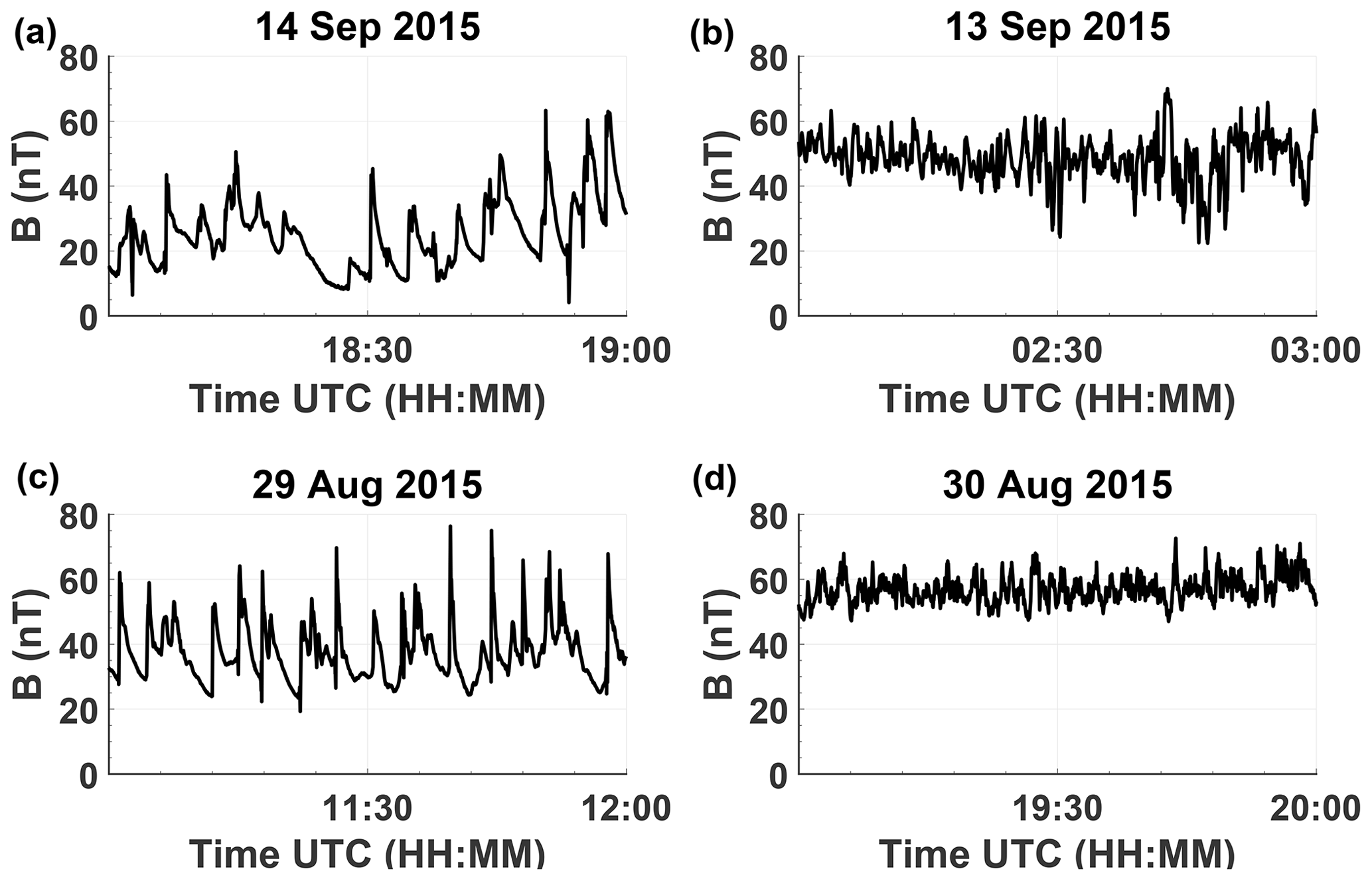
Figure 5In (a) and (c), typical examples of an interaction region dominated by large-amplitude steepened waves are shown. In (b) and (d), the interaction region 1 d later or earlier is shown. Instead of large-amplitude steepened waves, oscillations on smaller scales and with significantly smaller amplitude are visible, which resemble 1P/Halley's interaction region (Glassmeier et al., 1997). The illustrated time intervals correspond to the highlighted peaks in detection time in Fig. 4.
During the occurrence of these two examples, no apparent changes in the neutral gas density, spacecraft position or solar wind dynamic density, which could explain this complete change of nature of the interaction region, are visible. However, one has to keep in mind that the solar wind observations are not in situ measurements but rather measurements obtained near Earth and extrapolated to Rosetta's location with the Tao model (Tao et al., 2005) and may therefore be inaccurate. Another possible explanation are transient solar wind events. Candidates are CMEs, co-rotating interaction regions (CIRs) and heliospheric current sheet (HCS) crossings (Smith et al., 1978). Both CMEs (Edberg et al., 2016; Goetz et al., 2019) and CIRs (Hajra et al., 2018a) are known to compress the cometary interaction region and cause such increases in the magnetic field. Since HCS crossings are a reversal of the interplanetary magnetic field, it is unclear if they could affect the cometary interaction region in a significant way. However, adjacent to HCSs are very high plasma densities, which are likely able to compress the cometary interaction region in a similar way to CMEs and CIRs (Tsurutani et al., 2016). For the considered time intervals, no CME or CIR events were observed. As a reference, the Rosetta science event list was used (Rosetta Team, 2020). A list of HCS crossings is given by the Wilcox Solar Observatory (Svalgaard and Wilcox, 1976; Svalgaard, 2020). The dates of crossings are marked by orange vertical lines in Fig. 4. A direct correlation between HCS crossings and increases in time between observations is not visible. However, in most cases, an increase in the time between two detected steepened waves occurs within days after a HCS crossing. Overall, to determine the governing processes for these changes in the interaction region, a more in-depth analysis of the local solar wind conditions using different models and databases is necessary. For example, Rosetta-SREM (Standard Radiation Environment Monitor) measurements could provide additional information regarding solar wind conditions, and ENLIL simulations (Witasse et al., 2017) could be used to determine if transient solar wind events reach the comet at certain times. Since this is outside of the scope of this paper, it is left for further research.
Based on the shape of the magnetic field signatures, two types of steepened waves can be identified. In Fig. 6a, the prototypical steepened wave is displayed. It is characterized by a sharp increase in magnetic field magnitude on timescales of seconds to minutes, followed by a more gradual decline. The steep leading edge is typically observed first. The second type of steepened wave principally resembles the first, with the addition of oscillations at the leading edge. These types of dispersive effects are evident to varying degrees. In a weakly pronounced case, the dispersive effects cause an undershoot, which can vary between several nanoteslas (nT) up to tens of nanoteslas, at the foot of the leading edge. In a more developed state, multiple oscillations at the leading edge are present, for which frequency and amplitude visibly decrease with distance from the edge. These dispersive effects resemble the whistler packets observed at 21P/Giacobini–Zinner (Tsurutani et al., 1987) and in the Earth's foreshock (Hada et al., 1987; Greenstadt et al., 1995). It is worth noting that while the degree of dispersive effects differs significantly, the overall shape of the magnetic field signature is still remarkably alike. Steepened waves with dispersive effects constitute around 40 % of all observations. Of these, weakly pronounced effects are most frequent, whereas strong effects similar to Fig. 6b are comparably rare. Compared to observations at 21P/Giacobini–Zinner, where the high-frequency whistler packets accompanied the nonlinear wave, this percentage is remarkably low. Instances in which the oscillations are visible behind the steep edge can also be observed occasionally. Similar signatures have also been observed at 21P/Giacobini–Zinner, where magnetosonic waves developed a double peak in magnitude over time (Tsurutani et al., 1997; Szegö et al., 2000). Tsurutani et al. (1997) and Szegö et al. (2000) interpret the observations as the onset of a decay instability. Using simulations, Omidi and Winske (1990) were able to produce similar wave splitting features. Such wave splitting has also recently been observed for Alfvén waves (Tsurutani et al., 2018).
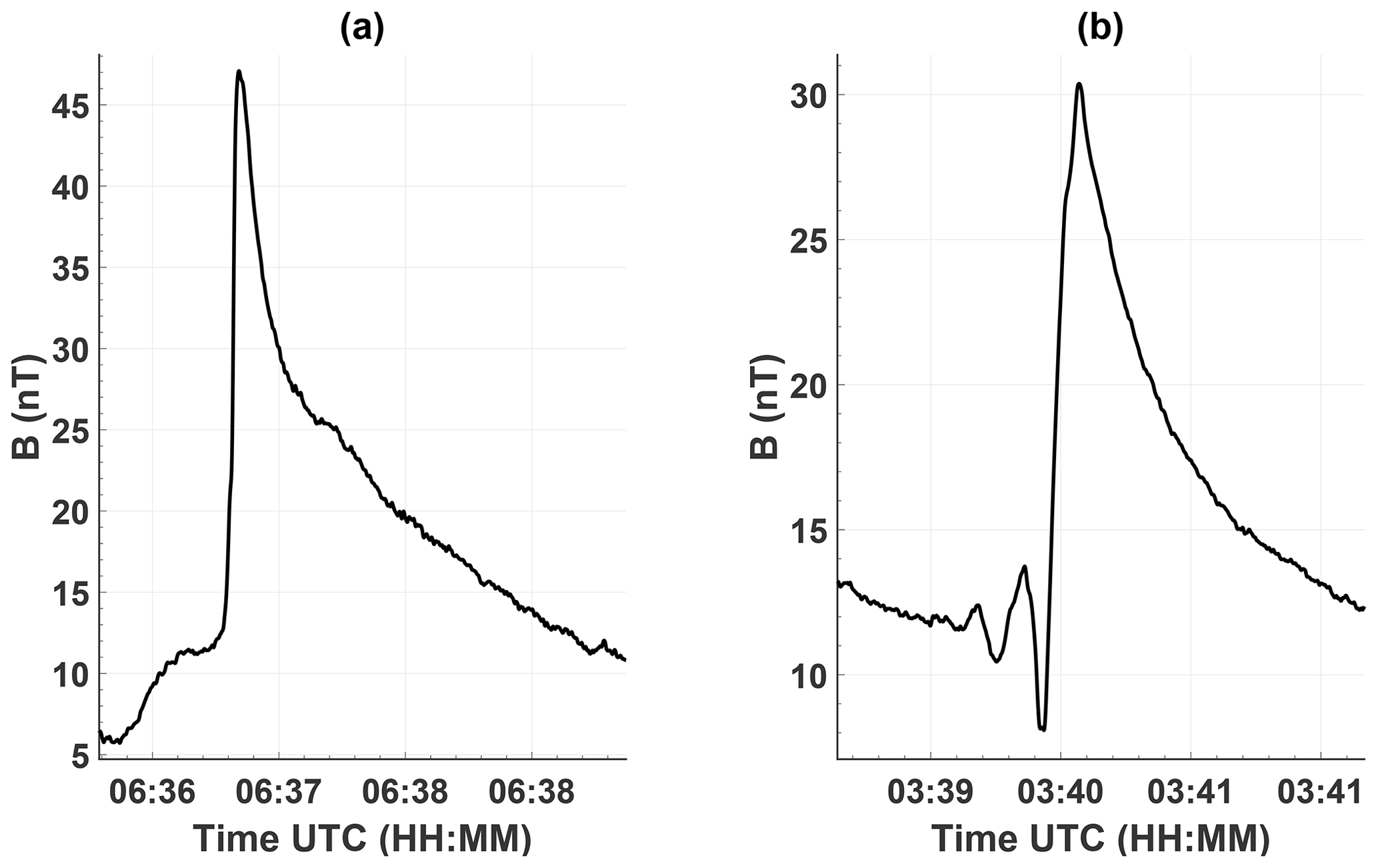
Figure 6Example of a typical steepened wave without dispersive effects on 20 November 2015 (a) and with dispersive effects on 3 August 2015 (b).
As is evident from Fig. 1, the amplitude, width and asymmetry of the steepened waves vary significantly. In order to derive these quantities in a consistent manner, a skew normal distribution (SND; Eqs. 4–6), as given by Azzalini (1985), is fitted to the magnetic field magnitude in intervals of interest. The SND was chosen because it is similar in shape to the steepened waves and provides comprehensive definitions of amplitude, skewness and width. Moreover, using a fit instead of directly computing amplitude and skewness from the magnetic field measurements, the coefficients of determination provide information on how well a candidate event resembles a typical steepened wave.
Usually, the skew normal distribution is described by three parameters, the location , the scale δ and the shape α. In this case, two additional parameters B0 and Bamp, that account for a background magnetic field and scaling to actual field strength respectively, are added:
To illustrate the validity of the approach we first compute an average shape of the magnetic field signature using a superposed epoch analysis (Chree, 1913, SEA) and then fit a skew normal distribution to the average shape using the Levenberg–Marquardt algorithm (Marquardt, 1963). For the averaging process, we used unfiltered data to ensure that the asymmetric shape, in particular the steep edge, of the wave is not affected. As amplitude and width of steepened waves vary widely, the amplitude was normalized and the intervals of interest resampled to the most common wave duration of 35 s. Moreover, we subtracted the mean magnetic field magnitude to account for varying offsets. Normalization of the magnitude is essential since otherwise the average shape will be skewed towards waves with a large amplitude. The signals are then temporally aligned by computing the shift using cross-correlation. Figure 7a shows the average shape of waves obtained by the SEA. As can be seen, the SND can capture the general characteristics of the waves adequately, with an adjusted R2 value of 0.98.
For the following analysis, the individual steepened waves are fitted, and only fits with an adjusted R2 value above 0.7 are analyzed further. Steepened waves with skewness values below 0.6 were discarded because they are not sufficiently asymmetric to be considered steepened. This reduces the number of steepened waves from initially approximately 70 000 to approximately 45 000.
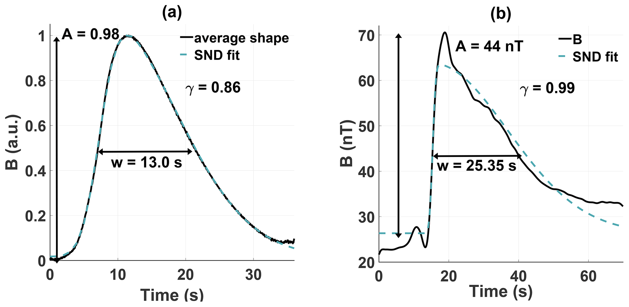
Figure 7Skew normal distribution fitted to the average shape (a) and an exemplary wave (b). Through the skew normal distribution, comprehensive definitions of amplitude, skewness and width are obtained.
The skewness γ and amplitude A of the wave are obtained by
where (Azzalini, 1985). Values for the skewness range from −1 for left-skewed distributions to 1 for right-skewed, where a value of 0 signals a symmetric distribution. As a measure of the width, the full width at half maximum (FWHM) is chosen, as it provides a well-defined point at which the widths can be compared. While the average shape is described well by the SND, individual waves can differ slightly in shape compared to the SND. In some cases, this can lead to errors in the determination of the amplitude, as shown in Fig. 7b. Hence, the amplitude is computed as the difference between the magnetic field signatures maximum and the footpoint in the magnetic field data.
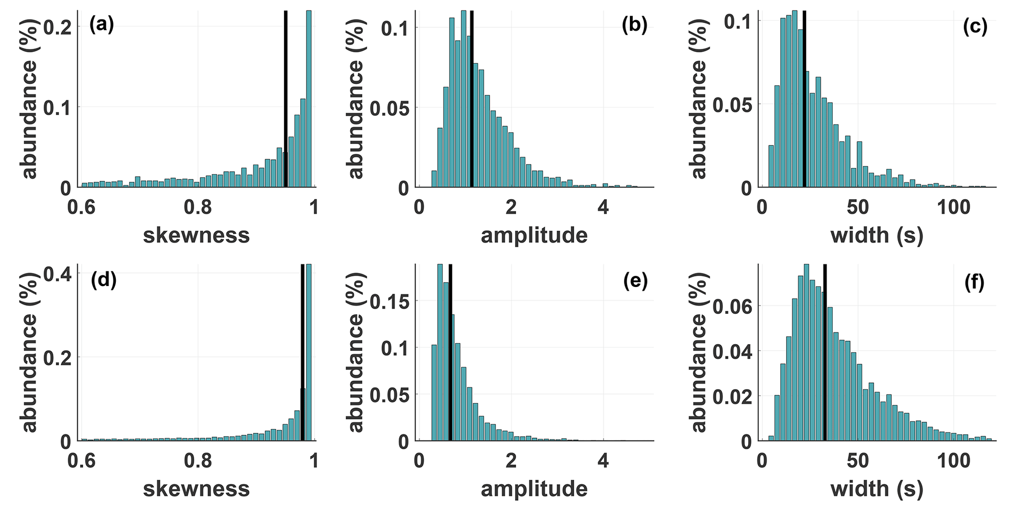
Figure 8Distributions of skewness, amplitude and width for different levels of cometary activity. Panels (a)–(c) show the properties of steepened waves for low to intermediate activity from 1 March to 1 June 2015 ( s−1). For a strongly active comet from 15 August to 15 September 2015 ( s−1), the properties are shown in (d)–(f). The abundance is normalized to the total number of observations in the respective interval. The black line marks the median of the respective distribution.
Figure 8 shows the distributions of amplitude, skewness and width for two different levels of activity. The amplitude was normalized to the magnetic field strength at the footpoint of the wave. The black line marks the median of the respective distribution. Panel (a) to panel (c) depict the distribution from 1 March until 1 June 2015, which corresponds to an intermediately active comet. In panel (d) to panel (f), the distribution moments for the duration of 1 month from 15 August until 15 September 2015, for a highly active comet, are shown. Independent of the activity level, waves with low and high skewness values can always be observed, with a general trend towards higher values. With rising activity, the distribution leans more towards higher skewness values, which can be quantified by the median of the distribution. In Fig. 8, it can be seen that the median rises from 0.93 to 0.98, showing that the number of waves with high skewness increases with cometary activity. The distribution of amplitudes ranges from values around 0.3 to around 4, which shows that the waves can be highly nonlinear. However, in contrast to the median of the skewness, which increased with activity, the amplitude median decreases from 1.2 to 0.8. The absolute amplitude median, on the other hand, increases slightly from 18 to 22 nT. Lastly, more waves with larger width can be observed at higher activity. Note that the width can only be measured in time since information about the propagation velocity is not available. Therefore, differences in width are only partially features of the waves; changes in the bulk velocity of the propagation medium can also cause these variations.
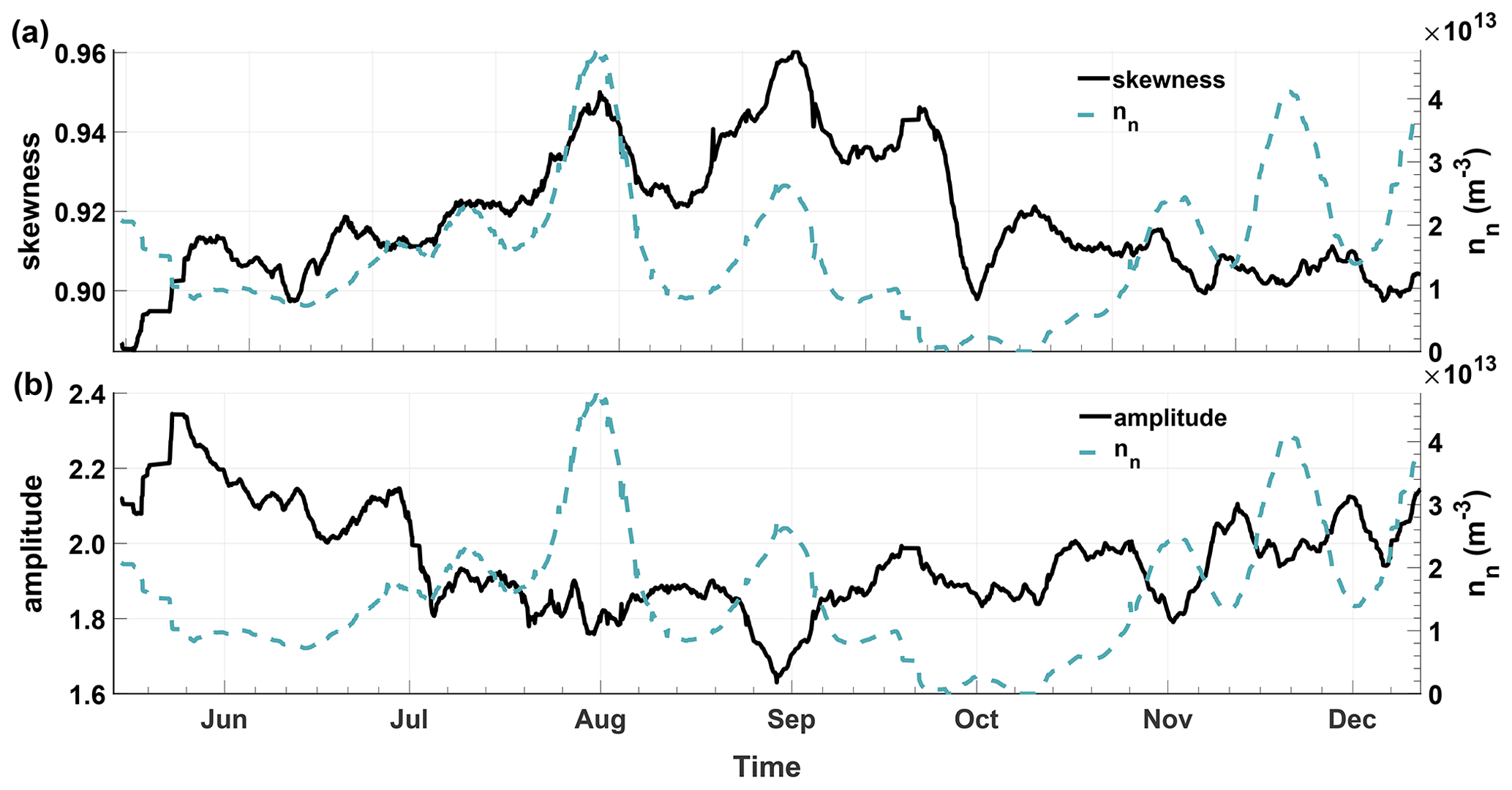
Figure 9Averaged skewness and neutral gas density from 14 May to 12 December 2015 (a). In (b) the averaged amplitude and neutral gas density are shown. While the skewness exhibits a clear correlation with the neutral gas density, especially until October, the amplitude is mostly anti-correlated to the neutral gas density.
Figures 3 and 8 illustrate that the properties of the waves are governed by variations in the local plasma environment. Hence, the local plasma density and neutral gas density are expected to influence the development of the waves. In Fig. 9a, the skewness and neutral gas density, averaged over 1 week, are shown as a function of time. Until late September 2015, the skewness and neutral gas density are in good agreement, with a correlation coefficient of ρ=0.76. In contrast, the amplitude shows an apparent anti-correlation with , which is especially evident around September.
The minimum variance analysis (MVA) by Sonnerup and Cahill (1967) and Sonnerup and Scheible (1998) is a method frequently used to determine the normal of a boundary or the wave propagation direction. To determine the minimum variance direction of the steepened waves, in a first step, a sixth-order Butterworth lowpass filter (Butterworth, 1930) with a cutoff at 500 mHz was applied to the magnetic field observations to exclude high-frequency oscillations. The cutoff frequency was chosen such that the steep leading edge was unaffected by the filter. In order to exclude steepened waves which do not exhibit a distinct pattern, only results with a corresponding eigenvalue ration of are selected. On average, the waves have a mean eigenvalue ratio of 13.7.
As a reference point, the angle between minimum variance direction and the local cometary background field is calculated. For such a turbulent interaction region as the inner coma, it is difficult to define what constitutes a background field. Following Goetz et al. (2017), the background field is assumed to be the mean magnetic field, which was obtained by applying a sixth-order Butterworth lowpass filter with a cutoff frequency of 0.1 mHz, followed by averaging over a sliding window with a size of 20 min and a displacement of 10 min to the magnetic field components. For the cutoff frequency, a value was chosen so that all local disturbances, especially the steepened waves, which are very broad in the frequency space, were removed, while global variations caused by, e.g., diurnal changes remained visible. As the directions of minimum variance, as well as the cometary background field, are susceptible to offsets in the components, the following analysis was only performed for the periods in which observations of diamagnetic cavities were available to adjust the offsets. Therefore, time frames before 20 April 2015, during the dayside excursion and after 17 February 2016 are excluded.
The angle Φ(a,b) between two vectors a and b can be calculated following
Because of the ambiguity of the MVA to the sign, the range of values for the angle Φ spans over [0, 180∘]. As mentioned by, among others, Narita (2017), the minimum variance analysis fails for linearly polarized waves because the polarization plane is not uniquely determined. Therefore, all waves with an ellipticity above 0.9 are disregarded for the analysis of the minimum variance direction. In general, the steepened waves are highly elliptically polarized, with a mean ellipticity of 0.7. As a consequence of this approach, the number of valid events is significantly reduced to around 15 000.
The histogram in Fig. 10a shows the abundance of angles between the minimum variance direction of the waves and the cometary background field.
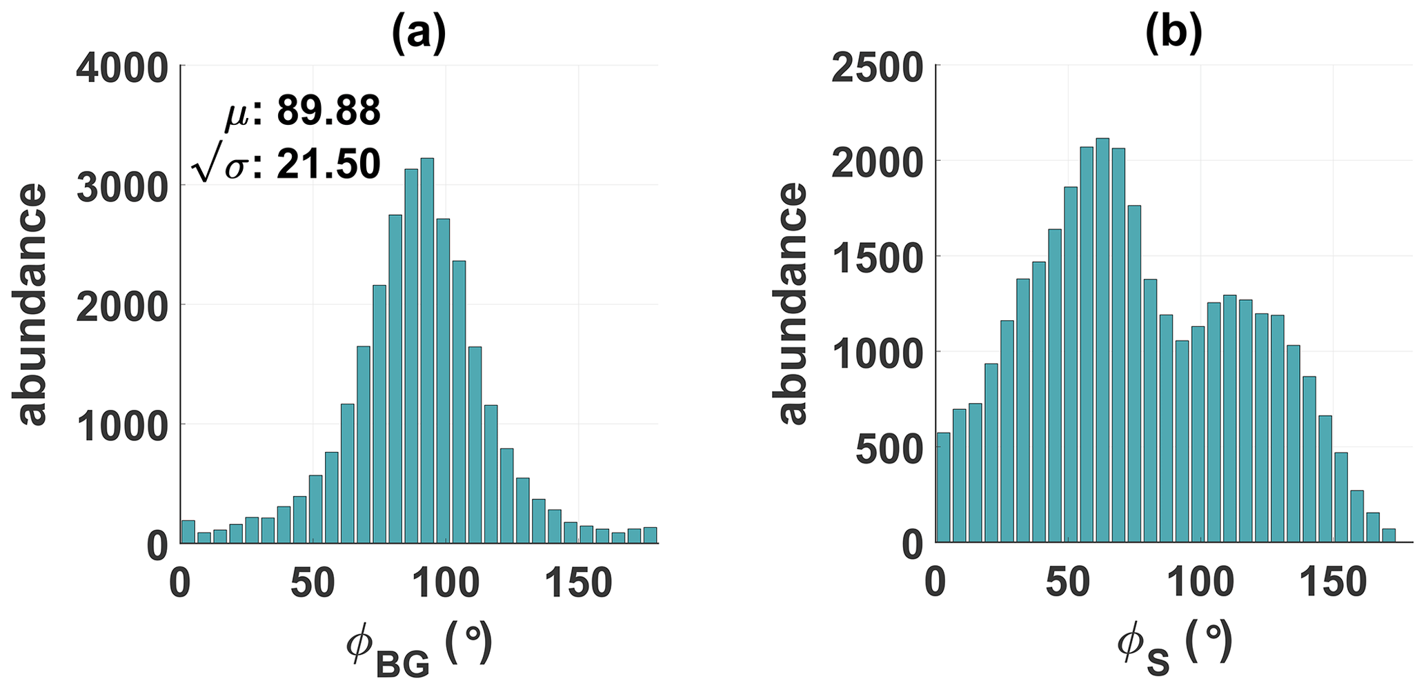
Figure 10Histograms of the angle between the minimum variance direction and the background magnetic field (a) and the spacecraft-Sun connection line (b). The waves propagate predominantly perpendicular to the background field and at an angle ±65∘ to the Sun.
Due to the larger circumference on a sphere for Φ≈90∘ than for Φ≈0∘, the number of observed angles will be biased towards 90∘. To remove this bias, the number of observations Ni for bin i were multiplied by sin (ϕi), where ϕi is the corresponding angle for bin i. As can be seen, the minimum variance direction follows a remarkably well-defined normal distribution, with a mean of μ=89.88∘ and a standard deviation of ∘. Thus, the waves propagate predominantly perpendicular to the cometary background field. However, as Eq. (9) defines an angle in 3D space, it is invariant to rotation along the background magnetic field direction. Therefore, the direction of the minimum variance in the plane perpendicular to the background field vector is uncertain by 180∘. As a second point of reference, the angle between the minimum variance direction and the Sun is shown in Fig. 10b. The distribution has a bimodal shape, with maxima around 65 and 115 or ±65∘ due to the MVA ambiguity. This does not contradict the fact that the waves propagate perpendicular to the background magnetic field, since for a strongly outgassing comet, the magnetic field drapes around the comet (Goetz et al., 2017; Volwerk et al., 2018). Consequently, the background magnetic field is predominantly oriented in the x direction sun- or antisunwards. The asymmetric shape may be introduced by orbital configuration and is therefore not necessarily of scientific interest. Figure 11 shows Rosetta's trajectory from 5 June to 15 August 2015, and the propagation direction of the waves is indicated by black arrows.
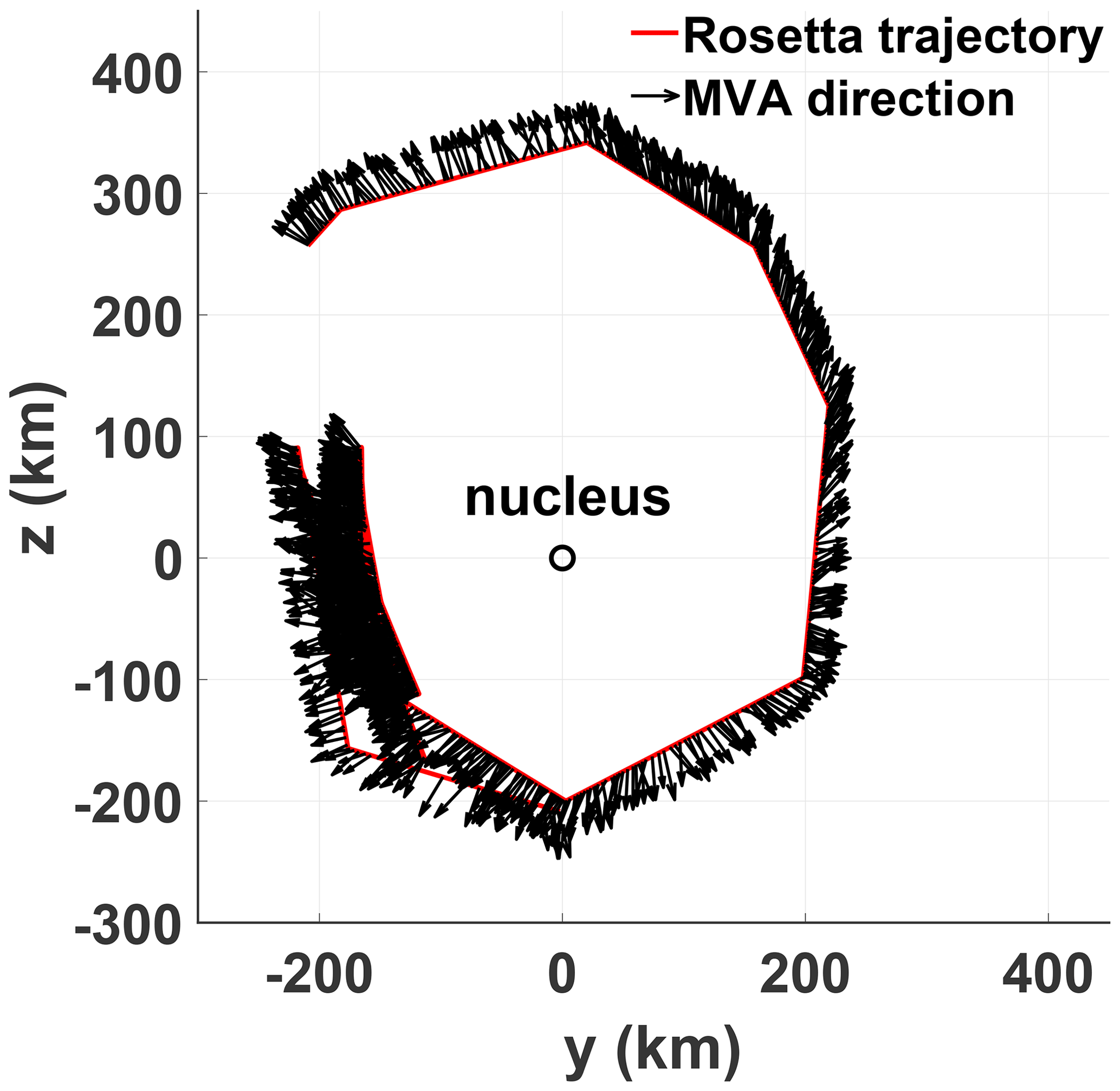
Figure 11Illustration of the minimum variance angle projected onto the yz plane of the CSEQ frame for the time interval from 5 June to 15 August 2015. The solid red line at the base of the black arrows denotes the spacecraft trajectory, while the black arrows show the waves' minimum variance direction. The vectors were adjusted so that all have the same orientation, which was arbitrarily chosen to be pointing away from the nucleus.
During this time interval, Rosetta was mainly in a terminator orbit, with minimal variation in the x direction. In the figure Rosetta's trajectory and the minimum variance direction of the waves are projected onto the yz plane of the CSEQ coordinate system. The minimum variance direction was adjusted so that every instance has the same orientation, which is arbitrarily chosen to be oriented away from the nucleus. A moving average for a time interval of 2 h is then applied to the minimum variance direction. To further increase the visibility, only every 10th vector is plotted. It is clearly visible how the waves change their propagation direction over the course of Rosetta's trajectory, so that, in Fig. 11, they are oriented approximately away from the comet. The pattern that the minimum variance direction exhibits in Fig. 11 resembles the general motion of cometary ions (<60 eV) close to the nucleus (Odelstad et al., 2018; Nilsson et al., 2020). A similar flow pattern was also found for accelerated ions (40–80 eV) inside and outside of the diamagnetic cavity (Masunaga et al., 2019). In both cases, a significant antisunward motion of the ions toward the tail was reported. Due to the ambiguity of the MVA, it is unclear if the waves have a sun- or antisunward motion. In the configuration chosen in Fig. 11, the waves exhibit a slight sunward motion.
The main properties of these steepened waves can be summarized as follows:
-
The number of observed steepened waves predominantly depends on the mass loading. A similar dependence was also found for the distance to the electron exobase, where more steepened waves were observed closer to the exobase. Influences of extreme solar wind conditions may be seen in occasional sudden increases of the time between observation of two steepened waves.
-
Steepened waves can be grouped into two categories, those with dispersive effects and those without. In the former case, high-frequency oscillations are visible at the leading edge of the steepened wave.
-
Skewness and amplitude of the steepened waves depend on the neutral gas density, where the former increases with density, and the latter decreases.
-
Based on an MVA, these waves propagate perpendicular to the background magnetic field and at an angle of ±65∘ to the Sun–comet line. The minimum variance direction of these waves resembles the flow pattern of cometary ions close to the nucleus. Propagation perpendicular to the background magnetic field is typical for fast magnetosonic waves.
The compressional nature of these waves (Engelhardt et al., 2018; Hajra et al., 2018b) and the mainly strongly oblique propagation direction are indicators that they behave like fast magnetosonic waves. Hence, assuming an initial wave-like disturbance in the plasma and magnetic field, we investigate in the following section if the observed asymmetric plasma and magnetic field enhancements can be described as nonlinear phase-steepened waves in a consistent manner using a modified 1D MHD model.
Since the observed nonlinear waves predominantly propagate perpendicular to the background magnetic field, the 1D assumption is justified. As the inner coma is characterized by a high neutral gas density in comparison to the plasma density, and the wave processes are sufficiently slow, it is essential to take neutral gas effects into account as well. This leads to additional damping effects based on ion-neutral and electron-neutral collisions. In general, the damping rate is a function of the wave frequency and will therefore affect the skewness of the wave. Thus, we can obtain an estimate of the local effective wave damping rate using the observations of skewness and amplitude and by modeling the wave evolution using a modified 1D MHD model.
During the high activity phase, the plasma in the innermost interaction region is predominantly of cometary origin. The ion composition close to the nucleus changes with heliocentric and cometocentric distance. However, the three dominant species H3O+, NH and H2O+ all have a mass-to-charge ratio of 18–19 (Heritier et al., 2017). Hence, we model the charged plasma component using a single fluid, with a mass-to-charge ratio of 19 . The behavior and damping rates of waves in a partially ionized plasma are heavily influenced by the complex interaction between ions and neutrals (Zaqarashvili et al., 2011; Soler et al., 2013; Vranjes, 2014; Martínez-Gómez et al., 2018). Among the main dissipation mechanisms are resistive dissipation, viscous dissipation and ion-neutral friction. These mechanisms depend on the properties of the ambient plasma, in particular on the ion-neutral or electron-neutral collision frequencies. To correctly model this behavior, a multi-fluid model describing the interaction between the charged and neutral fluid is necessary. However, due to temporarily and spatially limited plasma measurements (in particular ion velocities), the wave evolution, especially the ion-neutral interaction, cannot be sufficiently resolved. Hence, with only limited information available, such a high level of theoretical detail is impractical. Moreover, the dynamics of the neutral fluid beyond the ion-neutral and electron-neutral interaction is not of interest for this study. Thus, to reduce the complexity of the model, we parametrize the wave damping using an effective viscosity and resistivity. Then the additional dissipation induced by the ion-neutral and electron-neutral interaction can be approximated without going into too much detail about the underlying physical processes. We consider two different mechanisms, resistive and viscous damping, since they depend on different plasma parameters. By comparing the values obtained through simulations with suitable reference values, constituent processes influencing the wave damping can be identified. Assuming , and , the 1D fluid equations with resistive and viscous contributions are (Warburton and Karniadakis, 1999)
where the total energy density is given by
Herein, B′ is the magnetic field, u′ the plasma bulk velocity, ρ′ the mass density, p′ the pressure, the internal energy, η′ the resistivity and ν′ the kinematic viscosity. The prime denotes normalized quantities, where the mass density is normalized by the equilibrium mass density ρ0, the bulk velocity by the Alfvén speed vA, the magnetic field by B0, the time by the ion gyroperiod , space by the ion skin depth vA⋅Ωi, the resistivity η by and the kinematic viscosity ν by .
In this model, the wave propagates perpendicular to the background field. Therefore, only the fast mode is described. Moreover, the Hall term in the induction equation vanishes. Consequently, dispersive effects as seen in Fig. 6 are not modeled. However, this setup has the advantage that the numerical solution for the magnetic field is inherently divergence-free, so that no additional divergence cleaning steps have to be taken (Ranocha et al., 2020). Due to the nonlinear terms, an initial disturbance in the plasma will steepen and eventually resemble the waves observed at 67P/CG. At some point, the nonlinear steepening will be constrained by dissipative effects. Due to the frequency-dependent damping, the skewness of the steepened wave will also be affected. High-frequency wave packets as seen in Fig. 6 and at 21P/Giacobini–Zinner (Tsurutani et al., 1987) arise when dispersive effects outweigh dissipative ones and balance the nonlinear steepening.
Nonlinear hyperbolic systems are known to be able to develop shock solutions, which are difficult to treat numerically, especially for methods based on discretizing derivatives directly. Unsuitable numerical schemes may develop nonphysical solutions, e.g., in the form of spurious oscillations. Hence, Clawpack, a software suite specifically developed to solve nonlinear conservation laws, balance laws and other first-order hyperbolic partial differential equations, was used (Clawpack Development Team, 2019). To solve systems of nonlinear hyperbolic equations, Clawpack uses a high-resolution wave propagation algorithm (Ketcheson et al., 2013; LeVeque, 2002). The algorithm is based on a finite volume method utilizing Riemann problems to determine the update of the numerical solution. For this study, the Roe approximate Riemann solver (Roe, 1981) and spatial discretization of second-order are used. For time integration, a fourth-order strong-stability-preserving method (Ketcheson et al., 2013) is chosen, and at all boundaries of the simulation box, nonreflecting outflow conditions are enforced.
Since the steepened waves in Fig. 1 do not exhibit any apparent periodic behavior, an initial condition of the form of a single pulse
is chosen. Due to the factor 4ln (2) in the argument of the exponential function, w corresponds to the full width at half maximum. Following Shukla et al. (2004), the corresponding disturbances in ρ, u and p for a fast-mode-type wave are
with the integration constant
In the scope of this study, we do not explicitly model wave excitation but instead assume that the initial disturbance is present at t=0. Various plasma instabilities triggered by the interaction between the solar wind and newly implanted cometary ions (Wu and Davidson, 1972; Tsurutani, 1991; Gary, 1991; Motschmann and Glassmeier, 1993; Meier et al., 2016; Glassmeier, 2017) are known to excite large-amplitude low-frequency waves, which could be the initial disturbance from which such steepened waves develop. We also want to note that at 26P/Giacobini–Zinner (Tsurutani et al., 1990) and at 19P/Borrelly (Tsurutani et al., 2013), large-amplitude symmetric pulses, similar to the initial disturbance chosen for the simulation, were found near the bow shock region. Figure 12 shows the solution to Eqs. (10)–(13) computed with Clawpack in the domain for the initial condition given by Eqs. (15) to (18) with the amplitude A=2, width w=3, displacement δx=30, , plasma and grid size .
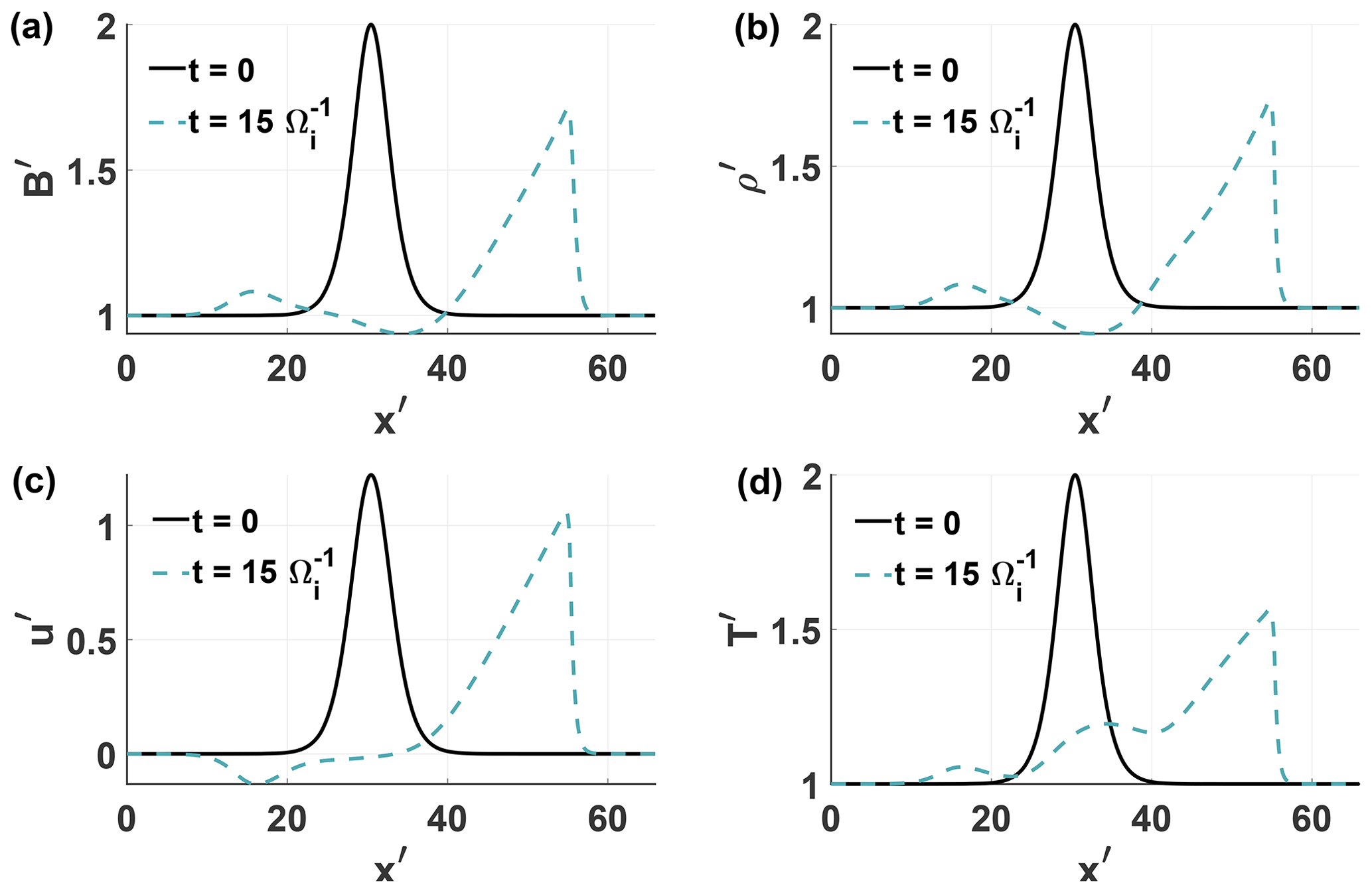
The solid black line denotes the initial condition for the magnetic field B, mass density ρ, velocity u and temperature T. The dashed line shows the solution after a time . The nonlinear steepening, as well as the decrease in amplitude, can be observed for all four quantities. A small part of the initial disturbance can be seen propagating to the left, which is evident in the negative velocity. To ensure that the dissipation is not numerical, simulations with identical initial conditions but increasing resolution were run. All simulations produced the same results, independent of the chosen grid size .
In Fig. 13a, the steepening time tst, which is defined as the time at which the skewness has reached its maximum value, as a function of the plasma β is shown. It decreases with an increasing plasma β. A similar dependency is observed for the amplitude of the initial disturbance in Fig. 13b. In general, tst declines when the phase velocity of the wave increases. Times in SI units can be obtained by multiplying tst by the ion gyration time . For typical values s rad−1, we obtain steepening times in the range between 30 to 460 s. With typical phase velocities around the order of km s−1, a wave travels between 300 and 4600 km before reaching its maximum skewness. In both cases, the cometary interaction region, with an estimated extent of ≈ 10 000 km, is larger than the distance traveled by the wave. Hence, fast-mode waves at 67P/CG have enough time as well as space to fully steepen in the interaction region. Furthermore, it can be assumed that deep in the interaction region, where Rosetta was mostly located, the waves will already have steepened to their maximum skewness. Then the observed skewness of the wave is a function of its amplitude, width and the local plasma properties, in particular the plasma β, the resistivity and the viscosity.
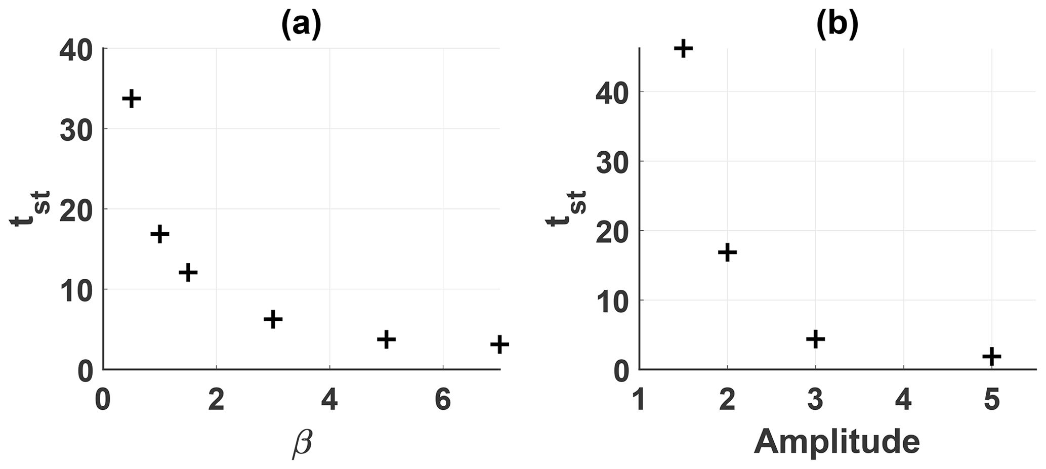
Figure 13Normalized steepening time as a function of the plasma β (a) and the amplitude (b).
To obtain an estimate for the effective plasma resistivity and viscosity, the relation between skewness, viscosity, resistivity and the plasma parameters needs to be modeled. In Fig. 14, the maximum skewness as a function of viscosity is shown for different amplitudes A (panel a), widths w (panel b) and plasma β (panel c). In general, the skewness depends on the ratio between the nonlinear and diffusive terms. Since diffusive terms tend to smooth large gradients, the skewness decreases with increasing viscosity. The strength of the nonlinear term directly depends on the amplitude of the disturbance. Thus, for higher amplitudes, the steepening is more effective than diffusion, and higher skewness values can be reached. The behavior for an increase in the width w is similar. The second spatial derivative predominantly dampens structures on small scales. Hence, the damping effect is weaker the larger the structure is. In comparison to the amplitude and width, the viscous term is virtually independent of β. Both the effectiveness of the nonlinear and the viscous term increase with the plasma β. As a consequence, the influence of both terms on the skewness is approximately balanced out.
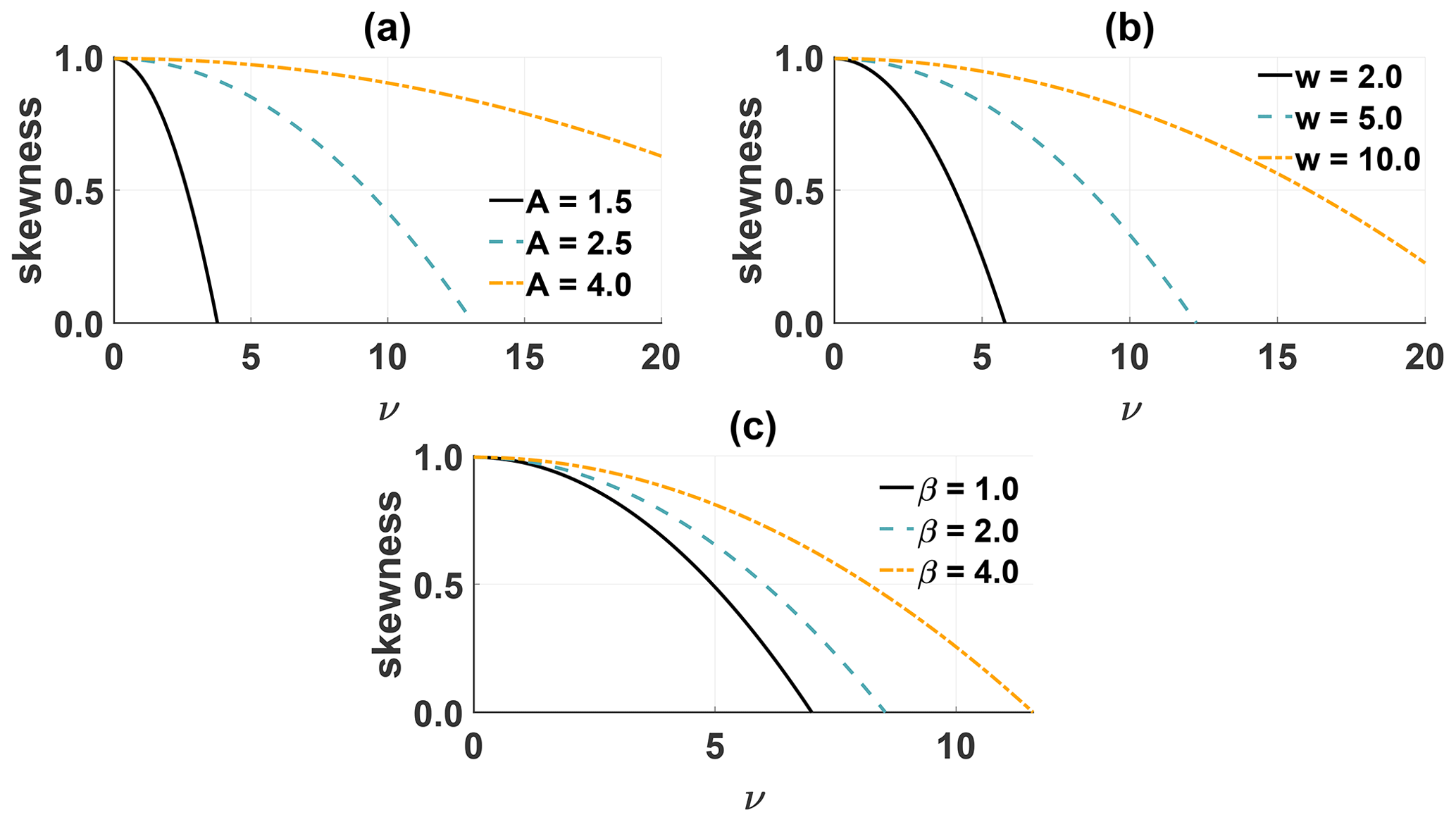
Figure 14Skewness as a function of the kinematic viscosity for different values for the amplitude (a), width (b) and plasma β (c).
Since the width w of the waves cannot be measured directly, an approximate value from the temporal width of the steepened waves and the local magnetosonic speed is used for the following simulations. Based on this approximation, the waves have a width of w=4, with a standard deviation of 2 in normalized units. As a consistency check, we computed the temporal width of the simulated waves at different times in the simulation and compared them with observed temporal widths of the waves (Fig. 8). Depending on the parameters for the initial condition and s rad−1, we obtained durations between 10 and up to 150 s, which is consistent with the observed durations. For fixed initial width, the approximation for the effective viscosity only depends on the skewness and amplitude of the wave. The dependency of the latter is that of a quadratic equation of the form
where c=0.955 is the maximum skewness value given by the SND, S(A,ν) is the skewness and
is a parameter depending on the amplitude. The coefficients , and p3=1.79 are obtained by fitting the value p(A) for different amplitudes. Solving for ν in Eq. (20) yields the inverse equation
from which an estimate of the effective viscosity can be obtained if the amplitude A and the skewness S are known. For the effective resistivity, additionally the dependency on β has to be modeled:
with the coefficients p1=0.282, p2=0.486, , , p5=1.117 and p6=0.366. Solving Eq. (24) for η yields
Over the course of a simulation, the amplitude A decreases, while the width w increases due to the presence of diffusive terms. Since it is uncertain where these waves are excited and how far they had traveled before Rosetta observed them, no information about the wave properties at the point of excitation is available. Hence, for lack of better information, the observed values for the amplitude and width are used in Eqs. (22) and (25).
As a quality measure, the computed values are subsequently compared to suitable reference values. For the dynamic viscosity, the definition from Khodachenko et al. (2004)
with , is chosen as a reference. The expression used for the viscosity is highly simplified. A more complex and detailed expression can be found in, e.g., Zhdanov (2002). However, for typical conditions at 67P/CG, we obtained similar values for Eq. (26) and the expressions given by Zhdanov (2002). Hence, in the following, the simpler expression Eq. (26) will be used. The resistivity is governed by electron-neutral collisions:
Since νen≫νei, the contribution through ion-electron collisions was neglected. The collision frequencies are given by
To facilitate a comparison between computed and reference values, Eqs. (26) and (27) have to be normalized in accordance with Eqs. (10) to (13):
Values for the electron temperature Te, the momentum transfer cross section σin and σen and the ion velocities vi have to be estimated, as no time-resolved measurements for longer periods are available. For the electron temperature, a mean value of Te=5 eV is assumed (Henri et al., 2017; Engelhardt et al., 2018; Hajra et al., 2018b). From Table 5 in Itikawa and Mason (2005), the corresponding momentum transfer cross section for electron collisions with H2O+ is obtained, i.e., m2. A mean value of vi=5 km s−1 for the bulk ion velocity is taken from Vigren et al. (2017) and Odelstad et al. (2018). Shortly after ionization, the cometary ions have approximately the same temperature as the neutral gas, i.e., Tn≈180 K. This was confirmed by Gunell et al. (2017), who studied ion acoustic waves at a weakly active comet 67P/CG (January 2015). However, Gunell et al. (2017) also reported on a heated ion population around kBTi≈1 eV. Such a warm ion population was also observed at 1P/Halley (Schwenn et al., 1988). Haerendel (1987) and Cravens (1987) argued that frictional heating between the ions and neutrals was responsible for the warm ion population. A similar process is also expected to heat ions at 67P/CG in the strongly active phase. Hence, for the following analysis, eV is assumed. For a solar wind primarily mass-loaded with H2O+ the ion-neutral momentum transfer cross section was estimated to be m2 (Mendis et al., 1986; Buti and Eviatar, 1989; Hajra et al., 2018b; Mandt et al., 2019). However, as stated by Mendis et al. (1986) and Gunell et al. (2017) the uncertainty of the cross section is significant, as no reliable laboratory measurements are available. Using the values given above, typical dynamic viscosities and resistivities are kg ms−1, Vm A−1 and in normalized units , . The difference between and amounts to a factor ∼ 1000. Hence, compared to the viscosity, the resistivity due to electron-neutral collisions is negligible. At high gas production rates, collisional cooling of electrons can reduce the electron temperature below 0.1 eV, which is more than an order of magnitude lower than the initially assumed 5 eV. For such low temperatures, the momentum transfer cross section is m2 (Itikawa and Mason, 2005). This yields a mean resistivity Vm A−1, which is slightly larger than the value for the warm electron population but still significantly smaller than the viscosity.
Figure 15 shows the distribution of , , ηsim and νsim. The reference values and were computed using Eqs. (31) and (30), and the viscosity νsim and resistivity ηsim approximations were computed using Eqs. (22) and (25). The shape of the distribution, similar to a Rayleigh distribution, can be reproduced for both cases.
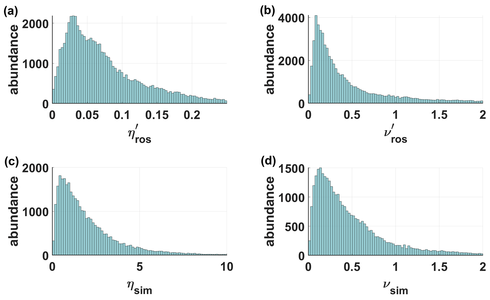

Figure 16Averaged computed kinematic viscosity νsim and reference kinematic viscosity over time for four different time intervals in 2015.
The resistivity approximation ηsim exceeds the reference value by a factor of 100. Investigating diffusion at Earth's magnetopause Nabert (2017) obtained an estimate for the plasma resistivity of Vm A−1. As a typical length scale of the system, Nabert (2017) assumed 700 km, which is comparable to the length scales of the steepened waves. The resistivity value given by Nabert (2017) fits the values obtained by our model quite well ( Vm A−1); however it is also multiple orders of magnitude higher than the Spitzer resistivity. Even for the high neutral gas densities in the inner coma, the resistivity governed by electron-neutral collisions is too low to explain the observed variation in the skewness. Hence, electron-neutral collisions likely do not influence the wave damping mechanism. On the other hand, the viscosity approximation νsim agrees well with the respective reference values . As a second reference, typical values for the dynamic viscosity in the Solar chromosphere, with values for ion temperature, density and neutral density given by Fontenla et al. (1993), lie in the range 10−9 to 10−7 kg ms−1 (Vranjes, 2014), which are comparable to the values at 67P/CG. Since the approximated diffusivities from the simulation agree well with the given reference values, the observed steepened waves can be, on average, described by a combination of nonlinear steepening and a diffusive process balancing said steepening. Dispersive effects as seen in Fig. 6b are secondary to diffusive effects, as the waves propagate predominantly perpendicular to the background field.
Figure 16 shows time-averaged values of νsim and for four different time intervals. Due to the dynamic nature of the interaction region, a comparison is only reasonable on long timescales. Hence, each illustrated interval is between 2 weeks and 1 month long. Moreover, a moving average with a window size of 2 d was applied, which encompasses four rotational periods of the comet. The model underestimates the viscosity slightly by a factor up to 2. However, the effective viscosity is able to reproduce variations over time, which is indicated by the high correlation coefficients (ρcorr>0.7). In contrast to the resistivity, the viscosity is predominantly influenced by the ion-neutral interaction. Since the variations in the approximated viscosity are sufficiently matched by the reference values, the damping mechanism is likely influenced by the ion-neutral interaction. However, we note that due to temporarily and spatially limited ion temperature and velocity estimations, the ion-neutral collisionality can only be roughly approximated.
We present a comprehensive statistical analysis of large-amplitude asymmetric waves in the inner coma of comet 67P/CG from December 2014 to June 2016. The around 70 000 identified steepened waves were analyzed to characterize these waves, in particular in relation to the evolution of the cometary interaction region and the changing plasma conditions in the inner coma of 67P/CG. We observe that the number of detected steepened waves depends on the local mass loading. A similar dependence was also found for the distance to the electron exobase. From May to December 2015, these waves dominate the innermost interaction region with typical times of 5–10 min between two observations. During this period, occasional intervals over 1–2 d, in which these waves vanish, were observed. This change of the interaction region is likely caused by transient solar wind events; however a more detailed study is needed to ultimately determine this. Based on a minimum variance analysis, the waves' propagation direction and ellipticity were determined. On average the waves are highly elliptically polarized, with a mean ellipticity of 0.7. The propagation direction is approximately perpendicular to the background magnetic field, which is typical for fast magnetosonic waves. The compressional nature of the waves is further supported by accompanying enhancements in the electron density (Engelhardt et al., 2018; Hajra et al., 2018b). The waves propagate approximately at an angle of ±35∘ to the spacecraft–comet line and at an angle of ±65∘ to the Sun–comet line. The pattern the minimum variance direction exhibits resembles the general ion motion close to the nucleus. Due to the ambiguity of the MVA to the orientation, it is unclear if these waves originate from the inner coma and propagate outwards or if they originate from outer regions and propagate inwards.
By fitting a skew normal distribution to the magnetic field magnitude, comprehensive measures for the amplitude, width and skewness of the waves were obtained. While the skewness increases with rising neutral gas density, the amplitude decreases, and the width shows no apparent correlation. Using a 1D MHD model, we showed that the waves can be described as nonlinear phase-steepened waves balanced by a combination of nonlinear steepening and dissipative effects. For average conditions at 67P/CG, steepening times are between 30 and 460 s. With an estimated phase velocity of km s−1 and an approximate extent of 10 000 km of the cometary interaction region, the waves have enough time and space to fully steepen in the interaction region. Moreover, we were able to link the observed variation in the waves' skewness to a diffusive process likely influenced by the ion-neutral interaction. However, the source of the initial wave and the propagation orientation of the steepened waves are still open questions. The correlation between the occurrence rate and the distance to the electron exobase may point toward a source which is linked to the exobase; however we did not identify the physical mechanism that is at the origin of these structures. Ultimately, to resolve these questions, more detailed investigations are needed.
As substantial carriers of energy, these waves can actively influence the ambient plasma, e.g., in the form of an additional heating mechanism, with interesting implications for the inner coma. Of particular interest is the interaction of the waves with the diamagnetic cavity boundary and the resulting impact on the cavity properties, which remains a topic for further investigation.
The Rosetta plasma data used in this paper are stored in the PSA archive of ESA (https://archives.esac.esa.int/psa/, ESA, 2020) and the PDS archive of NASA (https://pds.nasa.gov/, NASA, 2020) and are publicly available. A list of Rosetta science events is made publicly available by ESA (https://www.cosmos.esa.int/web/rosetta/science Rosetta Team, 2020, last access: 5 July 2020). A list of heliosphere current sheet crossings is provided by the Wilcox Solar Observatory and Leif Svalgaard (http://wso.stanford.edu/SB/SB.html, Svalgaard, 2020, last access: 5 July 2020). Clawpack (http://www.clawpack.org, Clawpack Development Team, 2020a) is distributed under the Berkeley Software Distribution (BSD) license at https://github.com/clawpack (Clawpack Development Team, 2020b).
The supplement related to this article is available online at: https://doi.org/10.5194/angeo-39-721-2021-supplement.
KO wrote the manuscript and conducted the data analysis. HR participated in the adaptation and running of the simulations. PhH validated the data analysis. KHG, BT, PhH, CG, PiH, MR and IR contributed to the interpretation of the results. KHG additionally supervised the study. SAP provided valuable insight about the nature of the structures during the review process. All authors contributed to the proofreading of the manuscript.
The authors declare that they have no conflict of interest.
Publisher’s note: Copernicus Publications remains neutral with regard to jurisdictional claims in published maps and institutional affiliations.
Rosetta is an ESA mission with contributions from its member states and NASA. We are indebted to the whole Rosetta Mission Team, SGS and RMOC for their outstanding efforts in making this mission possible. The RPC-MAG data are made available through the PSA archive of ESA and the PDS archive of NASA. We thank Martin Volwerk and Lucile Turc for their helpful comments.
The contribution of the RPC-MAG and ROMAP team was financially supported by the German Ministerium für Wirtschaft und Energie and the Deutsches Zentrum für Luft- und Raumfahrt under contract 50QP1401. Research reported in this publication was supported by the King Abdullah University of Science and Technology (KAUST). Portions of this research were performed at the Jet Propulsion Laboratory, California Institute of Technology, under contract with NASA. Charlotte Goetz was supported by an ESA Research Fellowship. Work at CNRS (LPC2E & Lagrange) is supported by CNES.
This open-access publication was funded by Technische Universität Braunschweig.
This paper was edited by Minna Palmroth and reviewed by Martin Volwerk and Lucile Turc.
Acton, C. H.: Ancillary data services of NASA's Navigation and Ancillary Information Facility, Planet. Space Sci., 44, 65–70, https://doi.org/10.1016/0032-0633(95)00107-7, 1996. a
Azzalini, A.: A Class of Distributions Which Includes the Normal Ones, Scan. J. Stat., 12, 171–178, 1985. a, b
Balsiger, H., Altwegg, K., Bochsler, P., Eberhardt, P., Fischer, J., Graf, S., Jäckel, A., Kopp, E., Langer, U., Mildner, M., Müller, J., Riesen, T., Rubin, M., Scherer, S., Wurz, P., Wüthrich, S., Arijs, E., Delanoye, S., de Keyser, J., Neefs, E., Nevejans, D., Rème, H., Aoustin, C., Mazelle, C., Médale, J. L., Sauvaud, J. A., Berthelier, J. J., Bertaux, J. L., Duvet, L., Illiano, J. M., Fuselier, S. A., Ghielmetti, A. G., Magoncelli, T., Shelley, E. G., Korth, A., Heerlein, K., Lauche, H., Livi, S., Loose, A., Mall, U., Wilken, B., Gliem, F., Fiethe, B., Gombosi, T. I., Block, B., Carignan, G. R., Fisk, L. A., Waite, J. H., Young, D. T., and Wollnik, H.: Rosina Rosetta Orbiter Spectrometer for Ion and Neutral Analysis, Space Sci. Rev., 128, 745–801, https://doi.org/10.1007/s11214-006-8335-3, 2007. a
Behar, E., Nilsson, H., Wieser, G. S., Nemeth, Z., Broiles, T. W., and Richter, I.: Mass loading at 67P/Churyumov-Gerasimenko: A case study, Geophys. Res. Lett, 43, 1411–1418, https://doi.org/10.1002/2015GL067436, 2016. a
Behlke, R., André, M., Bale, S. D., Pickett, J. S., Cattell, C. A., Lucek, E. A., and Balogh, A.: Solitary structures associated with short large-amplitude magnetic structures (SLAMS) upstream of the Earth's quasi-parallel bow shock, Geophys. Res. Lett., 31, L16805, https://doi.org/10.1029/2004GL019524, 2004. a
Besse, S., Vallat, C., Barthelemy, M., Coia, D., Costa, M., Marchi, G. D., Fraga, D., Grotheer, E., Heather, D., Lim, T., Martinez, S., Arviset, C., Barbarisi, I., Docasal, R., Macfarlane, A., Rios, C., Saiz, J., and Vallejo, F.: ESA's Planetary Science Archive: Preserve and present reliable scientific data sets, Planet. Space Sci., 150, 131–140, https://doi.org/10.1016/j.pss.2017.07.013, 2018. a
Bieler, A., Altwegg, K., Balsiger, H., Berthelier, J.-J., Calmonte, U., Combi, M., De Keyser, J., Fiethe, B., Fougere, N., Fuselier, S., Gasc, S., Gombosi, T., Hansen, K., Hässig, M., Huang, Z., Jäckel, A., Jia, X., Le Roy, L., Mall, U. A., Rème, H., Rubin, M., Tenishev, V., Tóth, G., Tzou, C.-Y., and Wurz, P.: Comparison of 3D kinetic and hydrodynamic models to ROSINA-COPS measurements of the neutral coma of 67P/Churyumov-Gerasimenko, Astron. Astrophys., 583, A7, https://doi.org/10.1051/0004-6361/201526178, 2015. a
Biermann, L., Brosowski, B., and Schmidt, H. U.: The interactions of the solar wind with a comet, Solar Phys., 1, 254–284, https://doi.org/10.1007/BF00150860, 1967. a
Buti, B. and Eviatar, A.: Plasma Conductivity for Comet Halley's Ionosphere, Astrophys. J. Lett., 336, L71, https://doi.org/10.1086/185364, 1989. a
Butterworth, S.: On the Theory of Filter Amplifiers, Experimental Wireless and the Wireless Engineer, 7, 536–541, 1930. a
Carr, C., Cupido, E., Lee, C., Balogh, A., Beek, T., Burch, J., Dunford, C., Eriksson, A., Gill, R., Glassmeier, K., Lagoutte, D., Lundin, R., Lundin, K., Lybekk, B., Michau, J., Musmann, G., Nilsson, H., Pollock, C., and Trotignon, J.: RPC: The Rosetta plasma consortium, Space Sci. Rev., 128, 629–647, https://doi.org/10.1007/s11214-006-9136-4, 2007. a
Chree, C.: Some Phenomena of Sunspots and of Terrestrial Magnetism at Kew Observatory, Philos. T. R. Soc. Lond. A, 212, 75–116, https://doi.org/10.1098/rsta.1913.0003, 1913. a
Clawpack Development Team: Clawpack software, https://doi.org/10.5281/zenodo.3528429, version 5.6.1, 2019. a
Clawpack development team: Clawpack (Conservation Laws Package), available at: http://www.clawpack.org, last access: 12 May 2020a. a
Clawpack development team: Clawpack Repositories, available at: https://github.com/clawpack, last access: 12 May 2020b. a
Cravens, T. E.: Theory and observations of cometary ionospheres, Adv. Space Res., 7, 147–158, https://doi.org/10.1016/0273-1177(87)90212-2, 1987. a
Edberg, N. J. T., Alho, M., André, M., Andrews, D. J., Behar, E., Burch, J. L., Carr, M., Cupido, E., Engelhardt, I., Eriksson, I., Glassmeier, K., Goetz, C., Goldstein, R., Henri, P., Johansson, F. L., Koenders, C., Mandt, K., Nilsson, H., Odelstad, E., Richter, I., Simon Wedlund, C., Stenberg Wieser, G., Szego, K., Vigren, E., and Volwerk, M.: CME impact on comet 67P/Churyumov-Gerasimenko, Mon. Not. R. Astron. Soc., 462, S45–S56, https://doi.org/10.1093/mnras/stw2112, 2016. a, b, c
Engelhardt, I. A. D., Eriksson, A. I., Odelstad, E., Stenberg Wieser, G., Nilsson, H., Goetz, C., Rubin, M., Henri, P., Hajra, R., and Vallières, X.: Plasma density structures at comet 67P/Churyumov–Gerasimenko, Mon. Not. R. Astron. Soc., 477, 1296–1307, https://doi.org/10.1093/mnras/sty765, 2018. a, b, c, d, e, f, g, h, i, j
ESA: Planetary Science Archive, available at: https://archives.esac.esa.int/psa/, last access: 15 January 2020. a
Fontenla, J. M., Avrett, E. H., and Loeser, R.: Energy Balance in the Solar Transition Region. III. Helium Emission in Hydrostatic, Constant-Abundance Models with Diffusion, Astrophys. J., 406, 319, https://doi.org/10.1086/172443, 1993. a
Fowler, C. M., Andersson, L., Ergun, R. E., Harada, Y., Hara, T., Collinson, G., Peterson, W. K., Espley, J., Halekas, J., Mcfadden, J., Mitchell, D. L., Mazelle, C., Benna, M., and Jakosky, B. M.: MAVEN Observations of Solar Wind-Driven Magnetosonic Waves Heating the Martian Dayside Ionosphere, J. Geophys. Res.-Space, 123, 4129–4149, https://doi.org/10.1029/2018JA025208, 2018. a
Gary, S. P.: Electromagnetic Ion/Ion Instabilities and Their Consequences in Space Plasmas – a Review, Space Sci. Rev., 56, 373–415, https://doi.org/10.1007/BF00196632, 1991. a, b
Giacalone, J., Schwartz, S. J., and Burgess, D.: Observations of suprathermal ions in association with SLAMS, Geophys. Res. Lett., 20, 149–152, https://doi.org/10.1029/93GL00067, 1993. a
Glassmeier, K.-H.: Interaction of the solar wind with comets: a Rosetta perspective, Philos. T. R. Soc. Lond. A, 375, 20160256, https://doi.org/10.1098/rsta.2016.0256, 2017. a, b, c, d
Glassmeier, K.-H., Tsurutani, B., and Neubauer, F.: Adventures in parameter space a comparison of low-frequency plasma waves at comets in: Nonlinear Waves and Chaos in Space Plasmas, edited by: Hada, T., Matsumoto, H., Terra Scientific Publishing Company, Tokyo, 1997. a, b
Glassmeier, K.-H., Boehnhardt, H., Koschny, D., Kührt, E., and Richter, I.: The Rosetta Mission: Flying Towards the Origin of the Solar System, Space Sci. Rev., 128, 1–21, https://doi.org/10.1007/s11214-006-9140-8, 2007a. a
Glassmeier, K.-H., Richter, I., Diedrich, A., Musmann, G., Auster, U., Motschmann, U., Balogh, A., Carr, C., Cupido, E., Coates, A., Rother, M., Schwingenschuh, K., Szegö, K., and Tsurutani, B.: RPC-MAG The Fluxgate Magnetometer in the ROSETTA Plasma Consortium, Space Science Reviews, 128, 649–670, https://doi.org/10.1007/s11214-006-9114-x, 2007b. a
Goetz, C., Koenders, C., Frühauff, D., Richter, I., Glassmeier, K. H., Tsurutani, B., Volwerk, M., Hansen, K. C., Burch, J., Carr, C., Eriksson, A., Güttler, C., Sierks, H., Henri, P., Nilsson, H., and Rubin, M.: Structure and evolution of the diamagnetic cavity at comet 67P/Churyumov–Gerasimenko, Mon. Not. R. Astron. Soc., 462, S459–S467, https://doi.org/10.1093/mnras/stw3148, 2016a. a, b, c
Goetz, C., Koenders, C., Richter, I., Altwegg, K., Burch, J., Carr, C., Cupido, E., Eriksson, A., Güttler, C., Henri, P., Mokashi, P., Nemeth, Z., Nilsson, H., Rubin, M., Sierks, H., Tsurutani, B., Vallat, C., Volwerk, M., and Glassmeier, K.-H.: First detection of a diamagnetic cavity at comet 67P/Churyumov-Gerasimenko, Astron. Astrophys., 588, A24, https://doi.org/10.1051/0004-6361/201527728, 2016b. a
Goetz, C., Volwerk, M., Richter, I., and Glassmeier, K.-H.: Evolution of the magnetic field at comet 67P/Churyumov–Gerasimenko, Mon. Not. R. Astron. Soc., 469, S268–S275, https://doi.org/10.1093/mnras/stx1570, 2017. a, b, c
Goetz, C., Tsurutani, B. T., Henri, P., Volwerk, M., Behar, E., Edberg, N. J. T., Eriksson, A., Goldstein, R., Mokashi, P., Nilsson, H., Richter, I., Wellbrock, A., and Glassmeier, K. H.: Unusually high magnetic fields in the coma of 67P/Churyumov-Gerasimenko during its high-activity phase, Astron. Astrophys., 630, A38, https://doi.org/10.1051/0004-6361/201833544, 2019. a, b
Goetz, C., Plaschke, F., and Taylor, M. G. G. T.: Singing Comet Waves in a Solar Wind Convective Electric Field Frame, Geophys. Res. Lett., 47, e87418, https://doi.org/10.1029/2020GL087418, 2020. a
Greenstadt, E., Le, G., and Strangeway, R.: ULF waves in the foreshock, Adv. Space Res., 15, 71–84, https://doi.org/10.1016/0273-1177(94)00087-H, 1995. a
Gunell, H., Nilsson, H., Hamrin, M., Eriksson, A., Odelstad, E., Maggiolo, R., Henri, P., Vallieres, X., Altwegg, K., Tzou, C.-Y., Rubin, M., Glassmeier, K.-H., Stenberg Wieser, G., Simon Wedlund, C., De Keyser, J., Dhooghe, F., Cessateur, G., and Gibbons, A.: Ion acoustic waves at comet 67P/Churyumov-Gerasimenko – Observations and computations, Astron. Astrophys., 600, A3, https://doi.org/10.1051/0004-6361/201629801, 2017. a, b, c
Hada, T., Kennel, C. F., and Terasawa, T.: Excitation of compressional waves and the formation of shocklets in the Earth's foreshock, J. Geophys. Res.-Space, 92, 4423–4435, https://doi.org/10.1029/JA092iA05p04423, 1987. a
Haerendel, G.: Plasma Transport Near the Magnetic Cavity Surrounding Comet Halley, Geophys. Res. Lett., 14, 673–676, https://doi.org/10.1029/GL014i007p00673, 1987. a
Hajra, R., Henri, P., Myllys, M., Héritier, K. L., Galand, M., Wedlund, S., C., Breuillard, H., Behar, E., Edberg, N. J. T., Goetz, C., Nilsson, H., Eriksson, A. I., Goldstein, R., Tsurutani, B. T., Moré, J., Vallières, X., and Wattieaux, G.: Cometary plasma response to interplanetary corotating interaction regions during 2016 June–September: a quantitative study by the Rosetta Plasma Consortium, Monthly Notices of the Royal Astronomical Society, 480, 4544–4556, https://doi.org/10.1093/mnras/sty2166, 2018a. a
Hajra, R., Henri, P., Vallières, X., Moré, J., Gilet, N., Wattieaux, G., Goetz, C., Richter, I., Tsurutani, B. T., Gunell, H., Nilsson, H., Eriksson, A. I., Nemeth, Z., Burch, J. L., and Rubin, M.: Dynamic unmagnetized plasma in the diamagnetic cavity around comet 67P/Churyumov–Gerasimenko, Mon. Not. R. Astron. Soc., 475, 4140–4147, https://doi.org/10.1093/mnras/sty094, 2018b. a, b, c, d, e, f, g, h, i, j
Hansen, K. C., Bagdonat, T., Motschmann, U., Alexand er, C., Combi, M. R., Cravens, T. E., Gombosi, T. I., Jia, Y. D., and Robertson, I. P.: The Plasma Environment of Comet 67P/Churyumov-Gerasimenko Throughout the Rosetta Main Mission, Space Sci. Rev., 128, 133–166, https://doi.org/10.1007/s11214-006-9142-6, 2007. a
Hansen, K. C., Bieler, A., Toth, G., Combi, M. R., Fougere, N., Gombosi, T. I., Tenishev, V., Shou, Y., Huang, Z., Nilsson, H., Snodgrass, C., Simon Wedlund, C., Tzou, C.-Y., Altwegg, K., Le Roy, L., Rubin, M., Gasc, S., Calmonte, U., Bockelée-Morvan, D., Berthelier, J.-J., Biver, N., Capaccioni, F., De Keyser, J., Fiethe, B., Fuselier, S. A., Lee, S., and the ROSINA team: Evolution of water production of 67P/Churyumov–Gerasimenko: an empirical model and a multi-instrument study, Mon. Not. R. Astron. Soc., 462, S491–S506, https://doi.org/10.1093/mnras/stw2413, 2016. a
Haser, L.: Distribution d'intensité dans la tête d'une comète, Bulletin de la Societe Royale des Sciences de Liege, 43, 740–750, 1957. a, b, c
Heinisch, P., Auster, H.-U., Richter, I., Fornacon, K.-H., Glassmeier, K.-H., Haerendel, G., Apathy, I., and Cupido, E.: Joint two-point observations of LF-waves at 67P/Churyumov—Gerasimenko, Mon. Not. R. Astron. Soc., 469, S68–S72, https://doi.org/10.1093/mnras/stx1175, 2017. a
Henri, P., Hajra, R., Vallières, X., Wattieaux, G., Goetz, C., Richter, I., Glassmeier, K.-H., Beth, A., Carr, C., Galand, M., Rubin, M., Eriksson, A. I., Vigren, E., Nemeth, Z., Burch, J., Nilsson, H., and Tsurutani, B.: Diamagnetic region(s): structure of the unmagnetized plasma around Comet 67P/CG, Mon. Not. R. Astron. Soc., 469, S372–S379, https://doi.org/10.1093/mnras/stx1540, 2017. a, b, c
Heritier, K. L., Altwegg, K., Balsiger, H., Berthelier, J.-J., Beth, A., Bieler, A., Biver, N., Calmonte, U., Combi, M. R., De Keyser, J., Eriksson, A. I., Fiethe, B., Fougere, N., Fuselier, S. A., Galand, M., Gasc, S., Gombosi, T. I., Hansen, K. C., Hassig, M., Kopp, E., Odelstad, E., Rubin, M., Tzou, C.-Y., Vigren, E., and Vuitton, V.: Ion composition at comet 67P near perihelion: Rosetta observations and model-based interpretation, Mon. Not. R. Astron. Soc., 469, S427–S442, https://doi.org/10.1093/mnras/stx1912, 2017. a
Itikawa, Y. and Mason, N.: Cross Sections for Electron Collisions with Water Molecules, J. Phys. Chem. Ref. Data, 34, 1–22, https://doi.org/10.1063/1.1799251, 2005. a, b
Ketcheson, D. I., Parsani, M., and LeVeque, R. J.: High-order wave propagation algorithms for hyperbolic systems, SIAM J. Sci. Comput., 35, A351–A377, https://doi.org/10.1137/110830320, 2013. a, b
Khodachenko, M. L., Arber, T. D., Rucker, H. O., and Hanslmeier, A.: Collisional and viscous damping of MHD waves in partially ionized plasmas of the solar atmosphere, Astron. Astrophys., 422, 1073–1084, https://doi.org/10.1051/0004-6361:20034207, 2004. a
Koenders, C., Glassmeier, K.-H., Richter, I., Motschmann, U., and Rubin, M.: Revisiting cometary bow shock positions, Planet. Space Sci., 87, 85–95, https://doi.org/10.1016/j.pss.2013.08.009, 2013. a, b
Koenders, C., Glassmeier, K.-H., Richter, I., Ranocha, H., and Motschmann, U.: Dynamical features and spatial structures of the plasma interaction region of 67P/Churyumov–Gerasimenko and the solar wind, Planet. Space Sci., 105, 101–116, https://doi.org/10.1016/j.pss.2014.11.014, 2015. a, b
Lai, I.-L., Ip, W.-H., Lee, J.-C., Lin, Z.-Y., Vincent, J.-B., Oklay, N., Sierks, H., Barbieri, C., Lamy, P., Rodrigo, R., Koschny, D., Rickman, H., Keller, H. U., Agarwal, J., Barucci, M. A., Bertaux, J.-L., Bertini, I., Bodewits, D., Boudreault, S., Cremonese, G., Da Deppo, V., Davidsson, B., Debei, S., De Cecco, M., Deller, J., Fornasier, S., Fulle, M., Groussin, O., Gutiérrez, P. J., Güttler, C., Hofmann, M., Hviid, S. F., Jorda, L., Knollenberg, J., Kovacs, G., Kramm, J.-R., Kührt, E., Küppers, M., Lara, L. M., Lazzarin, M., López-Moreno, J. J., Marzari, F., Naletto, G., Shi, X., Tubiana, C., and Thomas, N.: Seasonal variations in source regions of the dust jets on comet 67P/Churyumov-Gerasimenko, Astron. Astrophys., 630, A17, https://doi.org/10.1051/0004-6361/201732094, 2019. a, b
LeVeque, R. J.: Finite Volume Methods for Hyperbolic Problems, Cambridge Texts in Applied Mathematics, Cambridge University Press, https://doi.org/10.1017/CBO9780511791253, 2002. a
Lucek, E. A., Horbury, T. S., Balogh, A., Dandouras, I., and Rème, H.: Cluster observations of structures at quasi-parallel bow shocks, Ann. Geophys., 22, 2309–2313, https://doi.org/10.5194/angeo-22-2309-2004, 2004. a
Läuter, M., Kramer, T., Rubin, M., and Altwegg, K.: The gas production of 14 species from comet 67P/Churyumov–Gerasimenko based on DFMS/COPS data from 2014 to 2016, Mon. Not. R. Astron. Soc., 498, 3995–4004, https://doi.org/10.1093/mnras/staa2643, 2020. a
Mandt, K. E., Eriksson, A., Beth, A., Galand, M., and Vigren, E.: Influence of collisions on ion dynamics in the inner comae of four comets, Astron. Astrophys., 630, A48, https://doi.org/10.1051/0004-6361/201834828, 2019. a
Mann, G., Lühr, H., and Baumjohann, W.: Statistical analysis of short large-amplitude magnetic field structures in the vicinity of the quasi-parallel bow shock, J. Geophys. Res.-Space, 99, 13315–13323, https://doi.org/10.1029/94JA00440, 1994. a
Marquardt, D. W.: An Algorithm for Least-Squares Estimation of Nonlinear Parameters, J. Soc. Ind. Appl. Math., 11, 431–441, 1963. a
Martínez-Gómez, D., Soler, R., and Terradas, J.: Multi-fluid Approach to High-frequency Waves in Plasmas. III. Nonlinear Regime and Plasma Heating, Astrophys. J., 856, 16, https://doi.org/10.3847/1538-4357/aab156, 2018. a
Masunaga, K., Nilsson, H., Behar, E., Stenberg Wieser, G., Wieser, M., and Goetz, C.: Flow pattern of accelerated cometary ions inside and outside the diamagnetic cavity of comet 67P/Churyumov-Gerasimenko, Astron. Astrophys., 630, A43, https://doi.org/10.1051/0004-6361/201935122, 2019. a
Meier, P., Glassmeier, K.-H., and Motschmann, U.: Modified ion-Weibel instability as a possible source of wave activity at Comet 67P/Churyumov-Gerasimenko, Ann. Geophys., 34, 691–707, https://doi.org/10.5194/angeo-34-691-2016, 2016. a, b
Mendis, D. A., Smith, E. J., Tsurutani, B. T., Slavin, J. A., Jones, D. E., and Siscoe, G. L.: Comet-solar wind interaction: Dynamical length scales and models, Geophys. Res. Lett., 13, 239–242, https://doi.org/10.1029/GL013i003p00239, 1986. a, b
Motschmann, U. and Glassmeier, K.-H.: Nongyrotropic distribution of pickup ions at comet P/Grigg-Skjellerup: A possible source of wave activity, J. Geophys. Res.-Space, 98, 20977–20983, https://doi.org/10.1029/93JA02533, 1993. a, b
Nabert, C.: Reduzierte Modellbildung für die dynamische Inversion von Magnetfeldmessungen an Planeten, PhD thesis, Technische Univeristät Braunschweig, https://doi.org/10.24355/dbbs.084-201708020931, 2017. a, b, c
Narita, Y.: Review article: Wave analysis methods for space plasma experiment, Nonlin. Processes Geophys., 24, 203–214, https://doi.org/10.5194/npg-24-203-2017, 2017. a
NASA: PDS archive, available at: https://pds.nasa.gov/, last access: 7 April 2020. a
Neubauer, F. M., Glassmeier, K. H., Coates, A. J., and Johnstone, A. D.: Low-frequency electromagnetic plasma waves at comet P/Grigg-Skjellerup: Analysis and interpretation, J. Geophys. Res.-Space, 98, 20937–20953, https://doi.org/10.1029/93JA02532, 1993. a
Nilsson, H., Wieser, G. S., Behar, E., Gunell, H., Wieser, M., Galand, M., Simon Wedlund, C., Alho, M., Goetz, C., Yamauchi, M., Henri, P., Odelstad, E., and Vigren, E.: Evolution of the ion environment of comet 67P during the Rosetta mission as seen by RPC-ICA, Mon. Not. R. Astron. Soc., 469, S252–S261, https://doi.org/10.1093/mnras/stx1491, 2017. a
Nilsson, H., Williamson, H., Bergman, S., Stenberg Wieser, G., Wieser, M., Behar, E., Eriksson, A. I., Johansson, F. L., Richter, I., and Goetz, C.: Average cometary ion flow pattern in the vicinity of comet 67P from moment data, Mon. Not. R. Astron. Soc., 498, 5263–5272, https://doi.org/10.1093/mnras/staa2613, 2020. a
Odelstad, E., Eriksson, A. I., Johansson, F. L., Vigren, E., Henri, P., Gilet, N., Heritier, K. L., Vallières, X., Rubin, M., and André, M.: Ion Velocity and Electron Temperature Inside and Around the Diamagnetic Cavity of Comet 67P, J. Geophys. Res.-Space, 123, 5870–5893, https://doi.org/10.1029/2018JA025542, 2018. a, b
Omidi, N. and Winske, D.: Steepening of kinetic magnetosonic waves into shocklets: Simulations and consequences for planetary shocks and comets, J. Geophys. Res.-Space, 95, 2281–2300, https://doi.org/10.1029/JA095iA03p02281, 1990. a
Ostaszewski, K., Heinisch, P., Richter, I., Kroll, H., Balke, W.-T., Fraga, D., and Glassmeier, K.-H.: Pattern recognition in time series for space missions: A rosetta magnetic field case study, Acta Astronaut., 168, 123–129, https://doi.org/10.1016/j.actaastro.2019.11.037, 2020. a, b
Ranocha, H., Ostaszewski, K., and Heinisch, P.: Discrete Vector Calculus and Helmholtz Hodge Decomposition for Classical Finite Difference Summation by Parts Operators, Communications on Applied Mathematics and Computation, 2, 581–611, https://doi.org/10.1007/s42967-019-00057-2, 2020. a
Richter, I., Koenders, C., Auster, H.-U., Frühauff, D., Götz, C., Heinisch, P., Perschke, C., Motschmann, U., Stoll, B., Altwegg, K., Burch, J., Carr, C., Cupido, E., Eriksson, A., Henri, P., Goldstein, R., Lebreton, J.-P., Mokashi, P., Nemeth, Z., Nilsson, H., Rubin, M., Szegö, K., Tsurutani, B. T., Vallat, C., Volwerk, M., and Glassmeier, K.-H.: Observation of a new type of low-frequency waves at comet 67P/Churyumov-Gerasimenko, Ann. Geophys., 33, 1031–1036, https://doi.org/10.5194/angeo-33-1031-2015, 2015. a, b, c, d
Richter, I., Auster, H.-U., Berghofer, G., Carr, C., Cupido, E., Fornaçon, K.-H., Goetz, C., Heinisch, P., Koenders, C., Stoll, B., Tsurutani, B. T., Vallat, C., Volwerk, M., and Glassmeier, K.-H.: Two-point observations of low-frequency waves at 67P/Churyumov-Gerasimenko during the descent of PHILAE: comparison of RPCMAG and ROMAP, Ann. Geophys., 34, 609–622, https://doi.org/10.5194/angeo-34-609-2016, 2016. a
Roe, P.: Approximate Riemann solvers, parameter vectors, and difference schemes, J. Comput. Phys., 43, 357–372, https://doi.org/10.1016/0021-9991(81)90128-5, 1981. a
Rosetta Team: Rosetta science events, available at: https://www.cosmos.esa.int/web/rosetta/science, last access: 5 July 2020. a, b
Sagdeev, R. Z., Shapiro, V. D., Shevchenko, V. I., and Szego, K.: MHD turbulence in the solar wind-comet interaction region, Geophys. Res. Lett., 13, 85–88, https://doi.org/10.1029/GL013i002p00085, 1986. a
Schwartz, S. J., Burgess, D., Wilkinson, W. P., Kessel, R. L., Dunlop, M., and Lühr, H.: Observations of short large-amplitude magnetic structures at a quasi-parallel shock, J. Geophys. Res.-Space, 97, 4209–4227, https://doi.org/10.1029/91JA02581, 1992. a
Schwenn, R., Ip, W. H., Rosenbauer, H., Balsiger, H., Bühler, F., Goldstein, R., Meier, A., and Shelley, E. G.: Ion temperature and flow profiles in comet P/Halley's close environment, in: Exploration of Halley's Comet, edited by Grewing, M., Praderie, F., and Reinhard, R., pp. 160–162, Springer Berlin Heidelberg, Berlin, Heidelberg, 1988. a
Shan, L., Du, A., Tsurutani, B. T., Ge, Y. S., Lu, Q., Mazelle, C., Huang, C., Glassmeier, K.-H., and Henri, P.: In Situ Observations of the Formation of Periodic Collisionless Plasma Shocks from Fast Mode Waves, Astrophys. J., 888, L17, https://doi.org/10.3847/2041-8213/ab5db3, 2020. a
Shukla, P. K., Eliasson, B., Marklund, M., and Bingham, R.: Nonlinear model for magnetosonic shocklets in plasmas, Phys. Plasmas, 11, 2311–2313, https://doi.org/10.1063/1.1690297, 2004. a
Wedlund, C. S., Alho, M., Gronoff, G., Kallio, E., Gunell, H., Nilsson, H., Lindkvist, J., Behar, E., Stenberg Wieser, G., and Miloch, W. J.: Hybrid modelling of cometary plasma environments – I. Impact of photoionisation, charge exchange, and electron ionisation on bow shock and cometopause at 67P/Churyumov-Gerasimenko, Astron. Astrophys., 604, A73, https://doi.org/10.1051/0004-6361/201730514, 2017. a
Wedlund, C. S., Behar, E., Nilsson, H., Alho, M., Kallio, E., Gunell, H., Bodewits, D., Heritier, K., Galand, M., Beth, A., Rubin, M., Altwegg, K., Volwerk, M., Gronoff, G., and Hoekstra, R.: Solar wind charge exchange in cometary atmospheres – III. Results from the Rosetta mission to comet 67P/Churyumov-Gerasimenko, Astron. Astrophys., 630, A37, https://doi.org/10.1051/0004-6361/201834881, 2019. a
Smith, E. J., Tsurutani, B. T., and Rosenberg, R. L.: Observations of the interplanetary sector structure up to heliographic latitudes of 16∘: Pioneer 11, J. Geophys. Res.-Space, 83, 717–724, https://doi.org/10.1029/JA083iA02p00717, 1978. a
Smith, E. J., Tsurutani, B. T., Slvain, J. A., Jones, D. E., Siscoe, G. L., and Mendis, D. A.: International Cometary Explorer Encounter with Giacobini-Zinner: Magnetic Field Observations, Science, 232, 382–385, https://doi.org/10.1126/science.232.4748.382, 1986. a
Soler, R., Carbonell, M., and Ballester, J. L.: MAGNETOACOUSTIC WAVES IN A PARTIALLY IONIZED TWO-FLUID PLASMA, Astrophys. J. Suppl. S., 209, 16, https://doi.org/10.1088/0067-0049/209/1/16, 2013. a
Sonnerup, B. U. O. and Cahill Jr., L. J.: Magnetopause Structure and Attitude from Explorer 12 Observations, J. Geophys. Res., 72, 171, https://doi.org/10.1029/JZ072i001p00171, 1967. a
Sonnerup, B. U. Ö. and Scheible, M.: Minimum and Maximum Variance Analysis, ISSI Scientific Reports Series, 1, 185–220, 1998. a
Stasiewicz, K., Longmore, M., Buchert, S., Shukla, P. K., Lavraud, B., and Pickett, J.: Properties of fast magnetosonic shocklets at the bow shock, Geophys. Res. Lett., 30, 2241, https://doi.org/10.1029/2003GL017971, 2003. a
Stenberg Wieser, G., Odelstad, E., Wieser, M., Nilsson, H., Goetz, C., Karlsson, T., André, M., Kalla, L., Eriksson, A. I., Nicolaou, G., Simon Wedlund, C., Richter, I., and Gunell, H.: Investigating short-time-scale variations in cometary ions around comet 67P, Mon. Not. R. Astron. Soc., 469, S522–S534, https://doi.org/10.1093/mnras/stx2133, 2017. a, b
Svalgaard, L.: IMF sector boundaries, available at: https://www.leif.org/research/sblist.txt, last access: 5 July 2020. a, b
Svalgaard, L. and Wilcox, J. M.: The Hale solar sector boundary., Solar Phys., 49, 177–185, https://doi.org/10.1007/BF00221492, 1976. a
Szegö, K., Glassmeier, K.-H., Bingham, R., Bogdanov, A. V., Fischer, C. F., Haerendel, G., Brinca, A. L., Cravens, T., Dubinin, E., Sauer, K., Fisk, L. A., Gombosi, T. I., Schwadron, N. A., Isenberg, P., Lee, M. A., Mazelle, C., Moebius, E., Motschmann, U., Shapiro, V. D., Tsurutani, B. T., and Zank, G. P.: Physics of Mass Loaded Plasmas, Space Sci. Rev., 94, 429–671, 2000. a, b
Tao, C., Kataoka, R., Fukunishi, H., Takahashi, Y., and Yokoyama, T.: Magnetic field variations in the Jovian magnetotail induced by solar wind dynamic pressure enhancements, J. Geophys. Res.-Space, 110, A11208, https://doi.org/10.1029/2004JA010959, 2005. a, b, c
Taylor, M. G. G. T., Altobelli, N., Buratti, B. J., and Choukroun, M.: The Rosetta mission orbiter science overview: the comet phase, Philos. T. R. Soc. Lond. A, 375, 20160262, https://doi.org/10.1098/rsta.2016.0262, 2017. a
Timar, A., Nemeth, Z., Szego, K., Dósa, M., Opitz, A., and Madanian, H.: Estimating the solar wind pressure at comet 67P from Rosetta magnetic field measurements, J. Space Weather Spac., 9, A3, https://doi.org/10.1051/swsc/2018050, 2019. a
Trotignon, J. G., Michau, J. L., Lagoutte, D., Chabassière, M., Chalumeau, G., Colin, F., Décréau, P. M. E., Geiswiller, J., Gille, P., Grard, R., Hachemi, T., Hamelin, M., Eriksson, A., Laakso, H., Lebreton, J. P., Mazelle, C., Rand riamboarison, O., Schmidt, W., Smit, A., Telljohann, U., and Zamora, P.: RPC-MIP: the Mutual Impedance Probe of the Rosetta Plasma Consortium, Space Sci. Rev., 128, 713–728, https://doi.org/10.1007/s11214-006-9005-1, 2007. a
Tsurutani, B., Glassmeier, K.-H., and Neubauer, F. M.: A Review of Nonlinear Low Frequency (LF) Wave Observations in Space Plasmas: On the Development of Plasma Turbulence, Terra Scientific Publishing Company, Japan, 1997. a, b
Tsurutani, B. T.: Cometary Plasma Waves and Instabilities, International Astronomical Union Colloquium, 116, 1171–1210, https://doi.org/10.1017/S0252921100012872, 1991. a
Tsurutani, B. T. and Rodriguez, P.: Upstream waves and particles – An overview of ISEE results, J. Geophys. Res., 86, 4317, https://doi.org/10.1029/JA086iA06p04317, 1981. a
Tsurutani, B. T. and Smith, E. J.: Hydromagnetic waves and instabilities associated with cometary ion pickup: ICE observations, Geophys. Res. Lett., 13, 263–266, https://doi.org/10.1029/GL013i003p00263, 1986. a
Tsurutani, B. T., Thorne, R. M., Smith, E. J., Gosling, J. T., and Matsumoto, H.: Steepened magnetosonic waves at comet Giacobini-Zinner, J. Geophys. Res.-Space, 92, 11074–11082, https://doi.org/10.1029/JA092iA10p11074, 1987. a, b, c
Tsurutani, B. T., Smith, E. J., Matsumoto, H., Brinca, A. L., and Omidi, N.: Highly nonlinear magnetic pulses at comet Giacobini-Zinner, Geophys. Res. Lett., 17, 757–760, https://doi.org/10.1029/GL017i006p00757, 1990. a
Tsurutani, B. T., Glassmeier, K. H., and Neubauer, F. M.: An intercomparison of plasma turbulence at three comets: Grigg-Skjellerup, Giacobini-Zinner, and Halley, Geophys. Res. Lett., 22, 1149–1152, https://doi.org/10.1029/95GL00806, 1995. a
Tsurutani, B. T., Echer, E., Richter, I., Koenders, C., and Glassmeier, K.-H.: SLAMS at comet 19P/Borrelly: DS1 observations, Planet. Space Sci., 75, 17–27, https://doi.org/10.1016/j.pss.2012.11.002, 2013. a
Tsurutani, B. T., Hajra, R., Tanimori, T., Takada, A., Remya, B., Mannucci, A. J., Lakhina, G. S., Kozyra, J. U., Shiokawa, K., Lee, L. C., Echer, E., Reddy, R. V., and Gonzalez, W. D.: Heliospheric plasma sheet (HPS) impingement onto the magnetosphere as a cause of relativistic electron dropouts (REDs) via coherent EMIC wave scattering with possible consequences for climate change mechanisms, J. Geophys. Res.-Space, 121, 10130–10156, https://doi.org/10.1002/2016JA022499, 2016. a
Tsurutani, B. T., Lakhina, G. S., Sen, A., Hellinger, P., Glassmeier, K.-H., and Mannucci, A. J.: A Review of Alfvénic Turbulence in High-Speed Solar Wind Streams: Hints From Cometary Plasma Turbulence, J. Geophys. Res.-Space, 123, 2458–2492, https://doi.org/10.1002/2017JA024203, 2018. a
Vigren, E., André, M., Edberg, N. J. T., Engelhardt, I. A. D., Eriksson, A. I., Galand, M., Goetz, C., Henri, P., Heritier, K., Johansson, F. L., Nilsson, H., Odelstad, E., Rubin, M., Stenberg-Wieser, G., Tzou, C.-Y., and Valliéres, X.: Effective ion speeds at 200–250 km from comet 67P/Churyumov–Gerasimenko near perihelion, Mon. Not. R. Astron. Soc., 469, S142–S148, https://doi.org/10.1093/mnras/stx1472, 2017. a
Volwerk, M., Goetz, C., Richter, I., Delva, M., Ostaszewski, K., Schwingenschuh, K., and Glassmeier, K.-H.: A tail like no other – The RPC-MAG view of Rosetta´s tail excursion at comet 67P/Churyumov-Gerasimenko, Astron. Astrophys., 614, A10, https://doi.org/10.1051/0004-6361/201732198, 2018. a
Vranjes, J.: Viscosity effects on waves in partially and fully ionized plasma in magnetic field, Mon. Not. R. Astron. Soc., 445, 1614–1624, https://doi.org/10.1093/mnras/stu1887, 2014. a, b
Warburton, T. and Karniadakis, G.: A Discontinuous Galerkin Method for the Viscous MHD Equations, J. Comput. Phys., 152, 608–641, https://doi.org/10.1006/jcph.1999.6248, 1999. a
Witasse, O., Sánchez-Cano, B., Mays, M. L., Kajdič, P., Opgenoorth, H., Elliott, H. A., Richardson, I. G., Zouganelis, I., Zender, J., Wimmer-Schweingruber, R. F., Turc, L., Taylor, M. G. G. T., Roussos, E., Rouillard, A., Richter, I., Richardson, J. D., Ramstad, R., Provan, G., Posner, A., Plaut, J. J., Odstrcil, D., Nilsson, H., Niemenen, P., Milan, S. E., Mandt, K., Lohf, H., Lester, M., Lebreton, J.-P., Kuulkers, E., Krupp, N., Koenders, C., James, M. K., Intzekara, D., Holmstrom, M., Hassler, D. M., Hall, B. E. S., Guo, J., Goldstein, R., Goetz, C., Glassmeier, K. H., Génot, V., Evans, H., Espley, J., Edberg, N. J. T., Dougherty, M., Cowley, S. W. H., Burch, J., Behar, E., Barabash, S., Andrews, D. J., and Altobelli, N.: Interplanetary coronal mass ejection observed at STEREO-A, Mars, comet 67P/Churyumov-Gerasimenko, Saturn, and New Horizons en route to Pluto: Comparison of its Forbush decreases at 1.4, 3.1, and 9.9 AU, J. Geophys. Res.-Space, 122, 7865–7890, https://doi.org/10.1002/2017JA023884, 2017. a
Wu, C. S. and Davidson, R. C.: Electromagnetic instabilities produced by neutral-particle ionization in interplanetary space, J. Geophys. Res., 77, 5399, https://doi.org/10.1029/JA077i028p05399, 1972. a, b
Zaqarashvili, T. V., Khodachenko, M. L., and Rucker, H. O.: Magnetohydrodynamic waves in solar partially ionized plasmas: two-fluid approach, Astron. Astrophys., 529, A82, https://doi.org/10.1051/0004-6361/201016326, 2011. a
Zhdanov, V. M.: Transport Processes in Multicomponent Plasma, Plasma Phys. Contr. F., 44, 2283, https://doi.org/10.1088/0741-3335/44/10/701, 2002. a, b
- Abstract
- Introduction
- Instrumentation and steepened wave selection
- Observations of nonlinear waves
- Types of waves
- Steepened wave characteristics
- Minimum variance direction
- Theoretical modeling
- Conclusion
- Code and data availability
- Author contributions
- Competing interests
- Disclaimer
- Acknowledgements
- Financial support
- Review statement
- References
- Supplement