Evidence of the nonstationarity of the terrestrial bow shock from multi-spacecraft observations: methodology, results, and quantitative comparison with particle-in-cell (PIC) simulations

The nonstationarity of the terrestrial bow shock is analyzed in detail from in situ magnetic field measurements issued from the fluxgate magnetometer (FGM) experiment of the Cluster mission. Attention is focused on statistical analysis of quasi-perpendicular supercritical shock crossings. The present analysis stresses for the first time the importance of a careful and accurate methodology in the data processing, which can be a source of confusion and misunderstanding if not treated properly. The analysis performed using 96 shock front crossings shows evidence of a strong variability of the microstructures of the shock front (foot and ramp), which are analyzed in great detail. The main results are that (i) most statistics clearly show that the ramp thickness is very narrow and can be as low as a few $c/{\mathit{\omega }}_{\mathrm{pe}}$ (electron inertia length); (ii) the width is narrower when the angle ${\mathit{\theta }}_{B_n}$ (between the shock normal and the upstream magnetic field) approaches 90^∘; (iii) the foot thickness strongly varies, but its variation has an upper limit provided by theoretical estimates given in previous studies (e.g., Schwartz et al., 1983; Gosling and Thomsen, 1985; Gosling and Robson, 1985); and (iv) the presence of foot and overshoot, as shown in all front profiles, confirms the importance of dissipative effects. Present results indicate that these features can be signatures of the shock front self-reformation among a few mechanisms of nonstationarity identified from numerical simulation and theoretical studies.

A comparison with 2D particle-in-cell (PIC) simulation for a perpendicular supercritical shock (used as reference) has been performed and shows the following: (a) the ramp thickness varies only slightly in time over a large fraction of the reformation cycle and reaches a lower-bound value on the order of a few electron inertial length; (b) in contrast, the foot width strongly varies during a self-reformation cycle but always stays lower than an upper-bound value in agreement with the value given by Woods (1971); and (c) as a consequence, the time variability of the whole shock front is depending on both ramp and foot variations.

Moreover, a detailed comparative analysis shows that many elements of analysis were missing in previous reported studies concerning both (i) the important criteria used in the data selection and (ii) the different and careful steps of the methodology used in the data processing itself. The absence of these precise elements of analysis makes the comparison with the present work difficult; worse, it makes some final results and conclusive statements quite questionable at the present time. At least, looking for a precise estimate of the shock transition thickness presents nowadays a restricted interest, since recent results show that the terrestrial shock is rather nonstationary, and one unique typical spatial scaling of the microstructures of the front (ramp, foot) must be replaced by some “variation ranges” (with lower-bound and upper-bound values) within which the spatial scales of the fine structures can extend.

1 Introduction

Collisionless shocks are of important interest in space physics, plasma physics, and astrophysics. These are commonly believed to be important source regions of very energetic particles. The analysis of the shock front fine structures is a key question since it specifies the processes of particles energization that are taking place locally. One major difficulty lies in the fact that different processes take place over different spatial ranges and timescales and may interact with each other.

One can distinguish three main development stages in the front structure studies: first, early attempts to determine shock scale were performed by Holzer et al. (1966) from the magnetic field measurements issued from the Orbiting Geophysical Observatory A (OGO-A) satellite. The technique used at that time was applied to data of EXPLORER 12 (Kaufmann, 1967) and OGO-1 spacecraft (Heppner et al., 1967). Despite some strong assumptions, shock velocity estimates of ∼ 10 km/s were obtained in agreement with some later measurements (e.g., Balikhin et al., 1995). An improved approach has been performed by using two “almost” simultaneous crossings of the shock front by OGO-5 and HEOS-1 (Highly Eccentric Orbit Satellite) spacecraft (at that time we were still before the launch of the ISEE mission (International Sun-Earth Explorer)), which were quite distant from each other (Greenstadt et al., 1975). The shock velocity has been estimated by assuming that the shock surface is planar (no front rippling). This assumption was scrutinized during the shock crossings by Greenstadt et al. (1972, 1975). However, this method cannot apply to a large number of shock crossings, because the probability that two different spacecraft remain close to each other and cross the same bow shock almost simultaneously is quite low. However, both techniques produce values of the laminar shock thickness (i.e., identified later as subcritical shocks), in agreement with later measurements by ISEE spacecraft (Russell et al., 1982).

Second, the studies on dual-spacecraft missions such as ISEE-1 and ISEE-2 and later AMPTE (Active Magnetospheric Particle Tracer Explorer) considerably improved our knowledge of shock structures and classification (e.g., quasi-perpendicular (parallel) and subcritical (supercritical) shocks). At that time, even though significant efforts had been focused on quantifying the thickness of subcritical shock fronts with different methods, a major difficulty still persisted. According to different theories, the shock thickness seems to be similar (Balikhin et al., 1995). The large number of reliable shock velocity and thickness estimates from dual-spacecraft studies, with small inter-spacecraft separation, allowed researchers to overcome this difficulty (Russell et al., 1982). However, statistics from multi-spacecraft studies have shown that subcritical shocks are relatively rare; i.e., the terrestrial bow shock is typically supercritical (Balikhin et al., 1995). Profiles of supercritical shocks are more complex than for subcritical ones. Other methods have been proposed to estimate the widths of the microstructures (ramp, foot, overshoot) identified within the front of a supercritical shock. ISEE-1 and ISEE-2 observations have strongly stimulated the analysis of their spatial thickness (Livesey et al., 1982, 1984; Gosling and Thomsen, 1985; Mellott and Livesey, 1987; Scudder et al., 1986). However, at that time, the vision of most studies was mainly based on a stationary terrestrial bow shock; the scaling was referring the thickness of the whole shock front (and not its microstructures), and this thickness has been expressed in terms of the ion inertial length scale.

Third, an improved approach has been supported by the quadri-satellite Cluster mission, which not only allowed us to analyze in great detail the fine structures within the shock front itself but also clearly showed that the terrestrial bow shock can be strongly nonstationary (Horbury et al., 2001, 2002; Walker et al., 1999; Moullard et al., 2006; Mazelle et al., 2010a; Lobzin et al., 2007, 2008; Lefebvre et al., 2009; Meziane et al., 2014, 2015). More generally, the nonstationarity of quasi-perpendicular shocks in a supercritical regime has also been shown in plasma laboratory experiments several decades ago (Morse et al., 1972), and it was largely analyzed in numerical simulations (Biskamp and Welter, 1972; Forslund et al., 1984; Lembège and Dawson, 1987; Winske and Quest, 1988; Lembège and Savoini, 1992; Lembège et al., 2008, 2009; Nishimura et al., 2003; Scholer and Matsukiyo, 2004; Chapman et al., 2005). Particle-in-cell (PIC) and hybrid simulations clearly show different processes as sources of the shock front nonstationarity, which are summarized as follows (Lembège et al., 2004):

• a.

  The first is the self-reformation driven by the accumulation of reflected ions at a foot distance from the ramp. During their coherent gyromotion, the reflected ions accumulate at roughly the same location and build up a foot whose amplitude largely increases in time until its upstream edge suffers an important steepening and becomes a new ramp. New incoming ions are reflected at this new ramp, and the same process continues cyclically. This process has shown to be quite robust since it was shown originally in 1D PIC simulations (Biskamp and Welter, 1972; Lembège and Dawson, 1987; Lembège and Savoini, 1992; Hada et al., 2003; Scholer et al., 2003; Scholer and Matsukiyo, 2004), later in 2D (Lembège and Savoini, 1992), in 1D/2D hybrid (Hellinger et al., 2002, 2007), and in 3D PIC simulations (Shinohara et al., 2011). The self-reformation persists for oblique propagation and disappears (i) when the oblique direction of the shock front normal is below a critical angle for which the density of newly reflected ions is too weak to feed the ions accumulation (Lembège and Savoini, 1992) and (ii) for shocks with higher β_i (the ratio between thermal ion pressure and magnetic pressure) (see Sect. 5.1), as shown by Schmitz et al. (2002) and Hada et al. (2003), or equivalently as the ratio $v_{\mathrm{sh}}/v_{\mathrm{thi}}$ is relatively weak (a few units) (Scholer et al., 2003), where v_sh is the shock velocity in the solar wind rest frame, and v_thi is the upstream ion thermal velocity (solar wind protons). As will be discussed in Sect. 5.1, this self-reformation process persists well even in the presence of microinstabilities developing within the front for perpendicular shocks (Muschietti and Lembège, 2006).

• b.

  A similar self-reformation is also observed in 1D PIC simulation of an obliquely propagating shock (in a configuration not exactly perpendicular) but has a different origin since it is mainly driven by a microinstability (MTSI or modified two-stream instability) excited by the relative drift between incoming electrons and incoming ions within the foot region. This instability develops quickly enough to thermalize the ions and generates a pressure increase which contributes to the buildup of a new ramp (Matsukyio and Scholer, 2003; Scholer and Matsukiyo, 2004). In addition to low β_i, high and realistic mass ratio and a slightly oblique propagation are necessary conditions (small but finite component of wave vector parallel to the ambient magnetic field) for the MTSI to be excited.

• c.

  The so-called “gradient catastrophe” process (Krasnoselskikh et al., 2002), which results only from an imbalance between nonlinear and dispersive effects (Galeev et al., 1999), is expected as the Alfvén Mach number, M_A, is above a critical threshold (or equivalently the shock front propagation angle is below a critical value). When this condition is satisfied, large-amplitude nonlinear whistler waves are emitted from the ramp and are responsible for the front nonstationarity. This process also requires a slightly oblique propagation necessary for the emission of these nonlinear whistler waves. However, this theoretical process has very strong constraints as it is based on the 1D model only and excludes any dissipative effect. Indeed, reflected ions (which play a key role in the supercritical Mach regime) are neglected, and their impact on the shock dynamics is totally absent.

• d.

  The last is the emission of large-amplitude whistler waves within the front, which propagate obliquely both to the shock normal direction and to the static magnetic field; this mechanism has initially been shown for a perpendicular shock (Hellinger et al., 2007; Lembège et al., 2009) and later for a quasi-perpendicular shock by Yuan et al. (2009). It is basically a 2D mechanism, which has been retrieved both in 2D-hybrid and 2D-PIC simulations, and has been observed in 3D PIC simulation (Shinohara et al., 2011). One expects that the presence of these waves within the front enlarges the width of the ramp (since these propagate almost at the same velocity as the shock front), but no detailed measurement has been reported yet. One proposed mechanism could be the ion Weibel instability triggered by the reflected gyrating ions (Burgess et al., 2016). Up to now, the mechanism responsible for this wave emission has not been clearly identified yet.

This paper represents an extensive and more detailed analysis of previous studies (Mazelle et al., 2007, 2008a, b, 2010a, b, 2011, 2012). Its aim is motivated by the following questions. (i) What important precautions are necessary when measuring carefully the spatial widths of the fine structures (foot and ramp) of the shock front from experimental data? (ii) What are the sources of confusion or misunderstanding when comparing the present results (based on statistics of shock crossings) to interpretations of experimental data made in previous analyses mainly based on one or a few shock crossings only? (iii) Among the different mechanisms proposed as sources of the shock front nonstationarity, is it possible to extract some features from the shock front microstructures (observed in experimental data), allowing us to clearly identify the dominant nonstationary processes?

The paper is organized as follows. Section 2 presents the motivation, data selection, and methodology. A detailed analysis of individual shock crossings is presented in Sect. 3. The results of a statistical analysis and the comparison with PIC numerical simulation results are reported in Sect. 4. Section 5 is devoted to the comparison with previous studies (both experimental and numerical), and Sect. 6 draws some conclusions.

2 Motivation, data selection, and methodology

2.1 Experimental data

The constraint on time resolution necessitates the sole use of the magnetic field data for the present detailed analysis. Particle data will be used only to provide the necessary “contextual” plasma parameters, since their time resolution is commonly much lower than the magnetic field data. The latter are provided by the fluxgate magnetometer (FGM) (Balogh et al., 2001). Since the thicknesses of the shock front microstructures must be determined accurately, the use of the best time resolution is vital, i.e., 22 to 66 Hz depending on the available telemetry. But, lower time-resolution data (5 and 1 Hz) are also used for comparison and to confirm the temporal extension of shock front microstructures (mainly the ramp and the magnetic foot; the overshoot or undershoot is not analyzed in detail here) when the level of microturbulence is relatively high. This is also very important for validating the determination of the shock normal vector (see Sect. 2.2).

Using the appropriate data from both Cluster and ACE (Advanced Composition Explorer) satellites, the major shock parameters have been derived: the alfvénic and magnetosonic Mach numbers M_A and M_MS, the angle ${\mathit{\theta }}_{B_n}$ between the upstream interplanetary magnetic field and the local shock normal, and the ion β_i. We use herein Cluster particle data from the Cluster Ion Spectrometry (CIS) experiment which is extensively described in Rème et al. (2001). It consists of two sensors: (i) a hot-ion analyzer (HIA) measuring particles within the energy range 0.005–26 keV and (ii) a time-of-flight mass spectrometer (CODIF), combining a top-hat analyzer with a time-of-flight section to measure the major species H⁺, He⁺, He²⁺, and O⁺ covering an energy range extending from 0.02 to 38 keV/e (where e is the unit electrical charge). Both instruments allow us to measure full 3D distributions with a typical angular resolution of 22.5^∘ × 22.5^∘ within one satellite spin period (4 s). Two operational modes are possible: in “normal” telemetry modes, one distribution is transmitted every two or three spins (depending on the time of measurements), whereas in “burst” telemetry modes the distribution is transmitted at every single spin. With the instrumental characteristics mentioned above, both the solar wind plasma and the energetic particles are detected. The measurements with the HIA are performed with high geometry factor (HIA-G), suitable for upstream ion measurements, and with low geometry factor (HIA-g), suitable for the solar wind plasma measurements, which use specific narrower angular bins (5.6^∘ × 5.6^∘). We are primarily interested in the moments of the velocity distribution obtained from both “solar wind” modes and “magnetospheric” modes of the HIA instrument. The best determination of the upstream solar wind parameters (density, velocity, and temperature) is obtained for a “solar wind” mode where HIA-g data are available. For a magnetospheric mode, the solar wind velocity is still correctly determined though less accurately than in a solar wind mode; however, the density is often underestimated, and the temperature is overestimated by a large factor when compared to other data sets (for details, see Rème et al., 2001). The density underestimate is due to a saturation effect for the solar wind beam, while the temperature overestimate is due to the use of wide angular bins of the high-G part of the HIA instrument. In this case, we use ACE satellite data considering the proper time shift between ACE and the Cluster constellation.

Figure 1 displays a typical example of a quasi-perpendicular shock crossed by the Cluster spacecrafts. The top panels show the profiles of the magnetic field magnitude measured by FGM at the spin time resolution (4 s average). The profiles seem very similar at first glance and do not allow for any precise determination. In contrast, the bottom panels show the same shock crossing with high time-resolution data. Many differences are clearly revealed, which illustrate the necessity to use the best possible time resolution. The methodology used here needs a relatively short separation distance between all four satellites in term of ion inertial length. This was the case only during the spring seasons of 2001 and 2002 for which all the inter-distances lied between 100 and 600 km typically, which is not the case for more recent satellite configurations (Escoubet et al., 2015). Moreover, the Earth's bow shock is often crossed many times by the four satellites in this configuration as the quartet remains nearby the shock front itself while the shock is globally moving inward and outward.

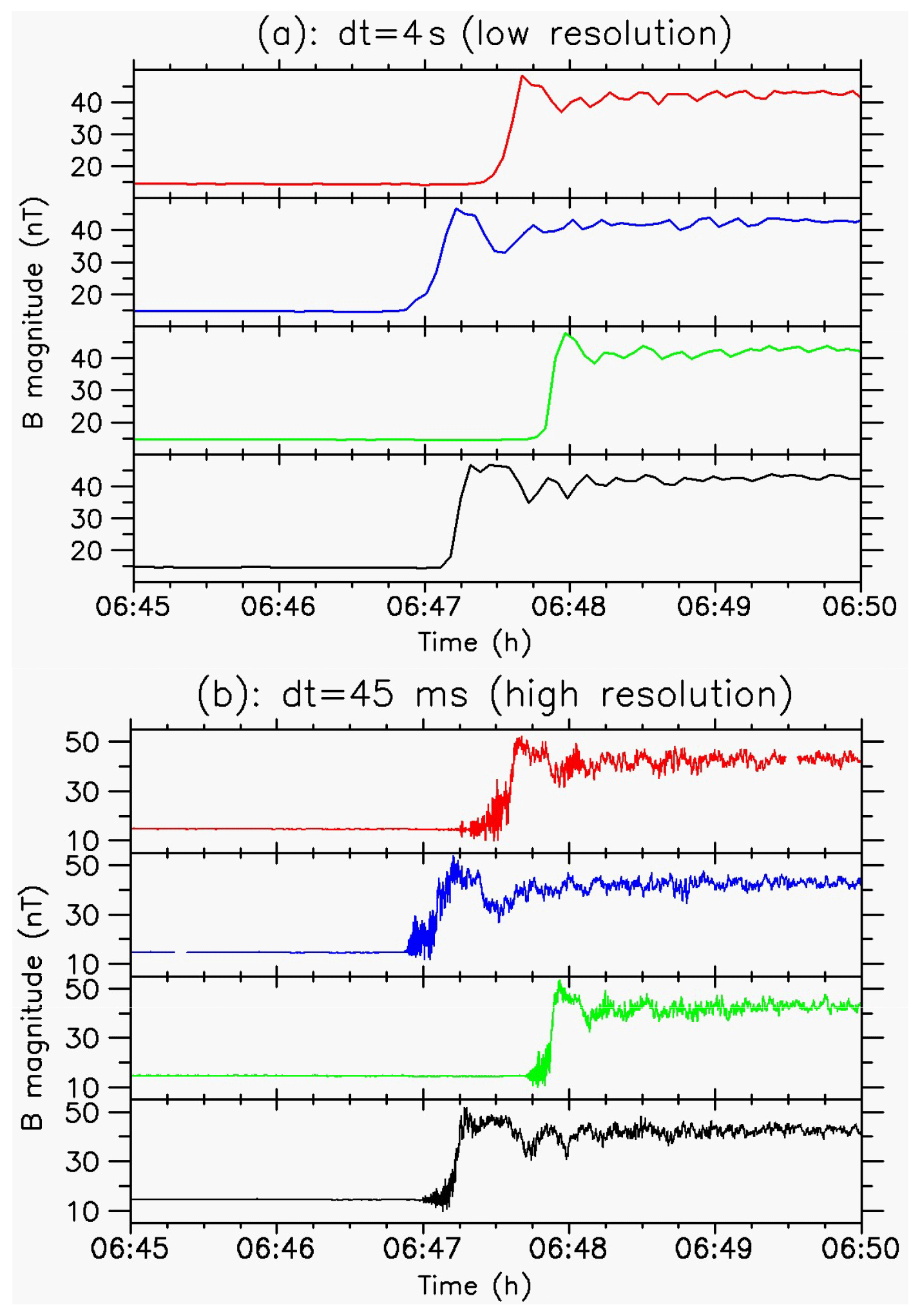
Figure 1 Total magnetic field amplitude measured versus time during the same shock crossing by each of the four Cluster satellites on 22 April 2001 around 06:47 UT (M_A=3.8; β_i=0.04 so that $v_{\mathrm{sh}}/v_{\mathrm{thi}}\gg \mathrm{1}$, ${\mathit{\theta }}_{B_n}=\mathrm{89}$^∘). The same measurement is performed at low time resolution (dt=4 s in panel a) and high time resolution (dt=45 ms in panel b).

2.2 Methodology

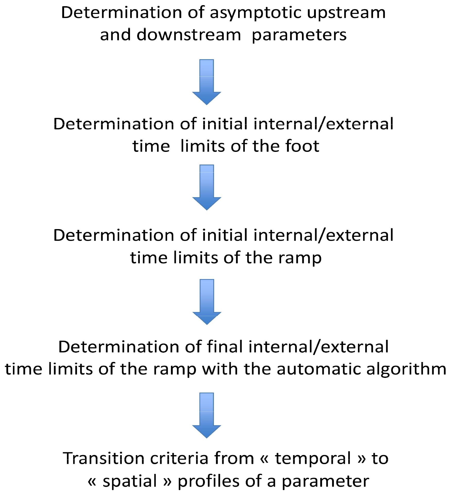
We detail for the first time a new methodology to carefully analyze experimental data for the study of supercritical quasi-perpendicular shocks. The step-by-step analysis method we have developed is illustrated in Fig. 2 and is conceptually straightforward. First, for each satellite, the temporal extension of each microstructure of the shock front is determined in the time series of the magnetic field. For each of them, beginning and end times are first estimated by visual inspection. For many previous studies in the literature, the process usually stops at this level, leaving the possibility of strong bias. Here, this first step is made only to initialize later automatic algorithms which will be used eventually to determine spatial error bars (both for the outer and inner edge of each microstructure). For each beginning or end time of a microstructure, we get a first estimate of an error bar on it by defining two associated times: one time (e.g., t_a) when the spacecraft has already likely entered the shock front or left the previously estimated microstructure and a second time (e.g., t_b) when the spacecraft is inside the present microstructure for sure. The order of these two times obviously depends on whether there is an inbound or outbound bow shock crossing. This may appear arbitrary and occasionally difficult to estimate, but experience shows that the risk to miss the real beginning and end times inside the defined interval is very low. Different stages of the present methodology are summarized in Fig. 2 and are detailed below.

Figure 2 Different stages of the methodology (see text for details).

2.2.1 Determination of asymptotic upstream and downstream parameters

The determination of upstream parameters entails a steady asymptotic upstream interplanetary magnetic field (IMF) B₀ associated with each shock crossing by the four spacecraft. For highly perpendicular shocks, however, it is often possible to define an unperturbed upstream field on a timescale of around a few minutes. For each satellite, we must define an upstream time interval displaying a magnetic field quite steady both in components and magnitude. For each spacecraft $s/c_i$, where $s/c_i$ represents for spacecraft i among the Cluster quartet (where i=1 to 4), an average upstream field B_0i is computed. Its magnitude is shown in the lower horizontal green line in Fig. 3a for one example of a single spacecraft shock crossing. Again, an initial estimated time interval is obtained from the visual inspection of the time series. The time duration cannot be too long since the usual stability timescale of the IMF due to the intrinsic solar wind variability (turbulence and directional discontinuities) is rarely more than a few tens of minutes (e.g., Burlaga, 1971), which we can take as an upper limit Δt_u. In order to be physically reliable, Δt_u cannot be too short. One reasonable lower limit Δt_l is the time interval during which a solar wind parcel travels a distance of one ion inertial length (about 100 km usually) that is about 1 min typically, considering the mean spacecraft velocities are all unchanged within a reasonable range. In this purpose, the six relative angles θ_ij measured between upstream fields B_0i and B_0j for $s/c_i$ and $s/c_j$ with ($i,j=\mathrm{1}$ to 4) are computed. The upstream vector B_0i measured by satellite i must be as close as possible to the vector B_0j measured by another satellite j. If all angles θ_ij are less than 5^∘ (arbitrary value chosen herein from empirical considerations), then the procedure is pursued; otherwise, the upstream time intervals (where these θ_ij values are calculated) are automatically modified by slightly shifting and reducing them until the above constraint on θ_ij is satisfied. The shock event is rejected from the present analysis when the adjustment fails or is not satisfactory.

When possible, the use of a larger time interval improves the statistics. Using the initial estimate of Δt and constraining it to be between Δt_l and Δt_u, the best upstream interval corresponds to the lowest values of the standard deviations σ for both the magnitude and components of the field. Although this can be easily verified by visual inspection, it allows us to ensure the absence of any solar wind disturbance. The following step deals with the determination of a unique unperturbed ambient IMF B₀ for every shock crossing by the four-spacecraft constellation. First, it is necessary to compare the individual upstream fields B_0i. This determination of B₀ is of crucial importance for the present study since it impacts both the value of the shock Alfvén Mach number through the field magnitude used and the determination of the angle ${\mathit{\theta }}_{B{n}_{\mathrm{0}}}$ between B₀ and the global shock normal n₀. This is obviously the first possible source of error in the determination of both the upstream Alfvén velocity, the Alfvén and magnetosonic Mach numbers, and the angle ${\mathit{\theta }}_{B{n}_{\mathrm{0}}}$.

2.2.2 Determination of initial internal and external time limits of the foot

For each satellite, the standard deviations, σ, obtained above for the magnetic field components and magnitude allow for the determination of the time when the spacecraft penetrates inside the magnetic foot. We determine, for each component and magnitude, the time when it is above a 3σ threshold level and close to the initially estimated time of the entry into the foot obtained by visual inspection (t_a dashed blue line in Fig. 3a). Then, we select the “external” limit of this entry (t₁ in Fig. 3a) among these four times as the closest to the external estimate t_a, and we select the “internal limit” (t₂ in Fig. 3a) as the closest to the internal estimate t_b (dashed blue lines in Fig. 3a). The derived times, t₁ and t₂, then define the error bar of the foot entry in the time domain. For the present case, the visual estimate t_b nearly coincides with the time t₂ automatically determined. Moreover, the possible presence of solar wind or foreshock transients as well as a detached whistler wave packet must be avoided. The last case occurs quite often even in the nearly perpendicular configuration and can easily lead to a wrong determination. Also, solar wind transients are always possible, while foreshock transients may only be an issue for a more “oblique” configuration which is not addressed in the present study. Nevertheless, it is necessary to make a cautious post-visual inspection.

2.2.3 Determination of initial internal and external time limits of the ramp

Similarly, the initial estimated times of the other microstructures are labeled with letters, and the final times determined from the present methodology are labeled with numbers. The times t_c and t_d are the initial “visual” estimates for the exit from the foot and entry into the ramp, respectively. They will be only used for initializing the automated algorithm described below. A major caveat in many previous attempts to compute the ramp thickness in the literature is to include in the ramp the part of the magnetic field profile up to the maximum of the first overshoot. To avoid this and to define at least the first overshoot well, we need to determine a downstream (asymptotic) level which would be required, for instance, for checking the Rankine–Hugoniot conditions. For that purpose, it is necessary to define a downstream interval in the magnetosheath far enough from the consecutive overshoots or undershoots displaying a quasi-steady magnetic field. This choice is highly important and not always straightforward in the case of very close consecutive crossings (multiple crossings) where only an average over the region of the sequence of overshoots or undershoots will be estimated. When a “clean” time interval downstream from this overshoot or undershoot interval is available, the average values obtained for B magnitude and components can be compared to the values inside the overshoot or undershoot interval. If these values are in good agreement, the downstream interval is appropriate for the determination of the asymptotic value. It is then used to give an initial estimate (t_e, t_f) of the final time interval (t₅, t₆) for the exit from the ramp or entry into the overshoot by using ±5 % of the computed asymptotic value (which is arbitrary but appears to be a good empirical compromise). It should be mentioned that a 1σ level can also be determined here, but it will usually be large in this region (local microturbulence in the magnetosheath) and not appropriate for the present purpose. The two times (t_e, t_f) are again only used for initializing the next automated step.

2.2.4 Determination of final internal and external time limits of the ramp with the automatic algorithm

From the initial time estimates (t_c, t_d) and (t_e, t_f), the determination of the final times for the entry into and exit from the ramp, (t₃, t₄) and (t₅, t₆), respectively, is made with an automatic algorithm. In order to characterize a steep gradient, we perform a linear fit of the data points between t_c and t_f. The time range for the regression can vary on both sides. The process is initialized by the largest possible time interval with t₃=t_c and t₆=t_f. Then, the entry time can vary between t_c and t_d, while the exit time can vary between t_e and t_f. The choice of a linear fit mainly excludes any “pollution” of the ramp region by a part of the extended foot (around the upstream edge of ramp) and by downstream fluctuations around the overshoot (around the downstream edge of the ramp). The resulting time interval is associated with the best linear regression coefficient, and the bounding times (t_c and t_f) explored during the automatic procedure are kept to estimate the error bars. In other words, we impose t₃=t_c and t₆=t_f. The automatic procedure only defines t₄ and t₅ (internal limits of the ramp). Then, the crossing of the downstream asymptotic value closer to the first estimate defines the exit from the overshoot (nearly equivalent to the middle of the gradient between the first overshoot and the first undershoot, not shown in detail here). The times t₇ and t₈ for the exit from the first overshoot are defined in the same way as the entry (Fig. 3a). The time t_g shown by a vertical dashed blue line is – as for the other microstructures – simply the initial rough “visual” estimate and is just shown for reference for a later visual check.

For every shock crossing by the Cluster quartet, we make the same procedure for each satellite. The satellite that is associated with the steeper ramp from this analysis is used to arbitrarily define what is called the “reference satellite” for a shock crossing event. Then, we determine the middle time t_ramp,i of the ramp crossing time interval for each individual satellite i and the “reference time” for a shock crossing is simply this middle time t_ref for the arbitrarily chosen reference satellite. Next, we determine the shock velocity and normal from the four different middle times t_ramp,i and the four spacecraft positions in the GSE (Geocentric Solar Ecliptic ) frame by using the classical “timing method” (e.g., Schwartz, 1998; Horbury et al., 2001, 2002). This method works if the separation between the spacecraft is not too large (otherwise the hypothesis of a planar structure breaks down) and provided that the four spacecraft are not coplanar (otherwise the method fails) and that the shape of the tetrahedron is not very elongated (which is not the case for the present study). This method provides a global normal vector n₀ valid only at the length scale of the spacecraft tetrahedron (i.e., the largest inter-distance between two satellites) and at the temporal scale defined by the time interval between the first crossing and the last crossing among the four satellites. The error bars for the entry or exit times are used to determine an error bar for the normal vector. It must be mentioned that each local normal vector n_i for the crossing by $s/c_i$ can differ from the global n₀ because of the small-scale turbulence of the front (shock front ripples) but cannot be determined experimentally as reliably as n₀ by any classical single-spacecraft method. Moreover, as will be discussed later, we intend here to compare the values determined experimentally with simulation results for which the normal vector n₀ and thus the ${\mathit{\theta }}_{B{n}_{\mathrm{0}}}$ angle are globally defined for a shock front both averaged spatially perpendicular to the normal and in time (see Sect. 4.4). This will also conversely justify the averaging along the shock front made in the simulations (that will be described in Sect. 4.4). The local effect due to the variation of the local normal direction n_i with respect to B₀ (local curvature effect due to the shock rippling at a lower scale) is not analyzed in the present work.

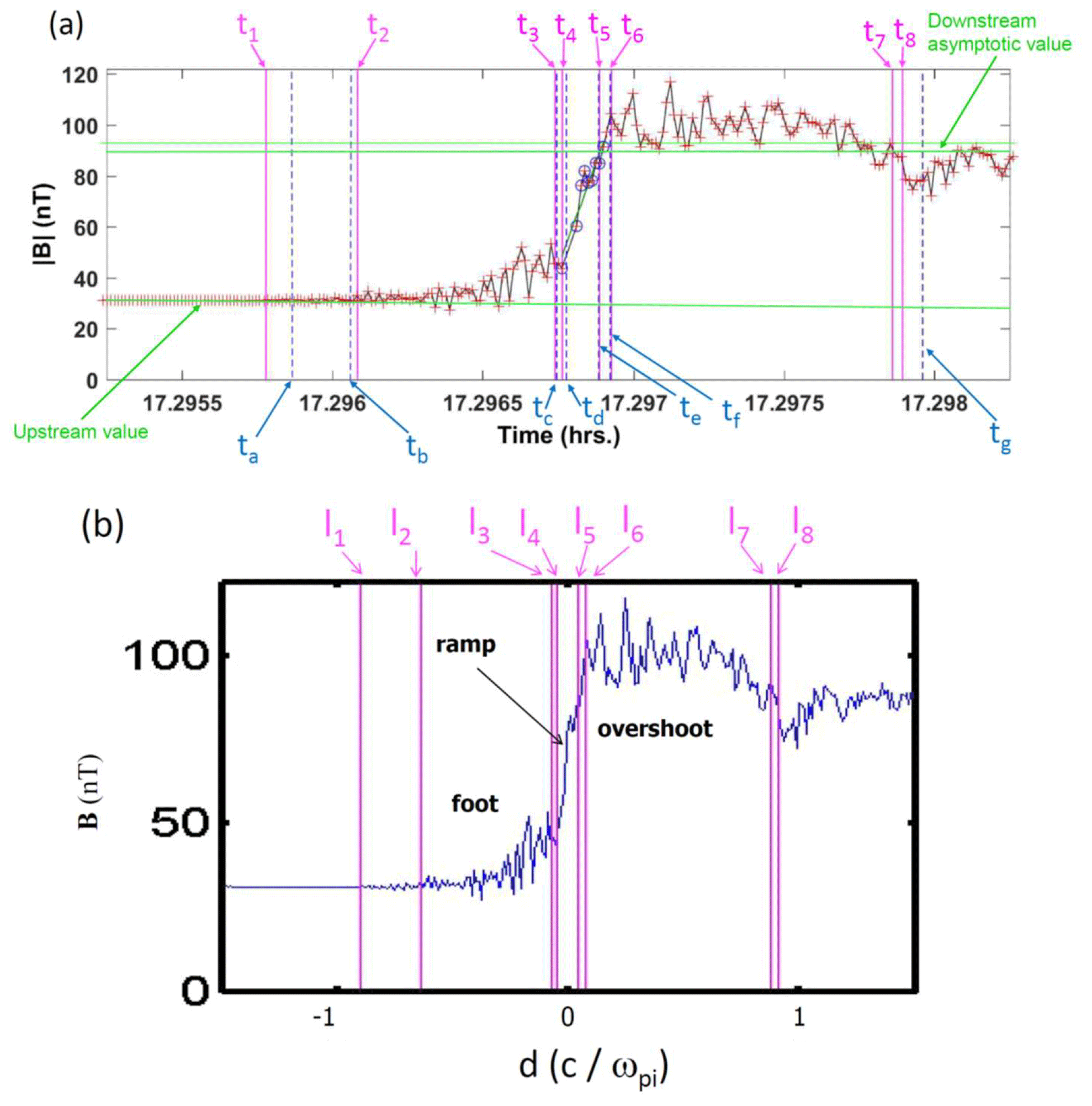
Figure 3 (a) Temporal profile of the magnetic field magnitude B for one satellite crossing only (measured by one of the Cluster satellites C1 on 31 March 2001 around 17:17:50 UT; times are shown as decimal hours). The individual data points are shown as red crosses; the green horizontal lines indicate the asymptotic upstream B₀ and downstream B_d±5 % B_d values. The initial time estimates are labeled with letters (t_a to t_g) and the final times determined from the automatic methodology are labeled with numbers (t₁ to t₈); (b) Corresponding spatial profile along the shock normal for the same B magnitude obtained from the time series of (a); the locations labeled with numbers (l₁ to l₈) have been deduced from the final times (t₁ to t₈) from (a). Adapted from Mazelle et al. (2010a).

2.2.5 Transition criteria from “temporal” to “spatial” profiles of a parameter

For all the shock front microstructures, the above analysis gives an “apparent” temporal extension along each satellite path and allows us to compare them between the four satellites. In every individual spacecraft frame, we compute an individual shock velocity vector. Since the spacecraft velocities in the Earth frame are typically around a few kilometers per second (km/s) as also found for many slowly moving shocks in the same frame, it is essential to also take these small spacecraft velocities into account. The major aim of the present analysis is to reconstruct a local spatial profile along the global shock normal n₀ as shown in Fig. 3b. For this purpose, the angle between each spacecraft i trajectory and n₀ has been used. Then, it is possible to measure the local physical thicknesses along n₀ of the microstructures of the shock front and compare them between the different satellites. It must be mentioned that the shock velocity determined by the four-spacecraft timing method here is an averaged velocity within the time interval separating the first and the last shock crossings. Then, it is supposed to be constant during this time interval and homogeneous over the spatial scale of the tetrahedron. One cannot preclude that the shock velocity can vary inside the considered time interval and that the shock motion is subject to some acceleration inward and/or outward. However, this possible effect can be assumed as weak if the temporal profiles of the shock crossing are quite similar in time series taken at low temporal resolution (such as in Fig. 1a). In contrast, when a sudden shock front acceleration or deceleration (due to a solar wind fluctuation) occurs between the crossings by two satellites, there is a clear signature in the time series (see in Fig. 4, derived from Fig. 1 in Horbury et al., 2002). Figure 4b and c are typical cases of observations which are eliminated from our present analysis. We use the same shock velocity in the Earth's frame for the four crossings to derive the spatial widths along the global normal n₀ for any case like in Fig. 4a.

Then, we can compare the obtained thicknesses of the shock microstructures with physical length values predicted either by theory or from numerical simulation results. It must be mentioned that using only time series can lead to wrong comparative classification of the observed crossings. A large angle between the spacecraft velocity vector and the shock front normal can produce a long crossing duration for a real very small physical thickness and will also produce a small shock speed. In summary, a particular precaution is necessary to avoid conclusions deduced exclusively from the temporal profiles, especially in the selection process which is often based solely on the steepness of the temporal gradient in the literature.

In order to have a qualitative check of the determination of the global normal n₀, the time series of the component B_n of the instantaneous magnetic field along this normal is systematically examined. First, this normal component is supposed to be conserved on both sides of the shock front. Second, for a nearly perpendicular shock, this component is expected to vanish (exactly zero for 90^∘ shock) upstream from the shock front and inside the ramp, since the vector of the magnetic field is supposed to be strictly along the shock front. Figure 5 displays the temporal evolution of B_n for a shock front crossing on 31 March 2001 around 17:38 UT for one of the four satellites (magenta lower curve) in comparison with the total magnitude B (black upper curve). For this shock, the ${\mathit{\theta }}_{B_n}$ angle is about 86^∘. If one takes into account the fluctuations observed in and around the ramp, the conservation in the front is well respected, and the upstream value is also very low as expected for a nearly perpendicular case. The downstream evolution in the overshoot is also consistent with expected oscillations around the average downstream value (e.g., Kennel et al., 1985).

Figure 4 Three examples of the total magnetic field amplitude measured versus time by each of the four Cluster satellites during three different shock crossings at a resolution of five vectors per second. Panel (a) illustrates a good (selected) example of a clean and sharp shock, while panels (b) and (c) have been rejected in our selection since the shock either exhibits a complex and disturbed profile (b) or the shock certainly suffers an important acceleration (c) as shown between the profiles measured by the four spacecraft (inspired from Horbury et al., 2002).

3 Analysis of individual shock crossings

3.1 One typical case

A typical example of the spatial profiles is shown in Fig. 6. It is obtained for one supercritical quasi-perpendicular shock crossing by Cluster on 31 March 2001 at 17:38 UT (${\mathit{\theta }}_{B_n}=\mathrm{86}\pm \mathrm{2}$^∘, M_A=4.1, β_i=0.05) when the $s/c$ separation was about a few ion inertial lengths $c/{\mathit{\omega }}_{\mathrm{pi}}$ (herein $c/{\mathit{\omega }}_{\mathrm{pi}}$ = 80–120 km, typically). The profiles are ordered by the sequence of crossings starting from satellites C4 to C3 (top to bottom in Fig. 6a and b). The relative locations of the four $s/c$ defined at the reference time given by satellite C4 (see Sect. 2.2) are represented in the plane containing both the X_GSE direction and the normal n₀ (Fig. 6c) and in the plane perpendicular to the normal n₀ (Fig. 6d).

In a first approach, the differences between the $\mathrm{4}s/c$ spatial profiles in Fig. 6b are quite obvious, particularly for the magnetic foot and the overshoot widths; however, these are less evident for the ramp. We emphasize that all upstream conditions remain unchanged for all four satellites. As a consequence, this shows the strong variability of the quasi-perpendicular shock front itself. We stress that the ramp widths can be very narrow and can reach values as low as a few electron inertial lengths with the thinnest one reaching $\mathrm{5}c/{\mathit{\omega }}_{\mathrm{pe}}$ for satellite C4. This result strongly disagrees with the typical scale length of the ramp commonly considered around $c/{\mathit{\omega }}_{\mathrm{pi}}$ (e.g., Russell and Greenstadt, 1979; Scudder et al., 1986; Bale et al., 2005), although it is in very good agreement with some “exceptional” ISEE results (Newbury and Russell, 1996; Newbury et al., 1998) as well as theoretical studies predicting the existence of small scales in quasi-perpendicular shocks as a signature of the front nonstationarity or results issued from PIC numerical simulations (Lembège and Dawson, 1987; Lembège and Savoini, 1992; Lembège et al., 1999, 2013a, b; Scholer et al., 2003; Marcowith et al., 2016, and references therein).

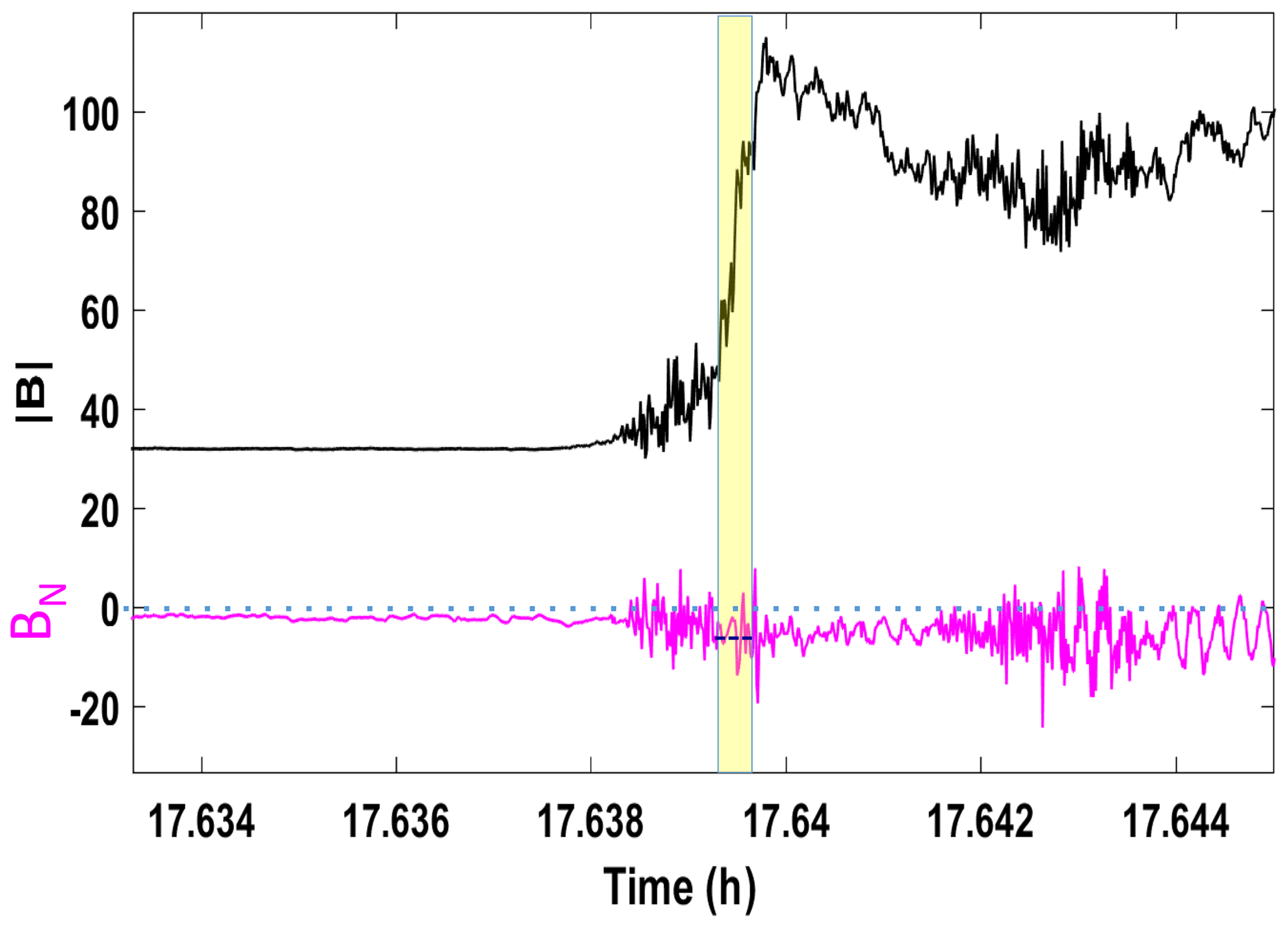
Figure 5 Time variation of the B amplitude and of its associated B_n normal component (used to verify the criterion on the normal component; see Sect. 2.2) on 31 March 2001 around 17:38 UT, where M_A=4.1, ${\mathit{\theta }}_{B_n}$ = 86^∘ ± 2^∘, and β_i=0.04; time is in decimal hour. The vertical yellow bar indicates the identified location of the ramp.

This nonstationarity can also be shown in the content of Fig. 6. The C3 and C4 satellite locations are almost aligned with the direction n₀ (Fig. 6c) and are close to each other (over a distance of less than $c/{\mathit{\omega }}_{\mathrm{pi}}$) in the plane perpendicular to n₀ (Fig. 6d). If the shock front was stationary, after propagating from C4 to C3, the profiles are expected to be nearly identical, but they appear significantly different. For instance, the spatial ramp thickness for C3 is about twice the one for C4, and the shape and thickness of the overshoot are also very different. Moreover, C2 and C1 locations are not far enough to be along the n₀ direction (Fig. 6c), but they depart from each other in the perpendicular plane to n₀ (i.e., along the shock front) by several $c/{\mathit{\omega }}_{\mathrm{pi}}$ (Fig. 6d). The differences mentioned here can be related to the shock front nonuniformity due to its rippling; the impact of this rippling on the front variations will be analyzed in a future work.

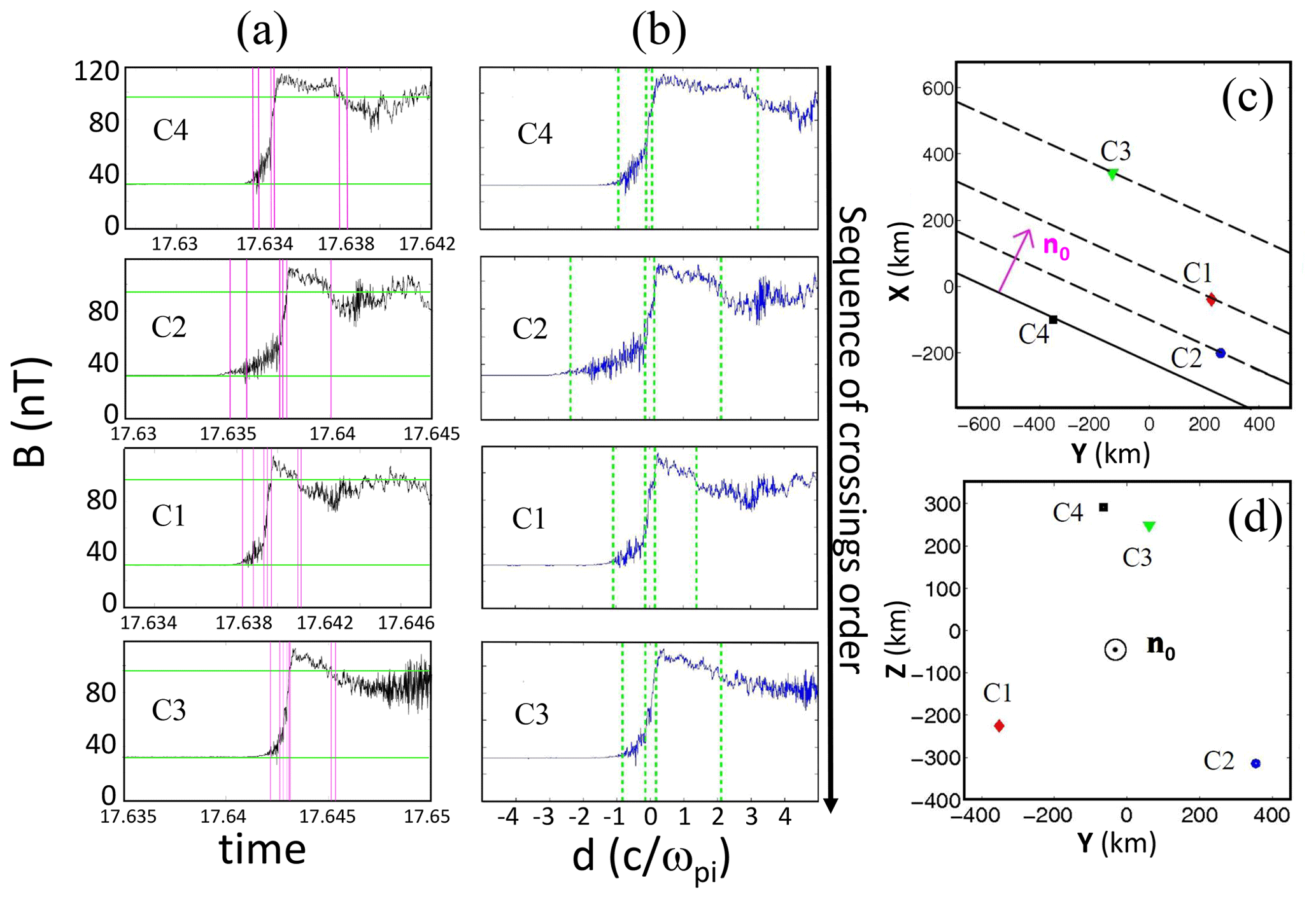
Figure 6 Time and spatial profiles along the normal of the magnetic field magnitude for the shock crossing on 31 March 2001 at 17:38 UT are shown in (a) and (b), respectively. For this shock crossing, v_sh=18 km/s, M_A=4.1, ${\mathit{\theta }}_{B_n}=\mathrm{86}$^∘ ± 2^∘, and β_i=0.05. The locations of the four Cluster satellites for the event displayed at the reference time t_ref defined for satellite C4 (see text) are reported within the plane defined by X_GSE and the normal n₀ (c), and within the plane perpendicular to n₀ (d). (Panels (b), (c), and (d) are issued from Figs. 3 and 4 of Mazelle et al. (2010a).)

3.2 Impact of the shock velocity

A careful determination of the shock velocity is necessary in order to discuss the physical spatial thicknesses of the shock front microstructures. This also means that it is not possible to consider only time series to discuss the relative properties of different shock crossings. Moreover, as already stated previously, the time resolution of the data needs to be considered before any conclusion. This is illustrated in Fig. 7. The left part shows the time series of the magnetic field components and magnitude for two shock front crossings and for two different time resolutions each (panels a1 and b1): the highest available resolution (15 or 60 ms depending on the mode) and the spin resolution of 4 s. These two shocks have been chosen as they are characterized with similar parameters ${\mathit{\theta }}_{B_n}$, M_A, and β_i. The first shock a (panel a1) is a slow-moving shock with a velocity of about 11 km/s, while shock b (panel b1) is a fast-moving shock with a velocity of about 78 km/s. When considering the lowest time resolution (averaged data on 4 s), the two profiles in the upper plots of panels a1 and b1 appear very similar. If only data with this time resolution were considered, one should have concluded at first glance that the two shock crossings are very similar and display very similar properties with relatively smooth time gradients of a similar shape. But, the highest time resolution on the lower panels reveals the large difference between shock profiles when changing the data sampling: shock b appears steeper than shock a. Moreover, for shock a, the gradient remains nearly unchanged with only superimposed higher-frequency fluctuations which are not observed upstream from the sharp front displayed by shock b. The full shock properties are revealed only if the spatial profiles, as shown on panels a2 and b2, are considered. The general shapes of the shock front microstructures are very similar for the two shocks, but the steeper spatial ramp is obtained for shock a, while shock b displays a ramp spatial thickness more than twice that of shock a (right-hand panels a2 and b2, respectively). Moreover, it also reveals that the structure of the shock is better sampled up to much higher frequencies for a slow shock velocity. In the spacecraft frame, any instrument like the magnetometer uses a constant sampling frequency and thus obviously measures much fewer measurement points inside any shock front microstructure when this one is propagating faster. This example illustrates quite well the advantages of the methodology developed in the present study to correctly address the spatial scales of a shock front and the careful precaution to keep in mind when analyzing only the temporal shock profiles.

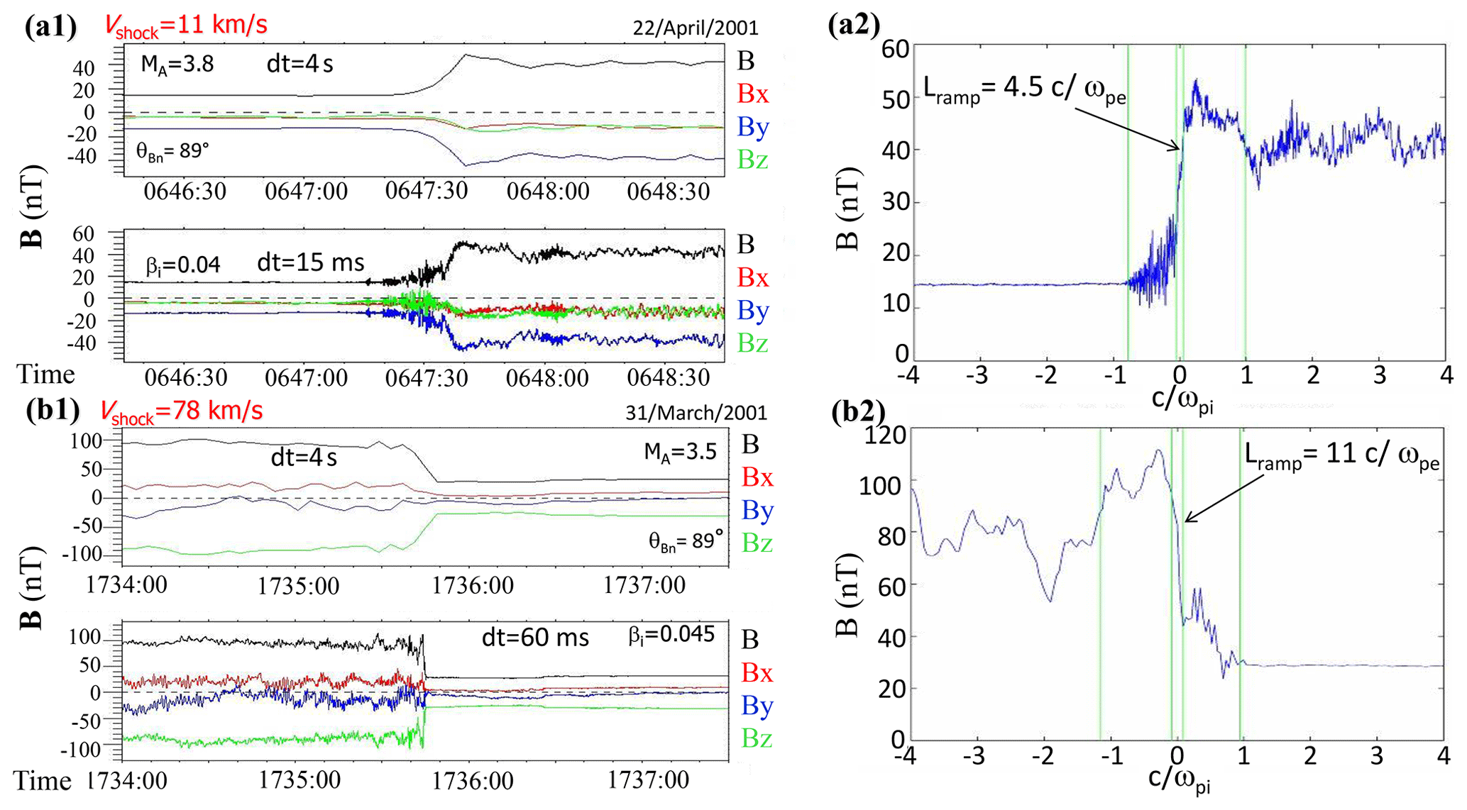
Figure 7 Comparison of a slow-moving shock (a1 and a2, where v_sh=11 km/s, M_A=3.8, ${\mathit{\theta }}_{B_n}=\mathrm{89}$^∘, and β_i=0.04) and a rapid shock (b1 and b2, where v_sh=78 km/s, M_A=3.5, ${\mathit{\theta }}_{B_n}=\mathrm{89}$^∘, and β_i=0.045) defined for low- (dt=4 s) and high-resolution rates (dt=15 or 60 ms). Panels (a1) and (b1) provide the temporal profiles of the total magnetic field amplitude defined, respectively, for C1 and C3, while panels (a2) and (b2) provide correspondingly the spatial profiles of the measured magnetic field (the distance is normalized with respect to the ion inertial length defined upstream). The spatial origin corresponds to the location at the middle time of the ramp crossing interval for each satellite.

4 Statistical analysis

4.1 Selection criteria

An analysis similar to the one described in Sect. 3 has been performed for a list of shocks after a severe selection procedure. Several criteria have been used: (i) limitation to shocks normal direction ${\mathit{\theta }}_{B_n}$ approaching 90^∘ as much as possible (more than 75^∘) in order to avoid more complex mechanisms which take place at oblique shocks (Lembège and Savoini, 1992; Lembège et al., 2004; Marcowith et al., 2016), (ii) existence of well-defined upstream and downstream ranges for each of the $\mathrm{4}s/c$, (iii) stability of the upstream averaged magnetic field from one $s/c$ to another, (iv) validity of the normal determination by checking the weak variability of the normal field component B_n around the ramp and low value of $B_n/\left|\mathit{B}\right|$ upstream for ${\mathit{\theta }}_{B_n}$ close to 90^∘, (v) availability of all data necessary to compute the shock parameters, and (vi) a maximum spacecraft separation distance limited to a few $c/{\mathit{\omega }}_{\mathrm{pi}}$ between the four spacecraft in order to consider the crossing of a same “individual” shock front by all Cluster spacecraft. From an initial ensemble of 455 shock crossings (including essentially data for 2001 and 2002 for which spacecraft separation distances are all small enough), only 24 shock events have been selected after the validation of the aforementioned criteria. This implies a detailed analysis of 96 individual shock crossings. Figure 8 displays the distributions of four main parameters ${\mathit{\theta }}_{B_n}$, M_A, β_i, and $v_{\mathrm{sh}}/v_{\mathrm{thi}}$ (see Sect. 1). For the selected shock crossings, the ${\mathit{\theta }}_{B_n}$ values extend from almost 90 to 75^∘ but mostly above 84^∘ (80 %), the M_A values of the resulting shocks are equally distributed from 2 to 6.5, the ratio $v_{\mathrm{sh}}/v_{\mathrm{thi}}$ between 2 and 30 with a peak within the range 12–24, and β_i extends from very low values to 0.6 but with 67 % of values less than 0.1.

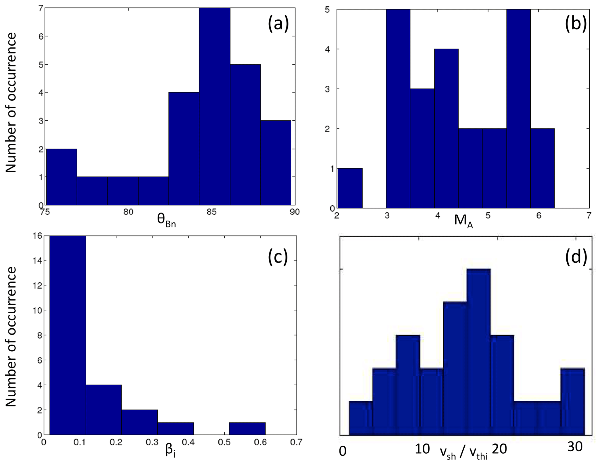
Figure 8 Distribution of the 96 (selected) shock crossings versus (a) the angle ${\mathit{\theta }}_{B_n}$ (defined between the shock normal direction and the upstream magnetic field), (b) the Alfvén Mach number ($M_{\mathrm{A}}=V_{\mathrm{sw},\mathrm{n}}/v_{\mathrm{A}}$, where V_sw,n is the solar wind bulk velocity component defined along the shock normal, and v_A is the upstream Alfvén velocity, respectively), (c) the ratio β_i (between the ion thermal pressure and the magnetic pressure), and (d) the ratio $v_{\mathrm{sh}}/v_{\mathrm{thi}}$ where v_sh is the velocity of the shock front defined in the rest plasma frame (to be compared with present simulation results), and v_thi is the upstream solar wind proton velocity.

4.2 Ramp thickness

The obtained ramp thickness distribution shown in Fig. 9a appears Gaussian, indicating that most of the shocks are associated with a narrow ramp. Interestingly, the distribution reveals a cutoff mark at $c/{\mathit{\omega }}_{\mathrm{pi}}$. Figure 9b displays the thinnest ramp found among each quartet of crossings for each individual shock versus ${\mathit{\theta }}_{B_n}$. No simple relation emerges. However, many observed thinnest ramps have a width of less than $\mathrm{5}c/{\mathit{\omega }}_{\mathrm{pe}}$, and the magnetic ramps thickness tends to reach low values when approaching 90^∘. Figure 9c and d display scatter plots of all ramp thicknesses versus ${\mathit{\theta }}_{B_n}$ and M_A, respectively; for clarity, individual error bars are not reported on the figure.

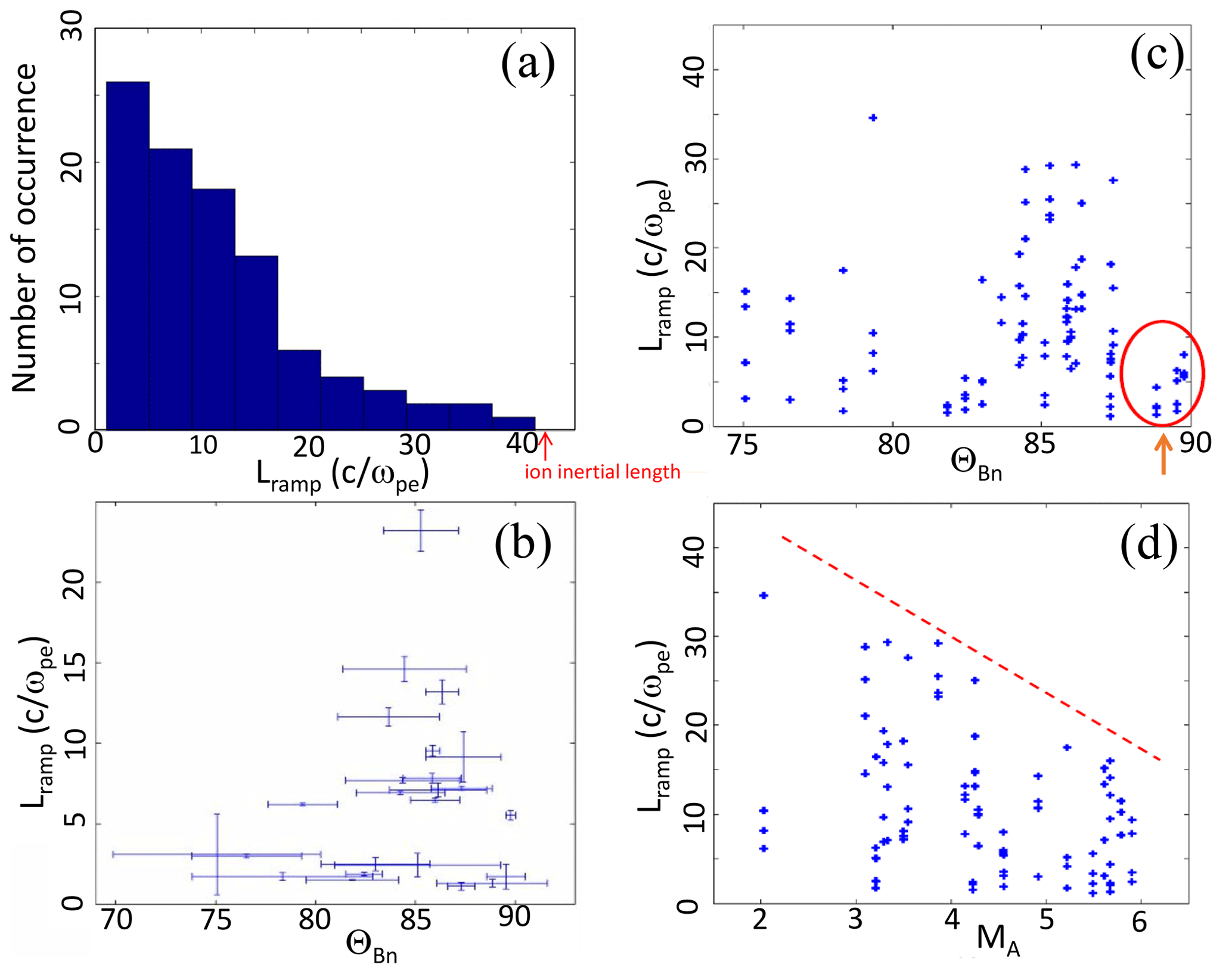
Figure 9 (a) Distribution of all ramp thicknesses measured by the four Cluster satellites during the 24 shock crossings (total covers 96 individual crossings). (b) Distribution of the thinnest ramp thickness observed versus the angle ${\mathit{\theta }}_{B_n}$ (defined between the shock normal direction and the upstream magnetic field); each thinnest thickness is selected among the four measurements made by the four satellites during the crossing of the same shock. Panels (a) and (b) are derived from Figs. 5 and 6 of Mazelle et al. (2010a). Distribution of all ramp thicknesses (all spacecraft measurements mixed) versus (c) the angle ${\mathit{\theta }}_{B_n}$ and (d) the Alfvén Mach number ($M_{\mathrm{A}}=V_{\mathrm{sw},\mathrm{n}}/v_{\mathrm{A}}$), respectively; V_sw,n and v_A are, respectively, the bulk solar wind velocity along the shock normal and the upstream Alfvén velocity. The ellipse in (c) focuses on results around ${\mathit{\theta }}_{B_n}=\mathrm{90}$^∘; the dashed line in (d) indicates the upper limit of the $L_{\mathrm{ramp}}/(c/{\mathit{\omega }}_{\mathrm{pe}})$ values.

Although Fig. 9c shows no clear dependence of the ramp width with ${\mathit{\theta }}_{B_n}$, it indicates that the narrowest ramps are associated with nearly perpendicular geometries as pointed out by the red arrow. Figure 9c also shows that the ramp thickness variation is not solely controlled by the shock geometry. It can vary a lot for a single value of ${\mathit{\theta }}_{B_n}$ except maybe when close to 90^∘. Moreover, the ramp thickness obtained from the analysis of a same crossing with each single $s/c$ appears inconsistent (up to a factor 7) although the upstream conditions remain similar. This illustrates quite well the signature of an intrinsic shock front nonstationarity. Figure 9d does not reveal any simple relation of the shock ramp thickness with M_A. It may only illustrate that the maximum observed thickness reduces as the Mach number increases, although the scatter plot and the statistics do not allow us to make any other conclusive result.

The statistics confirm the important result, shown in the individual case study of Sect. 3, that the magnetic field ramp of a supercritical quasi-perpendicular shock often reaches a few $c/{\mathit{\omega }}_{\mathrm{pe}}$. The time variability of scales observed for the same upstream conditions is also consistent with a signature of the front nonstationarity due to the self-reformation fed by the accumulation of reflected ions in agreement with PIC and hybrid simulation results (Lembège and Dawson, 1987; Biskamp et Welter, 1972; Lembège et al., 2004; Lembège and Savoini, 1992; Hellinger et al., 2002). Other mechanisms raising from the modified two-stream instability (triggered by the relative drift between incoming electrons and incoming ions within the foot region of the front) for oblique shocks (Scholer et al., 2003) may also be responsible for the nonstationarity of the shock front as discussed in Sect. 5.

4.3 Magnetic foot

The left panel of Fig. 10 displays the distribution of the magnetic foot thickness for the 96 shock crossings by any individual spacecraft versus the foot thickness (normalized with the upstream ion gyroradius ρ_ci), whereas the right panel shows the maximal thickness among the four satellites for each selected shock crossed by the quartet (labeled with the numbers on the horizontal axis) versus the foot thickness normalized with ρ_ci.

First, the distribution (Fig. 10a) clearly shows that the foot thickness is always found less than the upstream gyroradius. Second, most of the foot thicknesses (81 %) are found to be less than 0.4ρ_ci,us, and the median value is 0.2ρ_ci,us. Most of the observed shocks are characterized by a foot with a thickness ($L_{\mathrm{foot}}<\mathrm{0.1}{\mathit{\rho }}_{\mathrm{ci},\mathrm{us}}$), indicating that the foot width rarely reaches its maximal value. The literature provides different theoretical determinations of the foot thickness. Gosling and Robson (1985) used the results of Schwartz et al. (1983) to show that for an arbitrary angle ${\mathit{\theta }}_{B_n}$, the upstream extent of the foot is

$$\begin{array}{}\text{(1)}& \begin{array}{rl}d& ={\mathit{\rho }}_{\mathrm{ci}}\cos {\mathit{\theta }}_{\mathrm{vn}}[{\mathrm{\Omega }}_p{t}^{\prime }\left(\mathrm{2}{\cos }^{\mathrm{2}}{\mathit{\theta }}_{B_n}-\mathrm{1}\right)\\ & +\mathrm{2}{\sin }^{\mathrm{2}}{\mathit{\theta }}_{B_n}\sin {\mathrm{\Omega }}_p{t}^{\prime }],\end{array}\end{array}$$

where

$$\begin{array}{}\text{(2)}& \cos {\mathrm{\Omega }}_p{t}^{\prime }={\displaystyle \frac{\mathrm{1}-\mathrm{2}{\cos }^{\mathrm{2}}{\mathit{\theta }}_{B_n}}{\mathrm{2}{\sin }^{\mathrm{2}}{\mathit{\theta }}_{B_n}}}\end{array}$$

and θ_vn is the angle between the shock normal and the upstream solar wind velocity vector.

Another determination was given by Livesey et al. (1984) as

$$\begin{array}{}\text{(3)}& d=\mathrm{0.68}{\mathit{\rho }}_{\mathrm{ci},\mathrm{us}}\cos {\mathit{\theta }}_{\mathrm{vn}}{\sin }^{\mathrm{2}}{\mathit{\theta }}_{B_n}.\end{array}$$

For a strictly perpendicular shock $({\mathit{\theta }}_{B_n}=\mathrm{90}{}^{\circ })$ and a normal incident upstream solar wind (${\mathit{\theta }}_{\mathrm{vn}}=\mathrm{0}{}^{\circ })$, the foot width reaches the distance for a reflected ion at the time of its turn-around defined by $\mathrm{d}{x}_n/\mathrm{d}t=\mathrm{0}$, where x_n is the coordinate of the ion along the normal, given by Woods (1969, 1971):

$$\begin{array}{}\text{(4)}& d=\mathrm{0.68}{\mathit{\rho }}_{\mathrm{ci},\mathrm{us}}.\end{array}$$

The values of d obtained from Eqs. (1)–(2) are shown by red points in Fig. 10b for each shock event. For each event, the blue value with error bar is the largest experimental foot thickness for one among the four satellites. The horizontal dashed light blue line shows the theoretical value given by Eq. (4) and clearly stresses that the maximal experimental foot thickness is usually below the 90^∘ critical value and the value obtained from the experimental derivation of ${\mathit{\theta }}_{B_n}$ and θ_vn (considering the error bars). Thus, for each specific shock crossing and associated parameters, the above two theoretical values which are supposed to be fixed by the two aforementioned angles (and thus not varying with time) can be generally considered an upper bound of the observed “instantaneous” foot thickness.

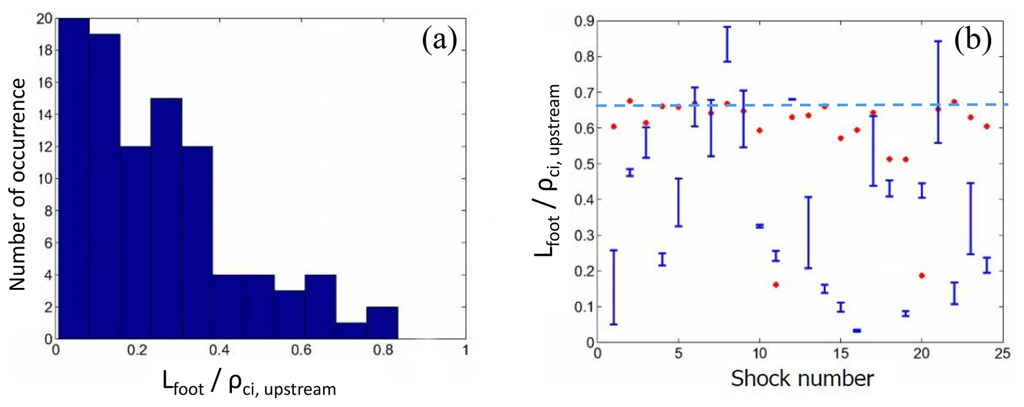
Figure 10 (a) Distribution of the 96 shock crossings versus the foot thickness (normalized versus the upstream ion gyroradius ρ_ci,upstream). (b) Distribution of the largest experimental foot thickness (normalized versus the upstream ion gyroradius ρ_ci,upstream) for every shock event; the vertical bars correspond to the error estimate made on the measured values in blue, and the red dots correspond to the upper-bound values, i.e., the theoretical values obtained from Eqs. (1)–(3) of Sect. 4.3 (Eq. 3 of Gosling and Robson, 1985). For reference, the value $L_{\mathrm{foot}}/{\mathit{\rho }}_{\mathrm{ci},\mathrm{upstream}}=\mathrm{0.68}$ defined for ${\mathit{\theta }}_{B_n}=\mathrm{90}$^∘ (Woods, 1971) is indicated by the light blue horizontal dashed line in (b).

4.4 Comparison with numerical simulation results

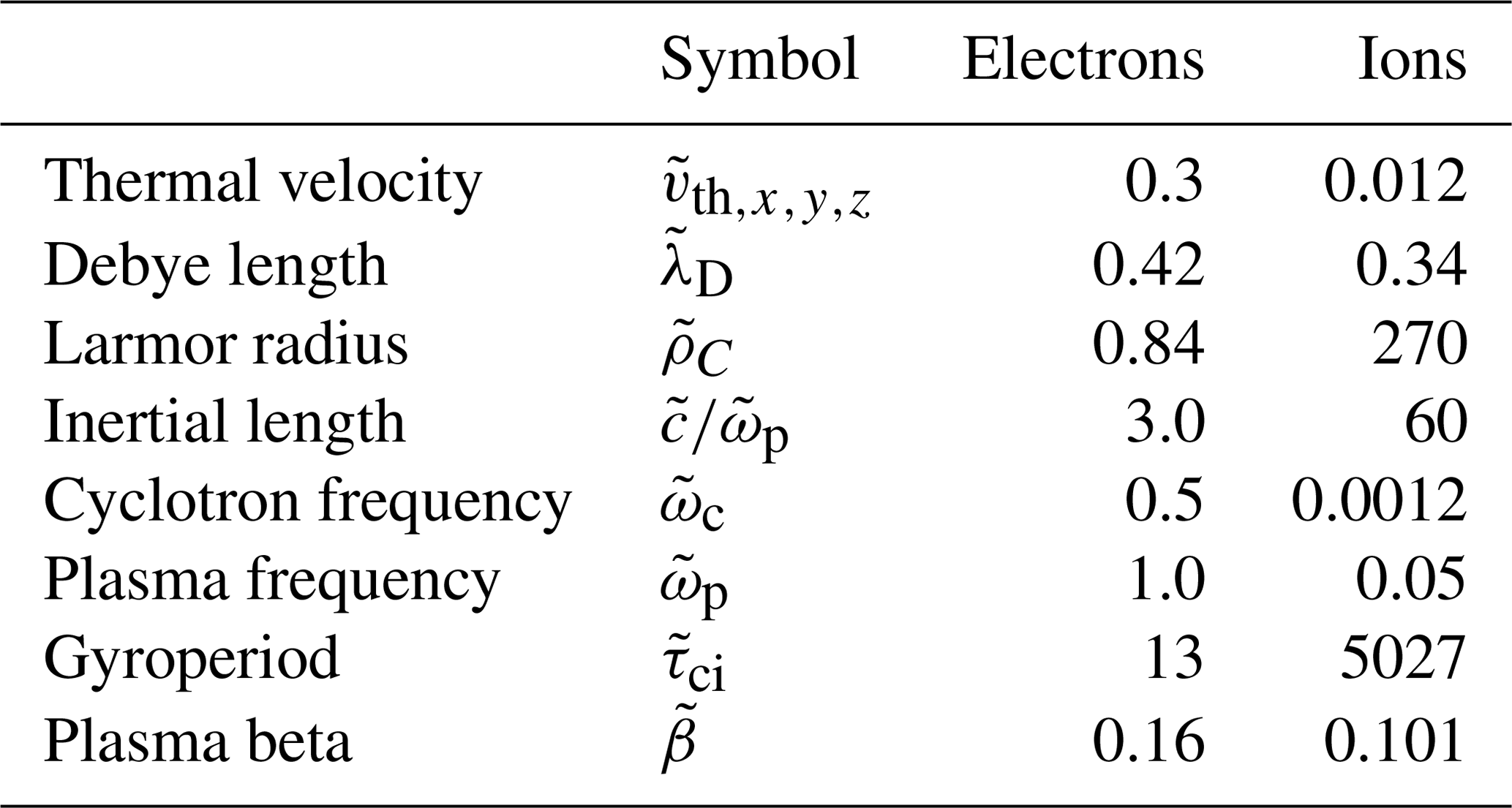
To compare more precisely with numerical simulation results, two-dimensional PIC simulations (where both ions and electrons are treated as individual macroparticles) have been performed like those of previous studies (Lembège and Savoini, 1992; Lembège et al., 2009), where the planar shock is initialized by a magnetic piston (applied current pulse). Therefore, the shock geometry is always defined in the upstream frame: the shock propagates along the x direction. Periodic conditions are used along the direction of the planar shock front (y axis). Herein, the shock is strictly perpendicular (${\mathit{\theta }}_{B_n}=\mathrm{90}$^∘) where the upstream magnetostatic field B₀ is along the z axis and propagates within the (x−y) simulation plane; this perpendicular shock is used as a reference case. All quantities are dimensionless, are indicated by a tilde “∼”, and are normalized as follows: the spatial coordinate is $\stackrel{\mathrm{̃}}{x}=x/\mathrm{\Delta }$; velocity $\stackrel{\mathrm{̃}}{v}=v/\left({\mathit{\omega }}_{\mathrm{pe}}\mathrm{\Delta }\right)$; time $\stackrel{\mathrm{̃}}{t}={\mathit{\omega }}_{\mathrm{pe}}t$, electric field $\stackrel{\mathrm{̃}}{E}=eE/\left(m_e{\mathit{\omega }}_p^{\mathrm{2}}\mathrm{\Delta }\right)$; and magnetic field $\stackrel{\mathrm{̃}}{B}=eB/\left(m_e{\mathit{\omega }}_p^{\mathrm{2}}\mathrm{\Delta }\right)$. The parameters e, m_e, Δ, and ω_pe are, respectively, the electric charge, the electron mass, the numerical grid size, and the electron plasma frequency. These definitions are identical to those used in previous 1D PIC (Lembège and Dawson, 1987) and 2D PIC simulations (Lembège and Savoini, 1992). The plasma conditions and shock regime used herein are similar to those used in Lembège et al. (2009). All basic parameters are summarized as follows: the plasma simulation box has 6144×256 grids with a spatial resolution $\mathrm{\Delta }=\mathrm{\Delta }x=\mathrm{\Delta }y=\mathrm{\Delta }z=\mathrm{1}/\mathrm{60}$ ($\stackrel{\mathrm{̃}}{c}/{\stackrel{\mathrm{̃}}{\mathit{\omega }}}_{\mathrm{pi}}$) = $\mathrm{1}/\mathrm{3}(\stackrel{\mathrm{̃}}{c}/{\stackrel{\mathrm{̃}}{\mathit{\omega }}}_{\mathrm{pe}})$ (where $\stackrel{\mathrm{̃}}{c}/{\stackrel{\mathrm{̃}}{\mathit{\omega }}}_{\mathrm{pi}}$ and $\stackrel{\mathrm{̃}}{c}/{\stackrel{\mathrm{̃}}{\mathit{\omega }}}_{\mathrm{pe}}$ are the upstream ion and electron inertial lengths, respectively), which is high enough to involve all microstructures of the shock front. Initially, the number of particles per cell is 4 for each species. Velocity of light $\stackrel{\mathrm{̃}}{c}=\mathrm{3}$, and mass ratio of proton and electron $M_{\mathrm{i}}/m_{\mathrm{e}}=\mathrm{400}$. To achieve reasonable run times and simulation domains, a ratio of ${\stackrel{\mathrm{̃}}{\mathit{\omega }}}_{\mathrm{pe}}/{\stackrel{\mathrm{̃}}{\mathit{\omega }}}_{\mathrm{ce}}=\mathrm{2}$ has been used as in Hada et al. (2003) and Scholer and Matsukiyo (2004). The electron-to-ion temperature ratio is $T_{\mathrm{e}}/T_{\mathrm{i}}=\mathrm{1.58}$; upstream ions and electrons are isotropic so that ${\stackrel{\mathrm{̃}}{v}}_{\mathrm{thi}}={\stackrel{\mathrm{̃}}{v}}_{\mathrm{thi},x,y,z}$ and ${\stackrel{\mathrm{̃}}{v}}_{\mathrm{the}}={\stackrel{\mathrm{̃}}{v}}_{\mathrm{the},x,y,z}$, respectively. The ambient magnetic field is ${\stackrel{\mathrm{̃}}{B}}_{\mathrm{0}}=\mathrm{1.5}$. The shock has an averaged alfvénic Mach number $M_{\mathrm{A}}={\stackrel{\mathrm{̃}}{v}}_{\mathrm{shock}}/{\stackrel{\mathrm{̃}}{v}}_{\mathrm{A}}=\mathrm{5.06}$, where the upstream Alfvén velocity ${\stackrel{\mathrm{̃}}{v}}_{\mathrm{A}}$ is equal to 0.075, and the shock velocity ${\stackrel{\mathrm{̃}}{v}}_{\mathrm{shock}}=\mathrm{0.38}$. The ratio $\stackrel{\mathrm{̃}}{\mathit{\beta }}$ of upstream plasma thermal pressure to magnetic field pressure is taken as ${\stackrel{\mathrm{̃}}{\mathit{\beta }}}_{\mathrm{i}}=\mathrm{0.10}$ for protons and ${\stackrel{\mathrm{̃}}{\mathit{\beta }}}_{\mathrm{e}}=\mathrm{0.16}$ for electrons. For these initial conditions, all other upstream plasma parameters are detailed in Table 1 for both electrons and protons.

In present plasma conditions, cycles of the shock front self-reformation are shown as in previous studies (Lembège and Dawson, 1987; Lembège and Savoini, 1992; Lembège et al., 2009). An enlarged view of the time stack plot of the (y-averaged) main magnetic field component is shown over one cycle in Fig. 11a. Note that the local direction of the front normal versus the upstream magnetostatic field is varying along a front ripple. Then, considering an average along the shock front (y axis) is equivalent to averaging over these local normal directions and agrees with the method used in experimental data for determining the normal direction of the shock front crossed by the Cluster tetrahedral configuration for small satellite inter-distance (i.e., average over local normal directions given individually by each satellite).

As shown in previous studies, the self-reformation is mainly characterized by (i) a strong cyclic magnetic field amplitude variation at the overshoot with a time period ${\stackrel{\mathrm{̃}}{\mathit{\tau }}}_{\mathrm{ref}}$ (=1523) on the order of $\mathrm{1}/\mathrm{3}{\stackrel{\mathrm{̃}}{\mathit{\tau }}}_{\mathrm{ci}}$ (where ${\stackrel{\mathrm{̃}}{\mathit{\tau }}}_{\mathrm{ci}}=\mathrm{5027}$ is the upstream ion cyclotron period) so that several self-reformations can take place within one upstream ion cyclotron period; (ii) a temporal anticorrelation of the B amplitude measured at the foot and at the overshoot, respectively, and (iii) a strong time variability of the shock front width. These features persist quite well even when using a realistic mass ratio as shown by Lembège and al. (2013a, b); in particular, the self-reformation cyclic period does not depend almost on the mass ratio. Moreover, the features of the other self-reformation process due to the MTSI (for slightly oblique shocks, see Sect. 1) also persist for realistic mass ratio as shown by Scholer and al. (2003).

Table 1 Upstream plasma parameters defined for the 2D PIC simulation.

4.4.1 Results on the ramp thickness

Herein, the spatial ramp width is identified within the shock front by a linear fit defined in the steepest part of the magnetic field gradient (Fig. 11b). However, the procedure to define this width slightly differs from that used for Cluster experimental data in Sect. 2. Presently, its lower bound (dashed line B) is defined where the B amplitude departs clearly (due to the foot region) from this linear fit. On the other hand, its upper bound (dashed line C) is defined where the B profile departs clearly (due to the proximity of the overshoot) from this linear fit. We do not use the overshoot as the upper bound since it is polluted by reflected ions as these gyrate and penetrate downstream after being once reflected at the ramp (Leroy et al., 1982); then this would overestimate the ramp width. On the other hand, let us note that using the mean downstream B amplitude as a reference (as done for experimental data analysis in Sect. 3) may be a source of inaccuracy when applied to the present numerical simulation results. Indeed, the size of the downstream region is not long enough to deduce a precise estimate of the averaged downstream B amplitude. In the B amplitude of Fig. 11b, these lower and upper bounds are, respectively, located at $\stackrel{\mathrm{̃}}{x}=\mathrm{3755}$ and 3745 which provides a ramp thickness ${\stackrel{\mathrm{̃}}{L}}_{\mathrm{ramp}}=\mathrm{10}$. Repeating the same measurement procedure at different times within the self-reformation cycle allows us to prove that the ramp thickness stays always very narrow around a (time-averaged) value of ${\stackrel{\mathrm{̃}}{L}}_{\mathrm{ramp}}=\mathrm{3}\stackrel{\mathrm{̃}}{c}/{\stackrel{\mathrm{̃}}{\mathit{\omega }}}_{\mathrm{pe}}$ (Fig. 11c); the width of the ramp is almost independent of time and of the strong fluctuations of the maximum B amplitude at the overshoot (not shown herein), which is mainly driven by reflected ions (Leroy et al., 1982). Since one has to compare statistical results of experimental observations with simulations, it is important to clarify the following points: (i) considering a perpendicular shock represents a reference case in the sense that the ramp is expected to be the thinnest for 90^∘, as compared with oblique cases (lower than 90^∘), since indeed whistler wave emission (precursor) in oblique shocks tends to extend the thickness; (ii) herein, the concerned simulation is based on a relatively low ${\stackrel{\mathrm{̃}}{\mathit{\beta }}}_{\mathrm{i}}$ value (= 0.10) or equivalently a high ratio ${\stackrel{\mathrm{̃}}{v}}_{\mathrm{shock}}/{\stackrel{\mathrm{̃}}{v}}_{\mathrm{thi}}$ (= 31.66), which fits with the range of experimental conditions where data sets of shock crossing have been chosen (Fig. 8c–d); (iii) over a full self-reformation cyclic time period, the shock front covers a distance of $\mathrm{\Delta }\stackrel{\mathrm{̃}}{x}=\mathrm{597}$ (or equivalently $\mathrm{9.8}\stackrel{\mathrm{̃}}{c}/{\stackrel{\mathrm{̃}}{\mathit{\omega }}}_{\mathrm{pi}}$). In the case study shown in Fig. 6c, the satellites inter-distances along the normal are, respectively, $\mathrm{1.4}c/{\mathit{\omega }}_{\mathrm{pi}}$ for C4–C2, $\mathrm{1.6}c/{\mathit{\omega }}_{\mathrm{pi}}$ for C2–C1, and $\mathrm{2.6}c/{\mathit{\omega }}_{\mathrm{pi}}$ for C1–C3, which makes the total distance for the shock crossing of $\mathrm{5.6}c/{\mathit{\omega }}_{\mathrm{pi}}$; (iv) shock curvature effects and front rippling of the shock front have been neglected herein, in order to approach the experimental conditions where the inter-distance between satellites is small. The y averaging of the simulated planar shock is in agreement with the hypothesis of considering locally a planar shock front in experimental data for estimating the relative speed of each satellite versus the shock velocity. Then one can extract at present the width of the fine structures (foot and ramp) of the shock front mainly along the shock normal with a good accuracy. Moreover, in contrast with the methodology used for experimental data (Sect. 2), it is not necessary to use herein two different levels of identification (“visual” and “automatic”) for defining the upper and lower bounds of each microstructure (ramp and foot), since profiles have been already smoothed out enough by the y averaging.

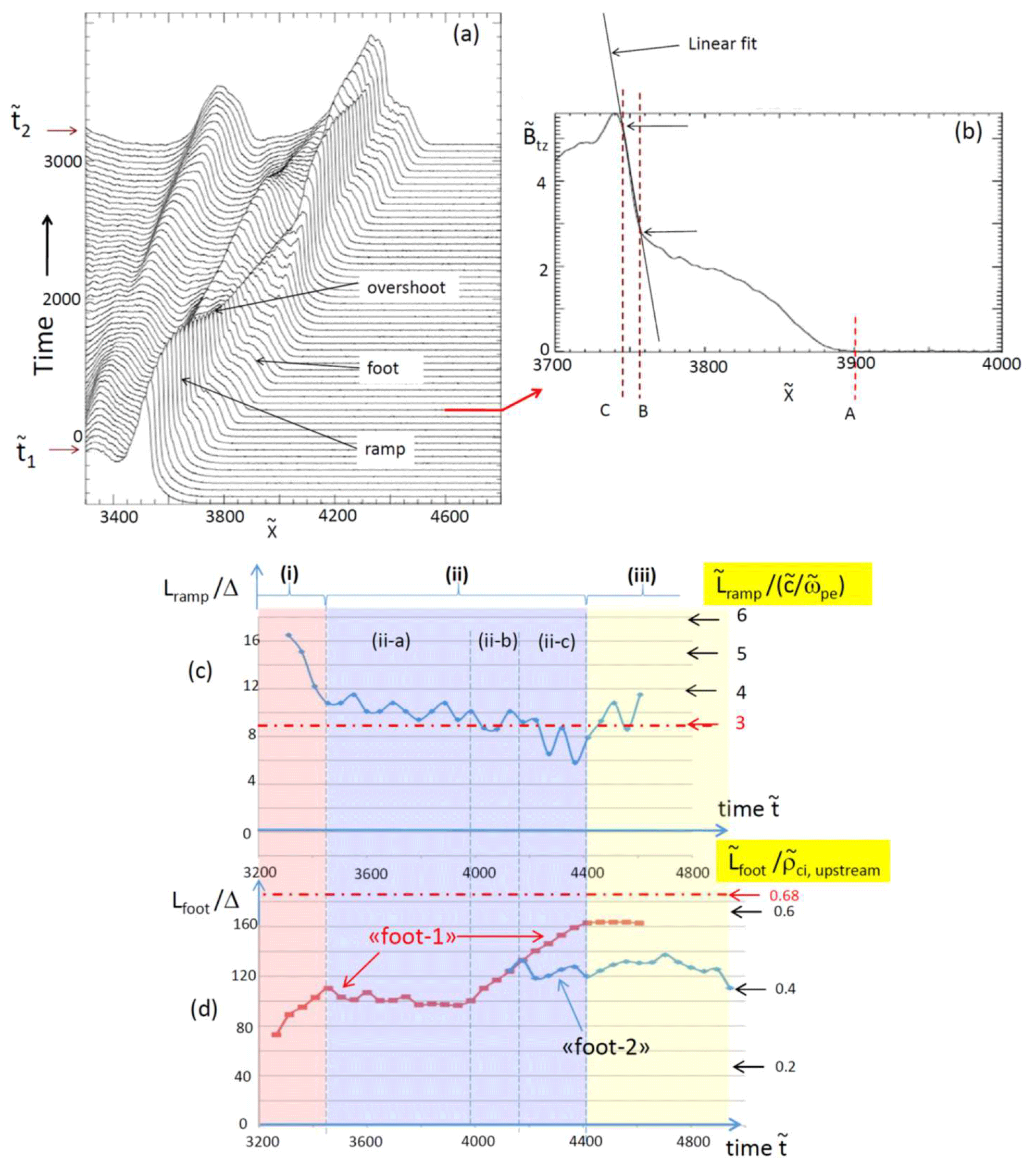
Figure 11 (a) Time stack plot of the main magnetic field component ${\stackrel{\mathrm{̃}}{B}}_{tz}$ versus axis $\stackrel{\mathrm{̃}}{x}$ (the time evolves from the bottom to the top curve, and the propagation of the shock front is along the $\stackrel{\mathrm{̃}}{x}$ axis from the left to the right-hand side). Results are issued from 2D PIC simulation (where the B₀ static field is out of the simulation plane $\stackrel{\mathrm{̃}}{x}-\stackrel{\mathrm{̃}}{y}$); the ${\stackrel{\mathrm{̃}}{B}}_{tz}$ profile has been space averaged along $\stackrel{\mathrm{̃}}{y}$ axis; the temporal interval between two successive curves is $\mathrm{\Delta }\stackrel{\mathrm{̃}}{t}=\mathrm{48}$, and the time stack plot covers the time interval $\mathrm{3456}<\stackrel{\mathrm{̃}}{t}<\mathrm{6048}$; (b) blown-up view of the spatial profile of the main magnetic field component ${\stackrel{\mathrm{̃}}{B}}_{tz}$ defined at a fixed time ($\stackrel{\mathrm{̃}}{t}=\mathrm{4128}$) indicated by the red arrow in (a); the locations of the bounds A, B, and C are illustrated by vertical dashed lines. Time history (c) of the ramp thickness measured within the range BC (defined in b) normalized versus the upstream electron inertial length $c/{\mathit{\omega }}_{\mathrm{pe}}$ (right-hand side scale) and (d) the foot thickness measured within the range AB (defined in b) normalized versus the upstream ion gyroradius ρ_ci (right-hand side scale), during a cyclic self-reformation period (${\stackrel{\mathrm{̃}}{\mathit{\tau }}}_{\mathrm{ref}}=\mathrm{1523}$). In (c) and (d), the spatial widths are normalized versus the unit space grid Δ on the left-hand side scale. The respective lower- and upper-bound values of the ramp and the foot thickness are reported by dashed–dotted red horizontal lines in (c) and (d), respectively. Note that the width of ramp-1 is only represented in (c) in order to avoid overwhelming the plot; the small time fluctuations in ramp-1 correspond to error bars of the measurements (which are based on y-averaged ${\stackrel{\mathrm{̃}}{B}}_{tz}$ profiles).

The variation of the ramp width versus time reported in Fig. 11c shows that three successive time ranges can be defined where, respectively, the width decreases (range i defined by $\stackrel{\mathrm{̃}}{t}<\mathrm{3456}$), very slightly decreases (range ii defined by $\mathrm{3456}<\stackrel{\mathrm{̃}}{t}<\mathrm{4400}$), and increases (range iii defined by $\stackrel{\mathrm{̃}}{t}>\mathrm{4400}$) as represented by pink, blue, and yellow areas, respectively. Then, the width stays almost constant during a large time range (ii). Within this range, the width reaches a lower-bound value around $\mathrm{3}c/{\mathit{\omega }}_{\mathrm{pe}}$ (dashed–dotted red line), which can be used as a reference scale in the comparison with experimental data instead of comparing exact scales measured at a given crossing time of the shock. In order to analyze the whole-time variation of the ramp width in detail, it can be associated with that of the foot and with ion phase space as described in Sect. 4.4.2.

4.4.2 Results on the foot thickness

Figure 11d shows the time variation of the foot width issued from the same PIC simulation. The upstream edge of the foot (vertical dashed line A in Fig. 11b) is defined as the location where the magnetic field has increased by 6.67 % over its upstream value (Burgess et al., 1999; Yang et al., 2009, 2011). The value of 6.67 % has been determined as corresponding to the maximum amplitude in the magnetic field fluctuations measured upstream (which is sensitive to the particle number per cell). Then, the amplitude of the upstream magnetic field turbulence is below the value (1 + 6.67 %) ×B₀ in our simulations.

The time variation of the foot width can be detailed with the help of the three time intervals defined for the ramp thickness in Sect. 4.4.1 and is associated with the ramp as follows. In range (i), the foot width increases in anticorrelation with the ramp variation; at that time, reflected ions are accelerated at the ramp and only initialize their gyromotion (not shown herein). The range (ii) (where the ramp width slightly decreases) includes three successive phases for the foot dynamics: one (ii-a) where the foot width is constant ($\mathrm{3456}<\stackrel{\mathrm{̃}}{t}<\mathrm{3984}$), another (ii-b) where the foot width strongly increases ($\mathrm{3984}<\stackrel{\mathrm{̃}}{t}<\mathrm{4176}$), and a last one (ii-c) where the foot width is still increasing. But, in addition, a secondary foot can be identified upstream (blue curve for $\stackrel{\mathrm{̃}}{t}>\mathrm{4176}$); a double foot appears as detailed below. Finally, in range (iii) ($\stackrel{\mathrm{̃}}{t}>\mathrm{4416}$), the foot width reaches a maximum value ($L_{\mathrm{foot}}/{\mathit{\rho }}_{\mathrm{ci},\mathrm{us}}$) = 0.6, which remains constant at later times while the ramp thickness starts increasing.

A detailed analysis of the ion phase space (not shown here) at these corresponding time intervals allows us to interpret more precisely the time variation of both ramp and foot thicknesses. In range (i) (i.e., $\stackrel{\mathrm{̃}}{t}<\mathrm{3456}$), the ramp (named ramp-1) is freshly formed from the steepening of the foot resulting from the previous self-reformation and the foot in panel (d) is only due to the old reflected ions (previous self-reformation) still located upstream of the new ramp-1 while accomplishing their full gyration (before being transmitted downstream); this steepening corresponds to the decrease of the ramp width (range i in panel c). In range (ii-a), ramp-1 starts to accelerate and reflect new upstream ions, which add to old reflected ions which did not reach the downstream region yet. Then, the local foot (named foot-1) is composed of two (old and new) reflected ion populations (reflected at two successive reformation cycles). During this acceleration phase, the energy of macroscopic fields at the ramp is transferred to newly reflected ions, which smooths the local steepening, and the ramp-1 width slightly decreases only. Within the range (ii-b), all old reflected ions have reached the downstream region; only freshly reflected ions are present upstream of the ramp, continue their gyromotion, and contribute to foot-1. Consequently, the foot-1 width strongly increases as mainly carried by these newly reflected ions. Correspondingly, the width of ramp-1 still slightly decreases. But, more and more new ions are reflected and accumulate in time, and a local new foot (named foot-2 ) builds up. This ion accumulation is large enough so that the upstream edge of this new foot-2 steepens and becomes a new ramp (named ramp-2, not shown in panel d) which starts reflecting new ions; let us mention that the width of ramp-2 cannot be precisely identified before $\stackrel{\mathrm{̃}}{t}<\mathrm{4368}$ by using the best linear fit (as in Fig. 11b) since this part of the front microstructure is still mainly dominated by the growing foot (steepening is not strong enough in the upstream edge of foot-2 within this time range). This new foot-2 (blue curve in panel d) co-exists with the old foot-1 (red curve) within the same time interval $\stackrel{\mathrm{̃}}{t}>\mathrm{4176}$. Simultaneously, the amplitude of the new overshoot (not shown here) associated with the new ramp-2 increases, and the field gradient between the old and the new overshoot becomes weaker. Therefore, the ramp-1 width increases at a later time (time range iii). For $\stackrel{\mathrm{̃}}{t}>\mathrm{4608}$, the old ramp-1 is totally absorbed into the shock profile (between the old and the new overshoots), and its width cannot be identified precisely.

Then, the shock front may acquire a multi-peak profile including traces of old and new successive ramps (not to be confused with emission of large amplitude whistler waves emitted from the main ramp). The width of the whole shock front is the summation of the ramp and the feet contribution and can be estimated from the upper edge of the new foot-2 to the lower edge of the old ramp in the front. Present results provide maximum value measured at the final stage of self-reformation cycle (${\stackrel{\mathrm{̃}}{L}}_{\mathrm{shock},\max }=\mathrm{176.3}=\mathrm{2.93}\stackrel{\mathrm{̃}}{c}/{\stackrel{\mathrm{̃}}{\mathit{\omega }}}_{\mathrm{pi}}$ at $\stackrel{\mathrm{̃}}{t}=\mathrm{4608}$). Let us stress that this value represents an upper bound of the shock front width and not a common measurement of the front width itself.

5 Comparison with some previous studies

This section is dedicated to comparing the present results with those issued from previous studies. The main emphasis is given not only on the agreement or disagreement observed between the different results but also – and even more importantly – on the strategy used in previous studies for “extracting” the spatial width of the shock front microstructures. We will distinguish previous studies dedicated to measurements of the ramp and of the foot thicknesses.

5.1 Spatial measurements of the ramp thickness

5.1.1 Newbury and Russell (1996)

Most studies based on the analysis of experimental data issued from ISEE-1 and ISEE-2 satellites indicate a scaling of the ramp width within the ion inertial length. In a very detailed analysis of a single shock crossing, Scudder et al. (1986) have reported the ramp thickness to be $\mathrm{0.2}c/{\mathit{\omega }}_{\mathrm{pi}}$, a measurement which was based on an exponential fit of the foot–ramp transition. By using the same fit technique, Russell and Greenstadt (1979) have measured a slightly thicker ramp of about $\mathrm{0.4}c/{\mathit{\omega }}_{\mathrm{pi}}$ in an initial study of ISEE bow shock observations. Later on, Newbury and Russell (1996) analyzed seven nearly perpendicular shocks (${\mathit{\theta }}_{B_n}>\mathrm{80}$^∘) and found a range of ramp widths (based on a linear fit to the ramp transition) from 0.5–0.8 $c/{\mathit{\omega }}_{\mathrm{pi}}$. However, in one case the ramp width was particularly thin $\mathrm{0.05}c/{\mathit{\omega }}_{\mathrm{pi}}$ (= $\mathrm{2}c/{\mathit{\omega }}_{\mathrm{pe}}$). To the knowledge of the authors, it was the first time that such a thin ramp had been observed associated with the terrestrial shock. All the observations lead to the following statements:

• a.

  In contrast with the tentative explanations proposed at that time (summarized in Newbury et al., 1998), this very thin ramp ($\mathrm{2}c/{\mathit{\omega }}_{\mathrm{pe}}$) takes a full meaning herein and is in quite good agreement with the present statistical results. It represents quite well a potential signature of the self-reformation process which allows the ramp to have a very small thickness (a few $c/{\mathit{\omega }}_{\mathrm{pe}}$).

• b.

  One question arises. Why do most previous studies show mainly a ramp width scaling with a noticeable part of the ion inertial length (except the very narrow ramp mentioned above), which is in contrast to the present results? Several answers can be proposed. First, the method commonly used in previous studies and based on exponential fitting to the foot–ramp region is not appropriate to measure carefully the ramp and foot thickness, respectively, since both fine structures were mixed together. This fitting methodology is a source of important errors. Second, the solar wind conditions corresponding to the set of shock crossings chosen at that time need to be verified carefully. Indeed, as β_i is relatively low (β_i=0.17 as in Hada et al. (2003), or equivalently $v_{\mathrm{sh}}/v_{\mathrm{thi}}$ equals several decades as in Scholer et al., 2003), the reflected ions describe a focused (narrow) beam during their gyration. These maintain a well coherent gyromotion which forces them to accumulate at a certain distance from the ramp and to initialize the foot. The growth of the foot separates clearly from the ramp and is characterized by a trapping loop in the ion phase space; self reformation takes place, and the front is nonstationary.

In contrast, as β_i is relatively high (β_i=0.35 as in Hada et al., 2003, or $v_{\mathrm{sh}}/v_{\mathrm{thi}}$ equals a few units as in Scholer et al., 2003), the reflected ions rapidly diffuse as they start their gyromotion; these lose their large coherent motion and spread out within the whole front (no clear ion trapping loop). The foot grows up but does not separate from the ramp. Then, ramp and foot are mixed, and a larger thickness of the ramp–foot region is expected as shown in PIC simulations of Lembège et al. (2013a, b). Then, no self-reformation can take place, and the shock front is stationary.

5.1.2 Newbury et al. (1998)

At the ISEE-1 and ISEE-2 time, the ramp was usually characterized by two different scales: (i) a large scale (or global ramp width) within which the main transition from upstream to downstream magnetic fields takes place and (ii) a thinner subramp scale which contains steep jumps in the magnetic field with amplitudes sometimes comparable to the overall change in the magnetic field at the shock. One conclusion (Newbury et al., 1998) was that both scales are characteristic of the quasi-stationary shock profile (which – at that time – was considered stationary within the ion gyroperiod). More precisely, Newbury et al. (1998) have analyzed a set of 20 shock crossings and found that the width of the overall ramp transition is typically within the range 0.5–1.5 $c/{\mathit{\omega }}_{\mathrm{pi}}$, which is quite large as compared with our present measurements. This difference can be easily explained by the fact that the authors have defined the ramp thickness based on a linear fit of the total magnetic field profile from the foot to the overshoot, which enlarges the estimate of the ramp thickness, as compared with the present method used in Sects. 3 and 4.

Cluster data and present statistical results allow us to correct this view within the frame of the intrinsic shock front self-reformation. The so-called “large scale” of the ramp presents a large width variability (extending from a part of the ion inertia length to a few electron inertia lengths as displayed in Fig. 9a), which was not observed at that time for the reason mentioned above. But, simultaneously, the so-called “small scales” can result from instability developing with the foot region as the ECDI, which represents Electron Cyclotron Drift Instability (Muschietti and Lembège, 2006, 2013) or MTSI (Scholer et al., 2003; Matsukyio and Scholer, 2003; Muschietti and Lembège, 2017), for instance, and can propagate (convection effects). In the present work, the use of a linear fit applied within the ramp region only (as described in Sect. 3) allows us to average these local small-scale fluctuations and to measure the ramp width with minimizing errors. Analyzing small-scale field fluctuations (as those also observed within the ramp in Figs. 3 and 5) requires a further investigation which will be presented elsewhere.

5.1.3 Bale et al. (2003)

From the spacecraft floating potential measured on board the four Cluster satellites, Bale et al. (2003) have determined the electron plasma density and studied the macroscopic density transition scale at 98 crossings of the quasi-perpendicular terrestrial bow shock. This first tentative clue for measuring the shock transition width from Cluster data was attractive but contains several limitations for the following reason: a hyperbolic tangent function has been fitted to each density transition in order to capture the main shock transition but no microstructures of the front – as foot, ramp, or overshoot – have been identified and scaled. Such a fit partially includes parts of the shock front outside the ramp itself so that it cannot apply to determine the ramp thickness with acceptable accuracy since both ramp and foot structures are not separated. This technique takes into account only the widest transition scale at the shock front, which overestimates the ramp width and restricts drastically its application. Then, the conclusions stating that, for high Mach number shocks (including the range M_A = 4–5 as that considered in the present work), only the convected gyroradius is the preferred scale for the shock density transition are strongly questionable since the real ramp is much thinner. This resulting scale corresponds to the scale of the foot rather than that of the ramp, and no conclusive statements can be obtained.

On the other hand, in the light of Cluster data, looking for an estimate of the shock transition presents, nowadays, a limited interest, since recent results show that terrestrial shock is rather nonstationary and a “unique” typical spatial scaling must be replaced by some interval or bounds of variation (lower bound and upper bound) within which the spatial scales of the fine structures can vary.

Figure 12 helps us to better compare our results with those by Bale et al. (2003), which have been reproduced in Fig. 12a, b, and d. The same representation as in Fig. 12b and d has been used for Fig. 12c and e to plot the front thickness computed as the sum of the ramp and the foot thicknesses from our methodology versus the magnetosonic Mach number M_ms. The pink area in Fig. 12b illustrates the range of M_ms explored from the present study. Figure 12c reveals that in this range of M_ms values no clear dependence considering the large error bars (as on above Fig. 12b) can be identified from the present study. It would be obviously impossible here to conclude that the front thickness simply increases with M_ms and conversely the best fit would conclude here that there is a trend to decrease. Our results are therefore in strong contradiction with conclusions of Bale et al. (2003). Moreover, if we consider another M_ms range of similar extension as the one shown in Fig. 12c from our study and highlighted by the green area in Fig. 12b, a similar representation (not shown here) would conclude to exactly the opposite to what the dotted line in Fig. 12b shows, considering again the large error bars. This illustrates again the impossibility to make a simple scaling of the front thickness by a single parameter as the magnetosonic Mach number. Figure 12e shows that the front thickness normalized by the downstream gyroradius is more or less consistent with the results of Bale et al. (2003) shown in Fig. 12d. There is a trend there to decrease with M_ms increase. As mentioned in the present study, the use of the so-called “density transition scale” by Bale et al. (2003) shown in Fig. 12a is inappropriate since it mixes the time variability of the ramp and the ion foot. They also mention a stationary shock from their Fig. 1. But, this figure does not show the highest temporal resolution of the magnetic field data but only corresponds to five values per second. For many shock crossings used in the present study, the profiles displayed at 5 Hz look very similar, whereas the highest-time-resolution profiles clearly reveal different features (as illustrated in our Fig. 6).

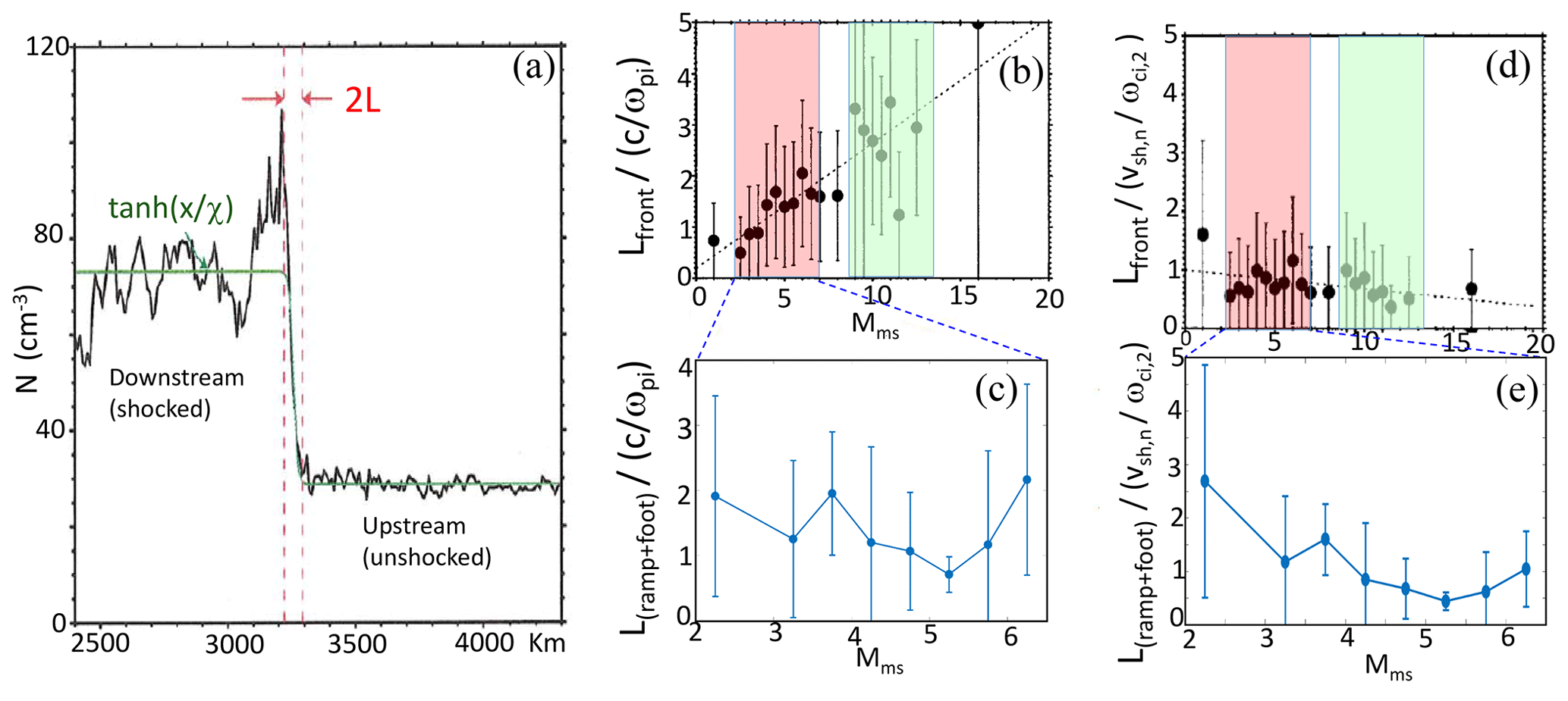
Figure 12 Panels (a), (b), and (d) are issued from Figs. 3 and 6 of Bale et al. (2003) for the shock crossing on 15 December 2000 at 01:26:15, while (c) and (e) are similar to (b) and (d) but correspond to results from the present analysis. Panel (c) has to be compared with an enlarged view of (b) within the magnetosonic Mach number range $\mathrm{2}<M_{\mathrm{ms}}<\mathrm{6.5}$. Panel (a) shows the transition of the density from upstream (unshocked) to downstream (shocked) states for a magnetosonic Mach number M_ms=3.5 and ${\mathit{\theta }}_{B_n}=\mathrm{81}$^∘ shock (see text), where $M_{\mathrm{ms}}=V_{\mathrm{sw},\mathrm{sc}}/c_{\mathrm{ms}}$ with $c_{\mathrm{ms}}=(c_{\mathrm{s}}^{\mathrm{2}}+v_{\mathrm{A}}^{\mathrm{2}}{)}^{\mathrm{1}/\mathrm{2}}$, c_s is the sound speed, and V_sw,sc is the bulk velocity of solar wind measured in the frame of the spacecraft; the green line is the hyperbolic tangent fit, and red vertical lines show the density transition scale. In panels (b) and (d), pink and green areas are superimposed on results by Bale et al. (2003) to indicate, respectively, the same M_ms range as for our study and another M_ms range (same width) for higher values for comparison. Panel (c) issued from the present results shows the variation of the shock front thickness L_(ramp+foot) versus the M_ms range corresponding to the pink area defined in (b) where L is normalized to the ion inertial length $c/{\mathit{\omega }}_{\mathrm{pi}}$ defined upstream. Panel (e) issued from the present results shows the variation of the shock front thickness L_(ramp+foot) versus M_ms for the same range, where L is normalized to ($v_{\mathrm{sh},\mathrm{n}}/{\mathrm{\Omega }}_{\mathrm{ci},\mathrm{2}}$) in order to compare with panel (d), where v_sh,n is the shock normal velocity defined in the frame of the solar wind, and Ω_ci,2 is the proton gyrofrequency defined downstream.

5.1.4 Krasnoselskikh et al. (2002)

Krasnoselskikh et al. (2002) have proposed another mechanism as a possible source of nonstationarity of the shock front (so-called gradient catastrophe), where the shock appears as a balance between nonlinear and dispersive effects only. In this mechanism, the transition to nonstationarity is characterized by the lack of the phase standing whistler wave train inside the shock front. This process takes place for oblique quasi-perpendicular shock (for a direction ${\mathit{\theta }}_{B_n}$ not too far from 90^∘) as the Alfvén Mach M_A is above a certain critical Mach number given by $M_{\mathrm{nw}}=(\mathrm{1}/\mathrm{2}{)}^{\mathrm{1}/\mathrm{2}}(M_{\mathrm{i}}/m_{\mathrm{e}}{)}^{\mathrm{1}/\mathrm{2}}\cos {\mathit{\theta }}_{B_n}$; this condition can be equivalently expressed for a fixed M_A as the direction ${\mathit{\theta }}_{B_n}$ is below a critical angular value. In this case, the nonlinear steepening of the wave train cannot be balanced by the dispersion effects alone. However, as mentioned in Sect. 1, this theoretical mechanism has severe limitations since (i) it is based on a 1D model only and (ii) it excludes any dissipative effect. Indeed, reflected ions (which play a key role in supercritical Mach regime) are neglected, and their impact on the shock dynamics – and in particular on the temporal fluctuations of the shock front microstructures which is our center of interest in the present paper – is totally absent. Because of the above severe limitations, this process is still a source of controversy and is not considered herein.

5.1.5 Lobzin et al. (2007)

Nevertheless, a further study made by Lobzin et al. (2007) has proposed the gradient catastrophe process as being at the origin of the shock front nonstationarity observed by Cluster on 24 January 2001. While the front nonstationarity is quite clear in the experimental data which show quite different shock front profiles of the magnetic field crossed by the four satellites of Cluster, the proposed interpretation stays quite questionable for the following reasons: (i) the overall analysis is based on one shock crossing only (no statistical analysis has been performed), (ii) no procedure detailing the transfer from time to spatial scaling of the shock front (in particular focused separately on the ramp or foot structures) has been indicated, so one ignores the percentages of errors underlying the spatial field profiles measurements which are not shown; (iii) no mapping and/or basic information have been provided on the 3D disposal and inter-distance of the satellites, so one ignores whether the four satellites cross the same shock front within the same or different successive self-reformation cycles; (iv) only one measurement of the ion density showing some fluctuations has been presented which is not enough for confirming that it could be due to the gradient catastrophe process. Moreover, note that such similar density fluctuations have been also measured quantitatively versus time in previous numerical simulations (Lembège and Savoini, 1992; Yang et al., 2009) but have been attributed as being due to the self-reformation process fed by the accumulation of reflected ions and not to the gradient catastrophe process. Similar self-reformations have been also obtained as supported by the MTSI for an obliquely propagating shock (Comisel et al., 2011); (v) a deeper analysis shows that the upstream ion temperature used in this paper is not the correct one since the CIS instrument was in magnetospheric mode (see Sect. 2), so the moment calculations provide a large overestimate of the solar wind proton core temperature. Indeed, the determination of the upstream ion thermal velocity requires a delicate procedure and is of central interest since the stationarity or nonstationarity of the shock front is strongly dependent on the ratio $v_{\mathrm{sh}}/v_{\mathrm{thi}}$ (Scholer et al., 2003) or similarly on the ratio β_i (defined as the ion kinetic energy over magnetic energy) (Hada et al., 2003). When using the solar proton temperature from the ACE satellite (4.5 eV thermal energy), the ion beta found is 0.6 instead of the value of 2.0 reported by Lobzin et al. (2007).

5.1.6 Comisel et al. (2011)

The same data of Cluster measured on 24 January 2001 has been re-examined in detail by Comisel et al. (2011) and re-interpreted quite differently by using PIC simulations in plasma conditions and Mach number regimes chosen to be appropriate with experimental conditions. Basically, the authors have shown that the self-reformation is quite well recovered but is not controlled by the gradient catastrophe process (dispersive effects only) mentioned above but rather by the self-reformation mechanism fed up by the MTSI which is an indirect consequence of the ion reflection (dissipative effects which have been neglected in Krasnoselskikh et al., 2002). Indeed, for slightly oblique shocks (out of 90^∘), the MTSI develops between the incoming electrons and incoming ions, with a growth rate large enough to develop during the gyration of the reflected ions (Scholer and Matsukiyo, 2004). These authors have shown that for a nonrealistic mass ratio, the self-reformation is still controlled by the collection of reflected ions at the upstream edge of the foot as in Lembège and Savoini (1992), since the MTSI has a weak growth rate and has no impact on the nonstationary dynamics of the shock front. In contrast, for realistic mass ratio, the growth rate is much larger, and MTSI can be easily excited, which leads to ion phase mixing and thermalization. Then, the ion pressure increases considerably locally somewhere within the foot itself (and not at the edge of the foot) with associated building up and overtaking of the magnetic field. A new shock ramp builds up within the foot which initiates to reflect new incoming ions and a cyclic reformation is initialized. The cyclic period is lower than the one associated with the self-reformation due to the accumulation of reflected ions (as in Lembège et Savoini, 1992), since the process takes place before ions accomplish their full gyration. More precisely, by using the appropriate conditions of the 24 January 2001 shock crossing in the PIC simulations, Comisel et al. (2011) have shown that the waves triggered by this instability are of whistler type and have phase velocities directed downstream in the shock frame, and the associated Poynting flux (and wave group velocity) is also directed in the downstream direction. However, as these approach the density and magnetic field overshoot, the waves are refracted; as a consequence, the Poynting flux changes direction and is directed upstream in the shock frame. In summary, there is no indication of a phase standing linear or nonlinear whistler precursor produced by the shock ramp itself in this process. This scenario does not support the scenario that proposed by Krasnoselskikh et al. (2002), where a nonlinear whistler precursor is required to initialize the gradient catastrophe process as a source of the front nonstationarity.

5.1.7 Hobara et al. (2010)

A statistical study based on 77 crossings of the terrestrial bow shock (30 by THEMIS (Time History of Events and Macroscale Interactions during Substorms) and 47 by Cluster) has been performed by Hobara et al. (2010) in order to analyze the ramp scale and the associated gradient width. Their study claims that the spatial scale of the ramp decreases as the shock Alfvén Mach number increases. However, detailed comparison with our results is difficult (almost impossible) at the present time because of important missing information. (i) No detailed information is provided on the procedure used for extracting the spatial widths of the ramp from the temporal experimental data as detailed in present Sect. 2; (ii) the duration of the ramp crossing has been defined as a time interval between the upstream edge of the ramp and the maximum of overshoot. However, let us note that the upstream edge is not defined precisely (see the precaution to account for in our Sect. 3), and the use of the overshoot can lead to an overestimate of the ramp width as compared to the method used herein (Sect. 3) since it is partially polluted by reflected ions; (iii) statistical errors are indicated in their Figs. 2 and 3 only for a range of Mach numbers and not on individual measurements; (iv) no statistics are shown versus the direction (${\mathit{\theta }}_{B_n}$) of the shock front normal; as a consequence, one ignores how and whether the measurements of the ramp or foot bounds are polluted by the whistler (either linear or nonlinear), whose emission strongly depends on the angle ${\mathit{\theta }}_{B_n}$; (v) no statistics or information is indicated on the ion β_i value (which has a strong impact on the shock front self-reformation) (Hada et al., 2003); (vi) the authors use two different statistics: one based on the ramp spatial scale (their Fig. 3) and the other based on magnetic ramp spatial gradient scale (their Fig. 4). Moreover, they used a simple theoretical argument (based on dispersive whistler) to stress that the wavelength L_w of the linear or nonlinear whistler varies as $L_{\mathrm{w}}\sim \mathrm{1}/M_{\mathrm{A}}$. But the fact that both statistics show that the width of the measured structure decreases as M_A increases does not imply that dispersion determines the size of the magnetic ramp even for supercritical shocks (as discussed later on); (vii) at least, only a very limited number of measurements (whatever the M_A value is within the concerned range M_A = 2–12 in Hobara et al., 2010) indicate that the ramp width succeeds to reach a few electron inertial lengths (equal to or lower than $\mathrm{5}\stackrel{\mathrm{̃}}{c}/{\stackrel{\mathrm{̃}}{\mathit{\omega }}}_{\mathrm{pe}}$, in their Figs. 2 and 3), which is in strong contrast with our statistical results of Fig. 9a. The lack of statistics versus ${\mathit{\theta }}_{B_n}$ and β_i (above points iv and v) and the absence of precise information on the methodology used in the statistics of Hobara et al. (2010) (as listed above) could explain this difference.

Moreover, Hobara et al. (2010) deduce that their measurements (in particular the decrease of the ramp thickness as M_A increases) show that the major process responsible for the shock front nonstationarity is the gradient catastrophe process proposed by Krassnoselskikh et al. (2002) and Lobzin et al. (2007). However, three main facts contradict this statement: (i) the first is arguments describing the severe limitations of the theoretical model (Krassnoselskikh et al., 2002) and the revised analysis of Comisel et al. (2011) as already described above in the present section, (ii) Hobara et al. (2010) use the overshoot (observed in the set of their experimental measurements) as an upper bound to define the ramp width, but the overshoot of supercritical shocks is a clear signature of the reflected ions as these gyrate downstream after being once reflected at the ramp (Leroy et al., 1982). Then, a contradiction occurs since dissipation effects (strongly carried by the reflected ions) have been fully neglected in the model of gradient catastrophe which cannot support their statements; (iii) a similar variation of the ramp thickness as M_A increases has also been observed in the self-reformation process in PIC simulations (not shown here), which means that this variation cannot be used as a unique signature of the gradient catastrophe process. At least, in order to support their statements, Hobara et al. (2010) recall that PIC simulations evidencing the self-reformation due to the accumulation of reflected ions at a foot distance from the ramp (as in Lembège and Savoini, 1992) as well as due to the MTSI (as in Matsukyio and Scholer, 2006 use low ${\mathit{\omega }}_{\mathrm{pe}}/{\mathit{\omega }}_{\mathrm{ce}}$ ratio, which overestimates the electric field to magnetic field ratio (in practice, using a realistic ${\mathit{\omega }}_{\mathrm{pe}}/{\mathit{\omega }}_{\mathrm{ce}}$ ratio is very difficult at present time for computational constraints). If were true, this argument would suggest that the electric field would be too large and that the self-reformation process would result from an artifact. However, no quantitative result has been obtained until now to support such a statement. In contrast, let us remind the reader that (i) the parametric analysis performed by Lembège et al. (2009) clearly shows that both hybrid and PIC simulation retrieve the same self-reformation process of the shock front in similar plasma conditions and Mach regime, provided that the space grid is small enough (i.e., high resolution) in hybrid simulations as shown initially by Hellinger et al. (2002); this last result would suggest that the field gradients at the ramp are important and not the absolute fields amplitude; (ii) electron scales are neglected in common hybrid simulations (as those used in Hellinger et al., 2007; Lembège et al., 2009, and references therein), which are independent of the ratio ${\mathit{\omega }}_{\mathrm{pe}}/{\mathit{\omega }}_{\mathrm{ce}}$. This suggests that the ratio ${\mathit{\omega }}_{\mathrm{pe}}/{\mathit{\omega }}_{\mathrm{ce}}$ has no direct impact on the self-reformation. Note that the ramp width may be estimated in terms of percentages of ion inertial length in hybrid simulations and both in terms of electron and ion inertial lengths in PIC simulations.

In summary, the measurements of Hobara et al. (2010) do not support the model describing the ramp as an evolving nonlinear whistler wave; neither does the mechanism of the gradient catastrophe process of Krassnoselskikh et al. (2002) as a source of the front nonstationarity.

5.1.8 Schwartz et al. (2011)

Schwartz et al. (2011) have determined the scale of the electron temperature gradient via electron distributions measured in situ by the Cluster spacecraft and have identified two different scales: when the Mach number is supercritical (M_A=3.8) and when the shock propagation is oblique (${\mathit{\theta }}_{B_n}=\mathrm{83}$^∘). First, the authors found that half of the electron heating coincides with a narrow layer covering several electron inertia lengths ($c/{\mathit{\omega }}_{\mathrm{pe}}$) and found an inflated electron distribution due to primarily the electron filling in or the entrapment in regions of phase space that would not be accessible. Second, the remaining solar wind maximum is only present in the smoother increase of the field which precedes the ramp; this beam is totally destroyed by the time this electron scale ramp is crossed. The authors found that this scale is comparable to that deduced from the theoretical limiting case of a wave capable of phase standing in the incident flow and concluded that this suggests that supercritical shocks steepen to this whistler limit since dissipation processes are insufficient to broaden the transition further.

However, several elements of information are missing: (i) the authors mentioned to have used a technique to convert the time series of data to distance along the shock normal similar to that of Schwartz (1998), i.e., the procedure to determine the normal and the velocity of the shock from multi-spacecraft measurements (as in Sect. 2), but did not provide detailed information on the procedure itself, associated errors estimate, or on the definition of the ramp itself (their Fig. 1); (ii) the results are limited to one shock crossing (one spacecraft only), and some attempts for other shock crossings are mentioned, but no statistical results have been shown or summarized; (iii) the observed results cannot lead to the conclusions that dissipation processes are insufficient to broaden the transition further, since once again the key dissipation processes driven by the (reflected) ions are not mentioned or analyzed in the study. Of course, dispersive effects must be considered in the global balance of nonlinear steepening of the front by both dispersive or dissipative effects, but this does not mean that the shock front dynamics are controlled by dispersive effects. Moreover, other sources of field fluctuations may take place in the shock front (such as formation of multi-peaks (signatures of old or new self-reformation (Sect. 4.4.2) and/or whistler waves excited by the MTSI within the front) without invoking any dispersive effect.

5.1.9 Yang et al. (2020)

Very recently, Yang et al. (2020) claimed to have identified shock front self-reformation with the help of high-resolution Magnetospheric MultiScale (MMS) satellite data. This study using measured ion phase space together with B profiles clearly shows the importance of dissipation effects carried by the reflected ions. However, the comparison with the results of the present study proves to be quite difficult due to the lack of precise information. While the MMS data show clearly that the crossed shock is nonstationary, a clear proof of the self-reformation is still questionable for the following reasons:

• a.

  The whole study is based on one shock crossing only and eventually restricted to a comparison between two satellites since three of them show very similar profiles and appeared to be in a plane nearly parallel to the shock front. No statistical results are shown or even summarized, which could have stressed the ion vortex formation over different steps of its formation.

• b.

  The authors mentioned to have used the timing technique (Schwartz, 1998) to determine the normal and the velocity of the shock front from multi-spacecraft measurements. But no information is given on the application of the procedure itself (in each spacecraft frame) or on the estimate of associated errors. The use of typical magnetic field peaks around the overshoot is mentioned but without specifying where in the different time series. The use of the overshoot is quite odd since it is not precise enough (contrary to the middle of the ramp) as a reference point; indeed, it contains superimposed fluctuations and is partially polluted by reflected ions. Moreover, important information equivalent to reference satellite and reference time (as proposed in our Sect. 2.2) are missing. In addition, no information is given on the identification of the ramp itself and on the conversion from the time series to distance profile along the shock normal.

• c.

  The analysis mentions a shock ramp of less than 0.3 $c/{\mathit{\omega }}_{\mathrm{pi}}$, which is not precise enough, seems high, and is in contrast with the fact that M_A is relatively high (M_A=10.8). For such a value, one could expect a much narrower ramp width (see statistics in our Fig. 9d). In addition, one ignores (i) how this ramp width has been measured and (ii) the precise values of the ramp width during the shock crossing by each satellite.

• d.

  The emerging large-scale fluctuations announced as a new ramp for only one satellite may be questionable. The new front is not “mature” enough during the shock crossing, and the precise location of the “new ramp” within these fluctuations is not clearly identified. One can wonder whether it could be the signature of front rippling and/or multi-crossing due to the back and fourth motion of the shock front, which would need a further analysis.

5.2 Spatial measurements of the microstructures

Walker et al. (2004) investigated short-scale structures in the electric field that are observed during crossings of the quasi-perpendicular bow shock using also data from the Cluster satellites. An example is reproduced from this paper in Fig. 13a. The structures observed at each Cluster satellite exhibit large amplitudes, as high as 70 mV/m, and the authors argue that they make a significant contribution to the overall change in the potential at the shock front. They have shown that the scale size of these short-lived electric field structures is on the order of a few $c/{\mathit{\omega }}_{\mathrm{pe}}$ as shown in their statistics reproduced in Fig. 13c. They also studied the relationships between the scale size and the upstream Mach number and ${\mathit{\theta }}_{B_n}$. They found that the scale size of these structures decreases with decreasing β_i and as ${\mathit{\theta }}_{B_n}$ approaches 90^∘.

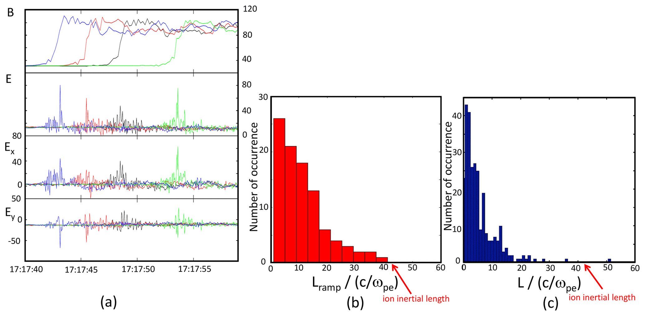
Figure 13 Panels (a) and (c) are reproduced from Walker et al. (2004). Panel (a) displays an example of short-scale electric field structures observed around the crossing of the bow shock by the Cluster quartet on 31 March 2001 at 17:18 UT (first panel: spin time-resolution magnetic field magnitude; the following panels display the amplitude of the electric field and E_x and E_y GSE components, respectively). Panel (b) reproduces the distribution of magnetic field ramp obtained from the present study already shown in Fig. 9a to compare with the distribution of the electric field structures of Walker et al. (2004) shown in (c).

Interestingly, the comparison of distributions displayed in Fig. 13b (present analysis) and Fig. 13c (Walker et al., 2004) shows that the electric field structures are consistent with microstructures of the ramp since the typical scales found seem smaller. Of course, to be fully conclusive, one would need to compare the size of the electric field structure and of the magnetic ramp for each shock crossing. However, both results seem very consistent. Recently, Dimmock et al. (2019) have shown electron-scale field structures inside the shock ramp from a case study using the observations of only two Cluster spacecraft which were very close to each other, and they proposed that it is associated with the transition to nonstationarity.

5.3 Spatial measurements of the foot thickness

As compared with studies focused on the ramp width, previous studies dedicated to the spatial measurements of the foot thickness are in relatively limited number. First observations of the foot have been made by Paul et al. (1965). Woods (1969, 1971) has proposed the reflected ions to account for the foot structure and has estimated a foot width for a strictly perpendicular shock from the turning point distance (Eq. 4 of Sect. 4.3, which is recalled here):

$$\begin{array}{}\text{(5)}& L_{\mathrm{foot}}=\mathrm{0.68}{\mathit{\rho }}_{\mathrm{ci},\mathrm{us}},\end{array}$$

assuming a specular reflection of ions, where ρ_ci,us is the upstream ion gyroradius estimated from the bulk velocity of the solar wind (and not from the ion thermal velocity); the reflection is specular in the sense that the incident ion's velocity component along the shock normal is reversed at the shock, while the component perpendicular to the shock normal remains unchanged. A good agreement has been found with ISEE-1 and ISEE-2 data by Paschmann et al. (1982) and Sckopke et al. (1983). However, two points need to be stressed: (i) the measurement has been made from the ramp to the turning out point of reflected ions for five ISEE-1 and ISEE-2 crossings of the shock; (ii) the condition of specular reflection is not simple when applied to oblique shocks, as shown by Livesey et al. (1984), who estimated the foot thickness for an arbitrary direction, ${\mathit{\theta }}_{B_n}$, of the shock normal as in Eq. (3) of Sect. 4.3 that we recall here:

$$\begin{array}{}\text{(6)}& d=\mathrm{0.68}{\mathit{\rho }}_{\mathrm{ci},\mathrm{us}}\cos {\mathit{\theta }}_{\mathrm{vn}}{\sin }^{\mathrm{2}}{\mathit{\theta }}_{B_n},\end{array}$$

where θ_vn is the acute angle defined between the incoming solar wind direction and the normal to the shock front. A good agreement has been obtained between the experimental measurements (distance from the ramp and to the turning point of reflected ions for several shock crossings made by ISEE-1 and ISEE-2) and values deduced from Eq. (1). Moreover, Moses et al. (1985) found that the shock velocity v_sh in the frame of the spacecraft can be expressed as

$$v_{\mathrm{sh}}=v_{\mathrm{SW}}(x/(\mathrm{1}\pm x\left)\right),$$

where

$$\begin{array}{}\text{(7)}& x=\mathrm{0.68}{\mathit{\rho }}_{\mathrm{ci},\mathrm{us}}\cos \left({\mathit{\theta }}_{\mathrm{vn}}\right){\sin }^{\mathrm{2}}\left({\mathit{\theta }}_{B_n}\right)/{\mathrm{\Omega }}_{\mathrm{ci}}\mathrm{\Delta }t.\end{array}$$

The “–” sign refers to a transition from upstream to downstream, the “+” sign refers to the inverted transition, Ω_ci is the upstream ion gyrofrequency, and Δt is the foot traversal time. Later on, Gosling and Thomsen (1985) have derived a more general expression for the turnaround distance d_turning for arbitrary ${\mathit{\theta }}_{B_n}$ which differs from Eq. (3) particularly for ${\mathit{\theta }}_{B_n}<\mathrm{60}$^∘ and which incorporates above Eqs. (1) and (2) of Sect. 4.3. Initial steps of their derivation of d_turning are closely similar to the formalism initially developed by Schwartz et al. (1983) and leads to the following (Gosling and Robson, 1985):

$$\begin{array}{}\text{(8)}& d_{\mathrm{turning}}={\mathit{\rho }}_{\mathrm{ci},us}\cos \left({\mathit{\theta }}_{\mathrm{vn}}\right)F\left({\mathit{\theta }}_{B_n}\right),\end{array}$$

where

$$\begin{array}{}\text{(9)}& {\displaystyle }\begin{array}{rl}F\left({\mathit{\theta }}_{B_n}\right)& ={\mathrm{\Omega }}_{\mathrm{ci}}{t}_{\mathrm{1}}\left(\mathrm{2}{\cos }^{\mathrm{2}}\right({\mathit{\theta }}_{B_n})-\mathrm{1}),\\ & +\mathrm{2}{\sin }^{\mathrm{2}}\left({\mathit{\theta }}_{B_n}\right)\sin \left({\mathrm{\Omega }}_{\mathrm{ci}}{t}_{\mathrm{1}}\right)\end{array}\text{(10)}& {\displaystyle }\text{with}\cos \left({\mathrm{\Omega }}_{\mathrm{ci}}{t}_{\mathrm{1}}\right)=(\mathrm{1}-\mathrm{2}{\cos }^{\mathrm{2}}({\mathit{\theta }}_{B_n}\left)\right)/\mathrm{2}{\sin }^{\mathrm{2}}\left({\mathit{\theta }}_{B_n}\right),\end{array}$$

and t₁ is the time of the turnaround defined by $\mathrm{d}{x}_n/\mathrm{d}t=\mathrm{0}$, where x_n is the coordinate of the ion along the shock normal.

Results obtained by Eqs. (3) and (6)–(8) have been compared and analyzed by Gosling and Thomsen (1985).

Since present statistics concern a quasi-perpendicular shock with shock normal direction range 74^∘ < ${\mathit{\theta }}_{B_n}$ < 90^∘ (Figs. 8 and 9), one can apply and compare Eqs. (6)–(8) to our statistical results. Above Eqs. (3) to (8) have been obtained within the frame of a stationary foot where the overall shock front profile (composed of ramp and foot) is fixed. Values obtained from Eqs. (6)–(8) have been reported in Fig. 10b (red dots), where each value includes the dependence of ${\mathit{\theta }}_{B_n}$ for each shock crossing. Then, results of Fig. 10b confirm well that Eqs. (6)–(8) provide an upper bound of the foot thickness for all experimental measurements analyzed herein. Indeed, the conditions for ion reflection are varying in time. Numerical simulations have already shown that (i) the density of reflected ions cyclically varies with a period equal to the self-reformation cycle (formation of ion bursts as shown in previous studies (Lembège and Savoini, 1992; Yang et al., 2009; Comisel et al., 2011)); similarly, bursts of electrons (with parallel kinetic energy) are formed for oblique shocks as long as the self-reformation persists, i.e., until a certain critical angle (Lembège and Savoini, 2002); (ii) the shock front variability has also a strong impact on the nature of the acceleration process, i.e., SSA (shock surfing acceleration) versus SDA (shock drift acceleration), during their reflection as shown by Yang et al. (2009).

In the same way, a super-upper-bound value of the foot thickness can be obtained from the simplified Eq. (3) defined for a strictly perpendicular shock. The deduced value $L_{\mathrm{foot}}/{\mathit{\rho }}_{\mathrm{ci},\mathrm{us}}=\mathrm{0.68}$ (herein the convection bulk velocity of the solar wind is equal to the shock velocity since we are in the rest solar wind reference frame) has been reported in simulation results of Fig. 11d (perpendicular shock). Equation (3) provides a very good upper limit of the time variation of the foot thickness (reported also in Fig. 10b).

In summary, since the shock front is highly nonstationary, no fixed theoretical scale can be provided as a reference in contrast with statements of many previous studies. Present results confirm that considering the whole shock front to determine the transition layer width can be a source of errors and misunderstanding. Instead, (i) a detailed and separate analysis of microstructures (ramp, foot, and later overshoot) is necessary, and (ii) a comparison with a lower-bound value (for the ramp width) and upper-bound value (for the foot width) reveals to have a full and more comprehensive meaning.

6 Conclusions

6.1 About the methodology used for extracting the spatial width of each fine structure

This work presents in detail the different steps necessary to determine carefully and without ambiguity the spatial thicknesses of each fine structure from the magnetic field measurements, which are summarized as follows:

• 1.

  An upstream time interval is defined in the time series for each of the four spacecraft, and an average magnetic field is determined. If all average fields agree in direction and magnitude within predefined limits, an unperturbed upstream field B₀ is obtained for the global shock crossing by the four satellites.

• 2.

  For each spacecraft, the entry times in the magnetic foot are automatically determined when the values of the components and magnitude exceed the upstream values by a certain value defined from the upstream standard deviations; then one validates by visual inspection that results are not polluted by any upstream disturbance or detached wave packet.

• 3.

  A downstream interval is defined to measure the downstream asymptotic value of the magnetic field (B) magnitude.

• 4.

  For each spacecraft, an automatic procedure is applied on the magnetic field magnitude to determine the entry and exit times from the magnetic ramp. This procedure is initialized by preliminary estimates using the upstream and downstream asymptotic levels and based on a linear regression used only to better define the time interval where the gradient is the strongest with the best correlation coefficient.

• 5.

  The exit time from the first overshoot is estimated first by the magnetic field magnitude reaching the downstream asymptotic value for the closest time to the first undershoot and then adjusted by allowing a reasonable variation (for instance 5 %) of the downstream asymptotic value (see Sect. 2, Fig. 3a).

• 6.

  The interval variations of the entry and exit times for each microstructure are used to define error bars on them.

• 7.

  The values of both the normal to the shock and its velocity in each spacecraft frame are determined using the four-spacecraft timing method. The obtained normal vector n₀ is then used to determine the general geometry of the shock characterized by the angle ${\mathit{\theta }}_{B{n}_{\mathrm{0}}}$ with the unperturbed upstream field vector B₀ determined above. The error bars on ${\mathit{\theta }}_{B{n}_{\mathrm{0}}}$ come from both the determination of B₀ and n₀ from the timing errors.

• 8.

  The spatial profile along the normal direction n₀ is derived from time profiles for each spacecraft in units of upstream ion inertial length, and the microstructure thicknesses are derived in terms of appropriate physical lengths;

The fitting techniques based on exponential or hyperbolic functions and used in previous studies to match a shock front profile is questionable since these lead to mixing spatial scales of the foot and the ramp. Rather, our statistical results state that a linear best fit with appropriate identification of the upper and lower bounds of the temporal time ranges of the ramp and the foot is much more accurate and allows for a precise error estimate on the spatial width of each microstructure.

6.2 About comparing experimental with numerical simulation or theoretical results

Simulation of a strictly perpendicular case as presented in Sect. 4 can be considered herein as a reference case allowing us to provide some bound ranges within which statistics of experimental results may be inserted. More precisely, these provide the following information: the time variation of the ramp thickness is relatively limited (almost constant), and one can define a “lower limit” (a few electron inertial lengths) for the ramp width. In contrast, the foot thickness is strongly varying in time, and one can define an “upper limit” provided by Eq. (2) (which simplifies into Eq. 3 for a strictly perpendicular shock).

Moreover, statistical analysis of measurements appears to be much more essential than the analysis of a single shock crossing only, in order to gather relevant information on the widths of the front microstructures. Since no shock crossing will be exactly identical to another, even after a deep selection of data, we have to collect several shock crossings in slightly different conditions in terms of Mach number regime, of shock normal direction, of β_i plasma conditions, and of orientation of the shock crossing by the four satellites. In addition, each shock crossing reveals some variability of fine structures thickness within the front. Then, no one-to-one correspondence in comparing numerical and experimental data for each crossing is possible; instead, the use of lower and upper limits mentioned above reveals to be much more relevant and comprehensive.

6.3 About the possible identification of the process responsible for the shock front nonstationarity

Several points need to be emphasized:

• i.

  All shock profiles analyzed herein exhibit a foot and overshoot which are clear signatures (in supercritical regime) of the gyration of reflected ions upstream of the ramp and of these same reflected ions that succeed to penetrate downstream after being once reflected at the ramp. Then, dissipation effects carried by these reflected ions need to be fully considered. Among the different mechanisms proposed to account for the shock front nonstationary, only two processes named “self-reformation” include self-consistently (without any approximation) the competition between the nonlinear, dissipative, and dispersive effects and in particular the important role of reflected ions on the shock dynamics (and vice versa). Up to now, one still ignores whether the self-reformation is mainly controlled by the accumulation of reflected ions which is observed for perpendicular and quasi-perpendicular shocks (Lembège et Savoini, 1992) or by the MTSI-1 (Scholer and Matsukyio, 2004; Muschietti and Lembège, 2017), which is triggered only for oblique shocks (out of 90^∘); MTSI-1 refers to the instability excited in the foot region by the relative drift between the incoming electrons and the incoming ions. This open question will require a further analysis which is under investigation.

• ii.

  Among others, one typical signature of a front self-reformation is the anticorrelation between the time variation of the “new” growing foot and the “old” overshoot as illustrated in Fig. 11a. Indeed, as the amplitude of the new foot increases, new incoming ions start to be reflected, which has an impact in the need for local dissipation at the overshoot located just behind. Then, a clear identification of a given self-reformation process would require an inter-satellite distance such that the four satellites cross the same shock front within its same reformation cycle. This requires a short inter-satellite distance for the quartet. This seems more easily addressed with the Magnetospheric MultiScale (MMS) mission data, though the spacecraft separation is so small that low-scale fluctuations of the shock front (ripples) has a different impact on the shock normal determination. These low-scale ripples have been identified in a single case study by Johlander et al. (2016) and also indicated from the observed variations of the cross-shock potential in another single case study by Hanson et al. (2019).

• iii.

  We emphasize the importance of dimensionality effects in simulation studies for identifying what mechanisms can be dominant in the shock front nonstationarity. For a strictly perpendicular propagating shock, both 2D hybrid and 2D PIC simulations have clearly shown the emission of nonlinear whistler waves which stay stationary with the ramp and propagate obliquely with respect to both the shock normal and the upstream magnetostatic field B₀ (Hellinger et al., 2007; Lembège and al., 2009). This emission holds only as the B₀ field is laying within the simulation plane (and self-reformation is absent) and disappears as B₀ is out of the simulation plane (and self-reformation is present). The source of this whistler emission has not been clearly confirmed yet; ion Weibel instability has been recently proposed as a possible mechanism (Burgess et al., 2016). In other words, the emission of these whistlers seems to be associated with the disappearance of any self-reformation process. But, this enigmatic observation reveals that 3D PIC simulation is necessary in which the B₀ field is fully involved whatever its orientation is in the simulation box. Preliminary results by Shinohara et al. (2011) based on 3D PIC simulations show that both processes (emission of nonlinear whistler from the ramp and front self-reformation) can co-exist. In other words, the time variation of the ramp or foot thickness associated with the self-reformation should persist in 3D simulation; a further quantitative study is also required in order to check the scales of the corresponding front microstructures.