the Creative Commons Attribution 4.0 License.
the Creative Commons Attribution 4.0 License.
 | 11 Jun 2021
Benchmarking microbarom radiation and propagation model against infrasound recordings: a vespagram-based approach
Ekaterina Vorobeva
Marine De Carlo
Alexis Le Pichon
Patrick Joseph Espy
Sven Peter Näsholm
This study investigates the use of a vespagram-based approach as a tool for multi-directional comparison between simulated microbarom soundscapes and infrasound data recorded at ground-based array stations. Data recorded at the IS37 station in northern Norway during 2014–2019 have been processed to generate vespagrams (velocity spectral analysis) for five frequency bands between 0.1 and 0.6 Hz. The back azimuth resolution between the vespagram and the microbarom model is harmonized by smoothing the modeled soundscapes along the back azimuth axis with a kernel corresponding to the frequency-dependent array resolution. An estimate of similarity between the output of the microbarom radiation and propagation model and infrasound observations is then generated based on the image-processing approach of the mean square difference. The analysis reveals that vespagrams can monitor seasonal variations in the microbarom azimuthal distribution, amplitude, and frequency, as well as changes during sudden stratospheric warming events. The vespagram-based approach is computationally inexpensive, can uncover microbarom source variability, and has the potential for near-real-time stratospheric diagnostics and atmospheric model assessment.
- Article
(1789 KB) - Full-text XML
- BibTeX
- EndNote


Microbaroms are infrasound waves with frequencies typically between 0.1 and 0.6 Hz generated by nonlinear interaction between counter-propagating ocean waves. Once generated, microbaroms penetrate the atmosphere where vertical wind and temperature gradients are responsible for the presence of waveguides or sound channels (Brekhovskikh, 1960; Diamond, 1963). Waveguides duct the infrasound between the ground and different atmospheric layers and are usually classified into tropospheric, stratospheric, and thermospheric (Hedlin et al., 2012; de Groot-Hedlin et al., 2010). Seasonal variations in the zonal stratospheric wind (eastward – westward) are crucial for the stratospheric waveguide, which is of particular interest in this study. These variations, combined with an increase in temperature in the stratosphere, make the effective sound speed higher than at the surface. This causes the refraction of the infrasound waves back to the ground. The low-frequency microbaroms can be ducted over long distances due to the weak attenuation, which is proportional to the frequency squared. Hence, there is a potential to exploit microbaroms to probe the dynamics of the stratosphere, where the representation of the atmospheric dynamics in model products is often poorly constrained (Polavarapu et al., 2005; Rienecker et al., 2011; Smith, 2012; Amezcua et al., 2020).
The term “microbarom” was established by Benioff and Gutenberg (1939), who described quasi-continuous pressure fluctuations with periods of 0.5–5 s recorded by two electromagnetic barographs installed by the Seismological Laboratory, California Institute of Technology, Pasadena, USA. Following Benioff and Gutenberg (1939), several microbarom studies were performed by scientists around the globe. Joint observation of microbaroms and microseisms (quasi-continuous fluctuations of the ground displacement generated by ocean waves) in California, USA (Gutenberg and Benioff, 1941), Christchurch, New Zealand (Baird and Banwell, 1940), Fribourg, Switzerland (Saxer, 1945, 1954; Dessauer et al., 1951), and New York, USA (Donn and Posmentier, 1967), demonstrated that the microbarom signals originate from the ocean.
Thereafter, efforts were made to develop theories to explain the physical mechanisms of microbarom generation (Brekhovskikh et al., 1973; Waxler et al., 2007). A recent model proposed by De Carlo et al. (2020) unifies aforementioned theories of microbarom generation, taking into consideration both the finite ocean depth and the source radiation dependence on elevation and azimuth angles. This model can predict the location and intensity of the source when coupled with an ocean wave spectrum model. However, for comparison with infrasonic observations at distant ground-based stations, it is necessary to consider the influence of the atmospheric structure on the microbarom propagation and ducting. This can, for example, be estimated using a semi-empirical, range-dependent attenuation model in a horizontally homogeneous atmosphere (Le Pichon et al., 2012) or a wave propagation simulation using 3-D ray tracing (Smets and Evers, 2014). Details on our suggested vespagram-based comparison approach to microbaroms modeled by a state-of-the-art microbarom radiation theory (De Carlo et al., 2020) are presented in Sect. 2.2.
In array signal processing, velocity spectral analysis (vespa) is an approach which analyzes recorded signals in terms of signal power as a function of time (Davies et al., 1971; Rost and Thomas, 2002; Schweitzer et al., 2012). The power is evaluated either at a fixed slowness, i.e., a constant apparent velocity with varying back azimuth – corresponding to a circle in the slowness space – or at a fixed back azimuth with varying apparent velocity – corresponding to a line in slowness space. The vespa power estimate can, therefore, be visualized as an image, called a vespagram, with time on one axis and either back azimuth (for a fixed apparent velocity) or apparent velocity (for a fixed back azimuth) as the other axis.
Lonzaga (2015) used a phase diagram approach to demonstrate that infrasound arrivals from stratospheric ducts typically have apparent velocities between 340 and 380 m s−1. In the current work, the main focus is on microbaroms. These low-frequency waves have an apparent velocity of around 350 m s−1, as found by Rind et al. (1973). As such, time–back azimuth vespagrams estimated from infrasound array data at an apparent velocity of 350 m s−1 are used in the current study. Histograms of the apparent velocity statistics for the current data set are provided in Appendix A, which also support the use of this apparent velocity when generating the vespagrams. For a given frequency band, such vespagrams can be compared in a straightforward manner to microbarom soundscapes modeled for a station location, after applying a smoothing kernel which harmonizes the resolution given by the array response function main lobe and the microbarom model output. Both the vespagram and the microbarom model provide power estimates as a function of time and back azimuth. These can be displayed as an image, and we utilize an image comparison approach, based on the mean square error, to benchmark the model against vespagrams. In this study, 6 consecutive years of infrasound observations between 2014 and 2019 at a ground-based infrasound array located in Bardufoss, Norway (69.07∘ N, 18.61∘ E), denoted as IS37 or I37NO (Fyen et al., 2014), are considered. An overview of the station configuration, data, and analysis methods is provided in Sect. 2.1.
The proposed vespagram-based approach is computationally low cost and can monitor microbarom source variability over a year (Sect. 3.1), as well as detect changes during extreme atmospheric events such as sudden stratospheric warmings (Sect. 3.2). It might be further refined for applications such as near-real-time diagnostics of ocean wave and atmospheric models and for a long-term assessment of model product uncertainties, particularly when applied to data from a global network of infrasound stations. A key aspect of this approach is that benchmarking between model and infrasound vespagrams considers all back azimuth directions rather than just the direction of the dominant microbarom source, as done in several previous studies (Garcés et al., 2004; Hupe et al., 2019; De Carlo et al., 2019, 2021; Smirnov et al., 2021). The microbarom soundscape at a station is typically a sum of components stemming from a wide spatial distribution of ocean regions, and recently, den Ouden et al. (2020) demonstrated that an iterative decomposition of the array spatial covariance matrix, using the CLEAN algorithm (Högbom, 1974), can be exploited to resolve the back azimuth and trace velocity of the most coherent wavefront arrivals.
A long-term ambition is to exploit microbarom infrasound data sets to enhance the representation of stratospheric dynamics in atmospheric model products and hence increase the accuracy of both medium-range weather forecasting and sub-seasonal climate modeling (Büeler et al., 2020; Dorrington et al., 2020; Domeisen et al., 2020a, b). In addition to prospective numerical weather prediction improvements, the suggested vespagram-based approach may be applied in multi-technology studies of atmospheric dynamics, for example initiatives building on the Atmospheric dynamics Research InfraStructure in Europe (ARISE) projects (Blanc et al., 2018, 2019). These aim at harvesting from synergies between ground-based infrasound observations, radar, and lidar systems, as well as airglow and satellite observations to monitor the middle atmosphere (Chunchuzov et al., 2015; Le Pichon et al., 2015; Hupe et al., 2019; Smets et al., 2019; Hibbins et al., 2019; Assink et al., 2019; Le Pichon et al., 2019).
The study is organized as follows. The data and methods are described in Sect. 2. The main results are presented in Sect. 3, followed by the discussion in Sect. 4.
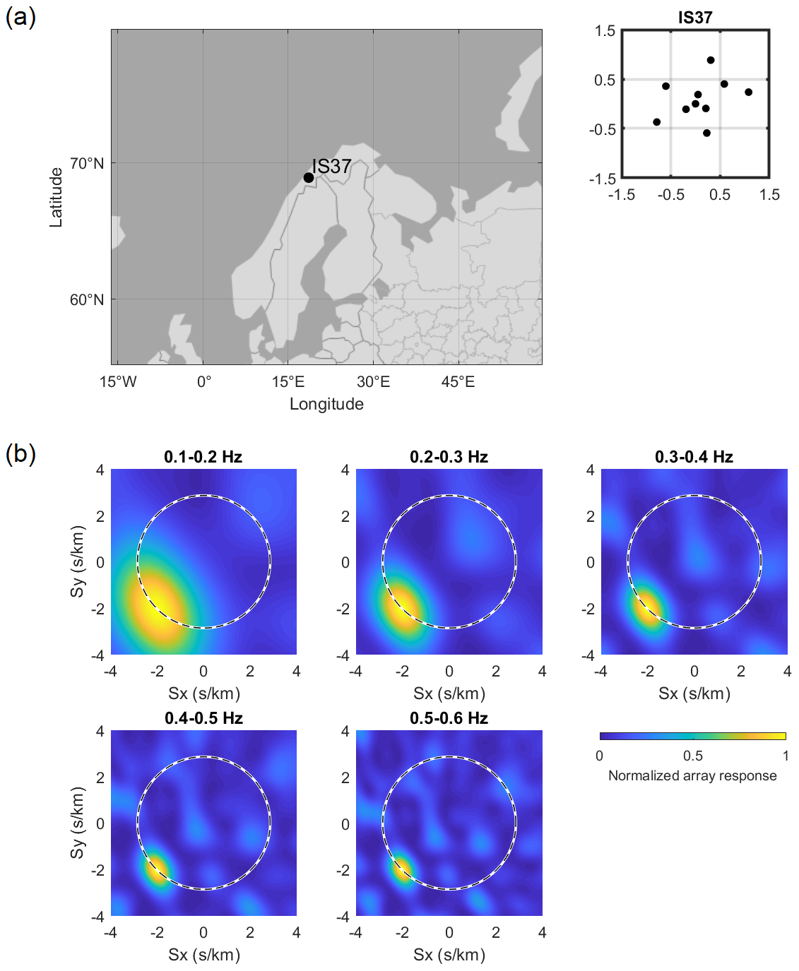
Figure 1(a) The IS37 infrasound array location and geometry. (b) Integrated steered array response for 0.1 Hz wide frequency bands, assuming a plane wave impinging at 225∘ back azimuth and 350 m s−1 apparent velocity (indicated with a dashed circle). Here Sx and Sy denote the horizontal components of the slowness vector.
2.1 Infrasound data set and signal processing
The infrasound array, denoted as IS37 or I37NO, is located in Bardufoss, Norway (69.07∘ N, 18.61∘ E), and is equipped with 10 MB3-type (MB2005 prior to 2016) microbarometers over an aperture of 2 km (Fig. 1a; Fyen et al., 2014). This station is part of the International Monitoring System (IMS) which verifies compliance with the Comprehensive Nuclear-Test-Ban Treaty (CTBT) (Dahlman et al., 2009; Marty, 2019). The station was certified by the CTBT Organization on 19 December 2013 and is operated by NORSAR, Kjeller, Norway (Schweitzer et al., 2021). Besides being included in the IMS, IS37 is also part of a regional network of European infrasound stations (Gibbons et al., 2007, 2015, 2019) that resolves significantly smaller events than the global IMS network (Le Pichon et al., 2008). In the framework of the regional network, data from IS37 have been used for multi-station studies characterizing European infrasound sources (e.g., Pilger et al., 2018).
The IS37 station routinely detects microbaroms within 0.1–0.6 Hz originating from the North Atlantic, the Barents Sea, and beyond. An analytical expression for a plane wavefront incident on the IS37 array was used to characterize the array's integrated, frequency-dependent response in 0.1 Hz wide frequency bands from 0.1 to 0.6 Hz. The wavefront was representative of a microbarom signal from the Atlantic Ocean, with a back azimuth of 225∘ and an apparent velocity of 350 m s−1, typical of the stratospheric regime (Garcés et al., 1998; Whitaker and Mutschlecner, 2008; Nippress et al., 2014; Lonzaga, 2015). The base resolution of the array was taken to be the 1σ beamwidth of the Gaussian fitted to the array response at a constant velocity of 350 m s−1 (dashed line in Fig. 1b) for each frequency band. The resulting resolution was found to be 35, 23, 16, 13, and 10∘ for 0.1–0.2, 0.2–0.3, 0.3–0.4, 0.4–0.5, and 0.5–0.6 Hz band, respectively. It should be noted that this estimate is based on the homogeneous medium plane wave time delays between the array elements only and does not take into account meteorological conditions at the station, noise, or other coherence loss mechanisms that may result in a wider beamwidth.
In array signal processing, the separation of coherent from incoherent parts of the recorded signal and the separation between different simultaneous arrivals are important concepts. When analyzing the wave field in terms of a given horizontal slowness vector (e.g., described in terms of apparent velocity and back azimuth), delay-and-sum beamforming (Ingate et al., 1985) is usually applied in combination with the underlying plane wave model assumption. This method applies time delays to the array sensor traces to focus on wavefronts arriving with a specific horizontal apparent velocity and a specific back azimuth direction, hence amplifying wave field components with the horizontal slowness of interest, while suppressing other components. However, the slowness vector models are not always accurate (Gibbons et al., 2020). In particular, the actual shape of the wavefront arriving at infrasound arrays may differ from a theoretical plane wave due to meteorological conditions and turbulence at the station, which make the underlying assumption of a locally homogeneous effective sound speed invalid. In this case, the beamforming is less efficient and the reduced array gain results in lower stack amplitude and signal distortion (Rost and Thomas, 2002).
To determine an unknown slowness vector component and to study the spatial structure of the wave field over time, one can use vespa (velocity spectral analysis) processing. This not only enhances the signal as the beamforming does but also allows one to determine either the direction or apparent velocity of the incoming signal. The vespa method estimates the power of the signal either for a fixed apparent velocity with varying back azimuth or for a fixed back azimuth with varying apparent velocity. The result of the vespa processing is usually presented as an image displaying the power of incoming signal as a function of time and back azimuth (or apparent velocity) called a vespagram. Although the vespa is widely applied in seismological array data studies (e.g., Davies et al., 1971; Kanasewich et al., 1973; Muirhead and Datt, 1976; McFadden et al., 1986), it has not previously been exploited in peer-reviewed microbarom infrasound studies.
The vespa-processing procedure described below is applied to each analyzed time window and frequency band as follows:
-
We extract, for each sensor n of an array, the signal trace xn(t) for the time window of interest. The analysis is done for a 1 h moving time window evaluated every 30 min. In general, the time series recorded at sensor n at the location rn can be written as follows:
where y(t) represents a plane wavefront, and shor is the horizontal component of the slowness vector
-
We remove the mean.
-
We apply a Butterworth bandpass filter to recordings. Calculations are performed for five equally spaced frequency bands that are within the microbarom frequency range (see Fig. 1b).
-
We compute beam traces or delay-and-sum traces of an array with N sensors as follows:
In this study, classical linear vespa processing (Davies et al., 1971) is applied, where the noise suppression is proportional to the square root of N (Rost and Thomas, 2002). A beam is generated at each 1∘ in back azimuth for the fixed apparent velocity of 350 m s−1. That allows us to estimate signals coming from all directions and from approximately the same height corresponding to stratospheric altitudes.
-
We calculate the mean squared pressure (power) of each beam to obtain an estimate of the incoming signal strength as a function of back azimuth and time.
Steps (1)–(5) are applied to all years of data analyzed. After the vespa processing, we apply a quality check based on the vespagram spectrum properties to exclude noisy data. At time windows when the vespa processing yields a directional spectrum with the power almost equal in all directions (the minimum exceeds 70 % of the maximum), data are ignored in our further analysis.
2.2 Microbarom source and propagation modeling
In this section, we summarize the approach applied to obtain the directional spectra of microbarom soundscapes as a function of time.
Ocean wave model. Hasselmann (1963) demonstrated that the nonlinear interactions between counter-propagating ocean waves can be presented as follows:
where H(f) is the interaction term spectrum known as the Hasselmann integral, E(fw,θ) is the power spectral density of the surface elevation, θ is the direction of the ocean wave propagation, fw is the wave frequency, and f is the acoustic frequency (). Ocean wave models estimate E(fw,θ) and its variations in space and time based on the surface wind fields. In this study, the WAVEWATCH III® (The WAVEWATCH III® Development Group, 2016) ocean wave model is considered (hereafter WWIII). The model grid resolution is 0.5∘ in latitude and longitude and 3 h in time. Among the WWIII output parameters is the p2l(fw) that represents the spectral density of the equivalent surface pressure that forces microbaroms as follows:
where ρ is the water density, and g is the gravity acceleration. Hence, the Hasselmann integral needed for further calculations can be obtained from the WWIII model using Eq. (4). Studies on microseisms (e.g., Hillers et al., 2012) have demonstrated the limitations of a model that does not account for coastal reflection. These limitations have been accordingly raised in the context of microbaroms (Landès et al., 2014). Therefore, in this study, the parametrization used to run the WWIII model accounts for fixed reflection coefficients of 10 % for the continents, 20 % for the islands, and 40 % for ice sheets (Ardhuin et al., 2011).
Microbarom source model. A microbarom source model is basically a model transforming an ocean wave model output into acoustic radiation spectrum in the atmosphere. Here, calculations are based on the model by De Carlo et al. (2020), taking into consideration both the finite ocean depth and the source radiation, depending on elevation and azimuth angles. This microbarom model allows the prediction of the location and intensity of the microbarom sources when applied to the Hasselmann integral. The output of this step is an acoustic spectrum for each cell of the wave model.
Microbarom propagation in the atmosphere. The next step is to account for the atmospheric influence on the microbarom propagation and ducting. For example, 3-D ray tracing or full-waveform approaches would provide an accurate simulation of the infrasound propagation; however, these methods involve a large computational burden (De Carlo et al., 2021). Instead, the semi-empirical attenuation law by Le Pichon et al. (2012) is used in the current study. The law is applied to the microbarom source spectra obtained in the previous step. This law accounts for the distance between the source and the station, as well as for the frequency, but assumes a horizontally homogeneous atmosphere. The atmospheric conditions at the station location are taken into account via Veff-ratio, which is the ratio of the effective sound speed in the propagation direction at 50 km altitude and the effective sound speed in the same direction on the ground. The atmospheric wind and temperature needed to determine the Veff-ratio are derived from the European Center for Medium-range Weather Forecasts (ECMWF) High-Resolution (HRES) forecast model (http://www.ecmwf.int, last access: 7 June 2021, Integrated Forecasting System – IFS; cycle 38r2). The atmospheric wind and temperature at the station location are extracted from a 0.5∘ × 0.5∘ model grid using bilinear interpolation. The temporal resolution of the ECMWF HRES forecast model is 6 h, and the assumption of the constant atmospheric wind and temperature over this time period is made to avoid a possible discrepancy caused by interpolation in time. The output of this step is an acoustic spectra attenuated to reflect what would be seen by the station.
Summation of sources. To obtain the directional spectrum at the station, all attenuated spectra from model cells within 1∘ azimuth band and less than 5000 km away from the station are summed. The distance limitation comes from the attenuation law definition. Although this attenuation law is widely used for propagation over very long distances (Smirnov et al., 2021; Pilger et al., 2019; Hupe et al., 2019; De Carlo et al., 2019), it was designed for distances up to 3000 km only. The choice of the maximum distance depends on the location of the station and the main sources, as well as on how realistic spectrum is needed for a specific task. Recently, De Carlo et al. (2021) provided a multi-station comparison between progressive multi-channel correlation (PMCC)-processed microbarom data and the microbarom model by De Carlo et al. (2020), which is also used in the current study. Results for 45 IMS stations in (De Carlo et al., 2021) demonstrate that integrating microbarom sources at distances up to 5000 km provides realistic spectra. Thus, all sources that are more than 5000 km away from the IS37 station are excluded from this study.
After applying these steps, and integrating over the frequency bands, we obtain an estimate of the microbarom power spectral density as a function of time and back azimuth, just as vespagrams. However, vespagrams cannot be directly compared to the modeled microbarom soundscapes since the latter do not take into account the frequency-dependent array resolution. Therefore, we smooth the modeled microbarom soundscapes by convolving with a Gaussian kernel at each time step, taking into account cyclical nature of back azimuth when smoothing near 360∘/0∘. Kernels are normalized to the unit area, and their standard deviations (width) decrease with frequency (see Sect. 2.1).
2.3 Similarity index
This section introduces an approach to benchmark the microbarom model against the infrasound data. Both data sets need to be of the same temporal resolution to assess a similarity at each time step. In the current study, in order to avoid interpolating the model output in time, the vespa processing output is sub-sampled to match the 3 h microbarom model grid. Hereinafter, all results are presented with a temporal resolution of 3 h.
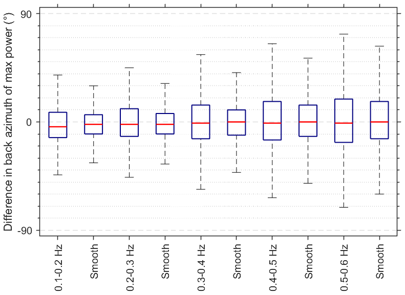
Figure 2Difference in the direction of the maximum power between (i) model and vespagram (indicated with a frequency band name on the x axis) and (ii) smoothed model and vespagram (denoted as “smooth” on the x axis) over 6 years of data. The red lines present the median, blue boxes indicate the 25 to 75 percentile range, and whiskers correspond to ± 3 standard deviations.
Figure 2 presents differences in the direction of the maximum power between the vespagram and either the model or the smoothed model. Both medians and uncertainty ranges are estimated based on the back azimuth difference at the maximum power only. Uncertainty values falling into the 25 to 75 percentile range are an objective assessment of the discrepancy between the model and vespagrams. These values originate from the wintertime when atmospheric conditions are favorable for the eastward ducting (Sect. 3.1). In summer, atmospheric conditions are not so stable (due to, e.g., increased cyclonic activity), and there are several factors that can cause model–vespagram discrepancies (Sect. 3.1) accompanied by an increase in the uncertainty range. Note that, after the smoothing (Sect. 2.2), there is a better agreement between the model and the vespagram, leading to a decrease in the median and the uncertainty ranges (Fig. 2).
A similarity index (SI), inspired by comparison approaches in image processing, is introduced as follows:
where MSE is the mean squared error (or difference) between the normalized smoothed model output, Pmodel(t,θ), and the normalized vespagram, Pvespa(t,θ), calculated at each time step, where θ is back azimuth, and t is time. This SI metric is, hence, insensitive to the total microbarom power but instead provides information on how accurate the model reproduces the directional pressure spectrum in the recorded data. A SI equal to one indicates a full match between model and infrasound vespagram in terms of the back azimuthal power distribution.
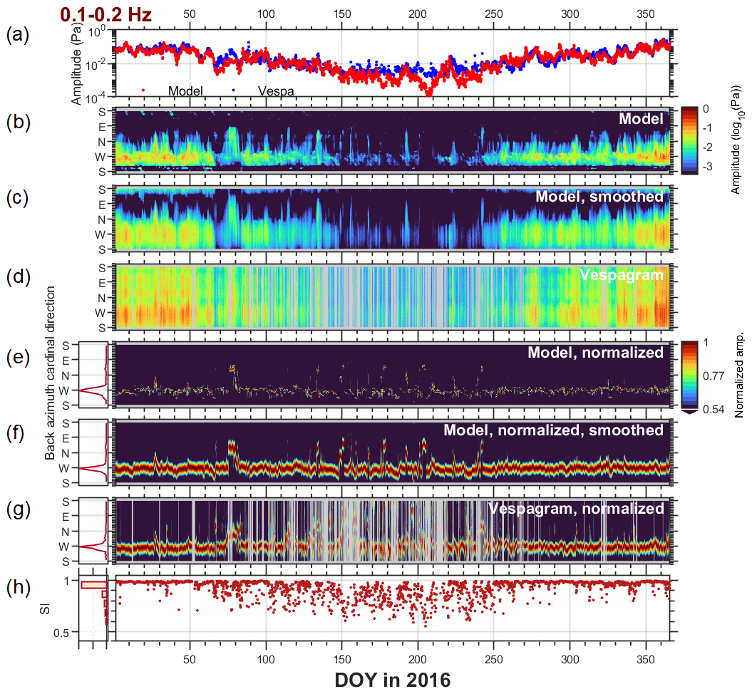
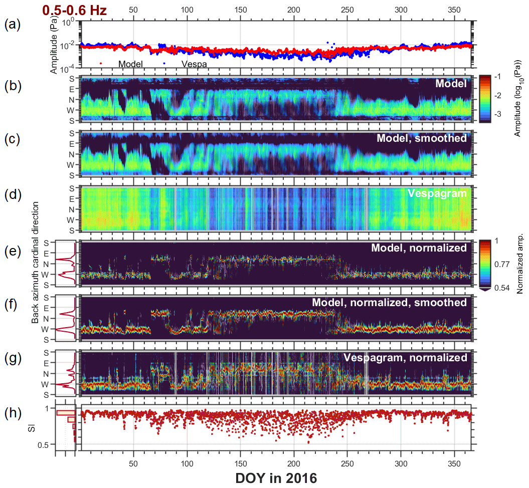
Figure 3Benchmarking microbarom model and infrasound vespagram for 0.1–0.2 Hz in 2016 for the IS37 station. (a) Amplitude of the dominant signal (blue – vespa processing; red – model). (b) The base 10 logarithm of the model amplitude. (c) The base 10 logarithm of the smoothed model amplitude (Sect. 2.2). (d) The base 10 logarithm of the infrasound vespagram amplitude (Sect. 2.1). The right-hand side panels in (e–g) are the same as panels (b–d) but after normalization by the maximum amplitude at each time step. The left-hand side panels in (e–g) show the normalized directional distribution of the dominant signal (10∘ bins). Panel (h) shows the similarity index between panels (f) and (g) (right) and the normalized distribution (left). Panels (b–d) have a common color bar, as do panels (e–g). Gray fields indicate periods where infrasound data are disregarded due to noise and an indistinct directional spectrum. Panels (b–g) are visualized using the Turbo color map (Mikhailov, 2019).
3.1 Comparison for full seasons
This section presents a multi-year model–vespagram comparison, focusing on microbarom characteristics over different seasons. We start with a detailed look at 2016 results, followed by an analysis of all 6 years.
Figures 3 and 4 present benchmarking microbarom model and vespa-processing images (vespagrams) for two frequency bands, namely 0.1–0.2 and 0.5–0.6 Hz, for 2016. These figures contain eight panels each, which are discussed in more detail below. Figures 3a and 4a show the maximum amplitude per time step over 1 year, i.e., the dominant signals in the azimuthal spectra. Enhanced ocean source activity during winter is accompanied by the eastward stratospheric wind favorable for ducting infrasound over long distances (Le Pichon et al., 2006). This results in a maximum of microbarom pressure amplitude both in model and vespagrams, regardless of the frequency band. The microbarom radiation model by De Carlo et al. (2020), combined with the semi-empirical wave attenuation law (Le Pichon et al., 2012), generally reproduces infrasound amplitudes accurately. An exception is between days 200 and 210 in 2016 (Fig. 3a), when the modeled amplitude is much lower than the amplitude obtained via the vespa processing. This discrepancy may indicate an overestimation of the attenuation caused by errors in the atmospheric model wind or due to the range-independent simplification.
Figures 3b–d and 4b–d display microbarom soundscapes as predicted by the model, smoothed model and vespa processed recordings, respectively. Here the soundscapes are plotted in terms of the base 10 logarithm of the amplitude, in order to allow the showing of the weaker summertime microbarom amplitudes in the same display as the stronger wintertime signals. Note that the vespagrams are noisier during summer (gray fields in Figs. 3g and 4g), especially for the 0.1–0.2 Hz band.
Due to the strong seasonal variability in the microbarom amplitude, it is difficult to compare the direction of winter to summer detections on an absolute amplitude scale. Thus, we normalize Figs. 3b–d and 4b–d by the maximum amplitude at each time step (see Figs. 3e–g and 4e–g; right) and estimate the directional distribution of the dominant signal in 10∘ bins (see Figs. 3e–g and 4e–g; left). For the frequency band of 0.1–0.2 Hz, the North Atlantic is the dominant source direction throughout the year (the main peak in Fig. 3e–g; left). However, the maximum power is sometimes also observed from northeasterly and southeasterly directions in summer. To generate infrasound at such low frequencies, the source needs to be of a substantial spatial extent, and therefore, there is a limited number of possible oceanic sources. After comparison with the model maps, we interpret these arrivals as microbaroms generated in the Pacific and Indian oceans, respectively. The stratospheric summertime westward wind could guide the infrasound waves towards the IS37 station. Unlike what is seen in the vespa-processed recordings, the model does not predict microbaroms originating from the Indian Ocean direction. A plausible reason for this is that the distance between the station and the Indian Ocean source region is ∼ 7000–8000 km, which is much greater than the maximum distance of 5000 km included in the modeling (see Sect. 2.2). Looking at higher frequencies, there is a pronounced change in the dominant direction of the source from the Atlantic in winter to the Barents Sea and the Greenland Sea in summer (peaks in Fig. 4e–g; left). This is associated with the change in wind direction in the stratosphere from eastward to westward. An analysis of a 6-year data set in terms of the dominant source direction indicates three prevailing microbarom source regions associated with the North Atlantic, the Greenland Sea, and the Barents Sea. These appear at the vespagram (model) back azimuths of 266 ± 14∘ (265 ± 16∘), 339 ± 14∘ (345 ± 8∘) and 26 ± 6∘ (34 ± 7∘).
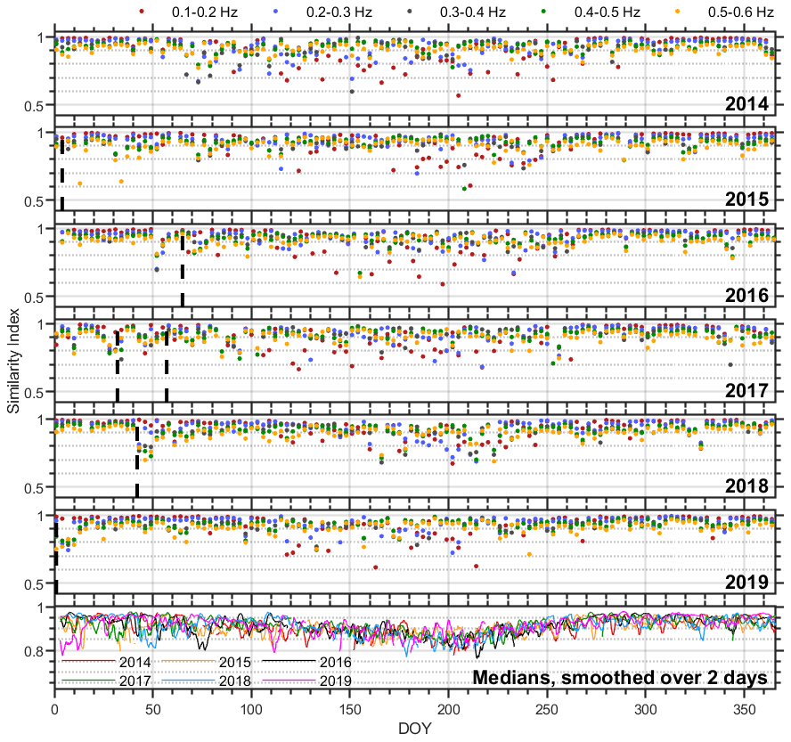
Figure 5Multi-year comparison between vespagrams and smoothed modeled microbarom soundscapes at the IS37 station. The similarity index is color-coded, depending on the frequency band, as follows: 0.1–0.2 Hz – red; 0.2–0.3 Hz – blue; 0.3–0.4 Hz – gray; 0.4–0.5 Hz – green; 0.5–0.6 Hz – orange. Data are presented as a discrete set with a time step of 3 d (day 1 – 00:00 UTC, day 4 – 00:00 UTC, etc.). Black dashed lines present SSW onsets. Medians over frequency bands in the last panel are color-coded, depending on the year, as follows: 2014 – red; 2015 – orange; 2016 – black; 2017 – green; 2018 – blue; 2019 – magenta.
Figures 3h and 4h present values of SI obtained over a year. In winter, SI for lower frequencies is stable and has values close to one, with exceptions corresponding to increased noise level in vespagrams or to sudden stratospheric warming (SSW) events that are discussed in Sect. 3.2. Relatively low SI for higher frequencies can be explained either by spurious apparent sources corresponding to array response function side lobes (Fig. 1b) or by the presence of local sources in the vespagram that are missed or not well reproduced in the model. In summer, SI values are quite variable and unstable but never fall below 0.5. Such behavior is typical regardless of the year or frequency band (see Fig. 5 for a multi-year comparison). One possible explanation is the changing weather conditions present at the station throughout the year. For example, Orsolini and Sorteberg (2009) have shown an enhancement in the number and intensity of summer cyclones in the Arctic and northern Eurasia. This would result in additional wind and rain noise in the infrasound recordings that would especially be enhanced at the lower frequencies. Another possible contribution would be the poor resolution of the array at low frequencies that can mix stratospheric signals with those from higher altitudes. These sometimes dominate at IS37 in summer (Näsholm et al., 2020) but are not included in the model. The relative stability of the model's results in Fig. 4e and f relative to the vespagram would indicate that there are additional sources of variability, either atmospheric, source region, or propagation path, that are not well characterized in the model.
As indicated by high SI values, especially in winter, the infrasound data processed in the framework of the vespa approach are in a good agreement with modeled microbarom soundscapes in both time (seasonal variations) and space (directional distribution). The similarity estimation proposed allows the detection of inconsistencies between the microbarom model and the vespa processing, which might be used for identifying biases in atmospheric models. This is especially promising for low frequencies where side lobes of the array response do not appreciably affect the analysis.
3.2 Examination of major sudden stratospheric warmings
Although this is not the main objective of the current study, in this section we examine the ability of the vespagrams to detect extreme atmospheric events, such as SSWs, and compare the model and the vespa processing for six selected events.
SSWs usually occur in wintertime and are, in general, associated with a sudden and short increase in stratospheric temperature and mesospheric cooling at high and middle latitudes (Shepherd et al., 2014; Butler et al., 2015; Limpasuvan et al., 2016; Zülicke et al., 2018). SSWs are often classified into minor and major warmings, depending on whether there was a weakening or reversal of the zonal wind (Butler et al., 2015). During the period of our consideration, three major and three minor SSWs occurred. Major SSWs took place with onsets on 5–6 March 2016 (Manney and Lawrence, 2016), 11 February 2018 (Rao et al., 2018; Lü et al., 2020), and 1 January 2019 (Rao et al., 2019, 2020), while the minor events occurred with onsets on 4 January 2015 (Manney et al., 2015; Mitnik et al., 2018) and 1 and 26 February 2017 (Eswaraiah et al., 2020). Note that there can be an error of up to several days in determining the SSW onset day, since there is no single way to define the onset, and different authors use different definitions. A prime example is the first SSW in 2017. According to the definition of the World Meteorological Organization, this event is classified as minor, but in a number of studies, it is referred to as major (Xiong et al., 2018; Conte et al., 2019). Vertical dashed lines in Figs. 5–6 correspond to the onset days listed above when SSW criteria were met.
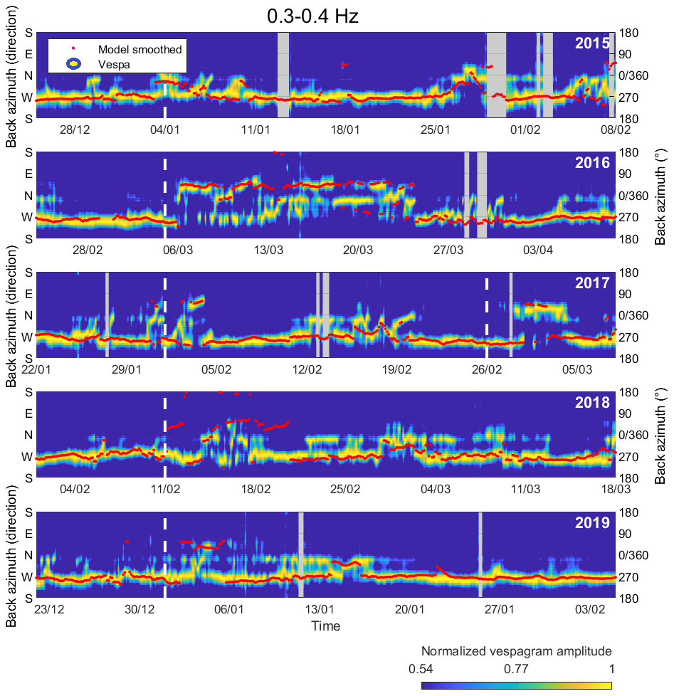
Figure 6Comparison between microbarom azimuthal distributions at IS37 (vespagrams) normalized per time step and the back azimuths of the dominant signals as predicted by the model (red dots). The results are shown around SSWs 2015–2019 for the 0.3–0.4 Hz band. White vertical dashed lines indicate onset days when SSWs (minor or major) criteria were met. Gray fields indicate periods where infrasound data are disregarded due to noise and an indistinct directional spectrum.
The infrasound signature reported by Donn and Rind (1971) and Evers and Siegmund (2009), which showed a significant change in direction of the infrasound arrival due to a change in favorable stratospheric waveguide, can be seen in Fig. 6 for all SSWs under consideration and in Figs. 3e–g and 4e–g for the 2016 SSW. The change in direction from the North Atlantic to the Barents Sea is clearly pronounced in both model and vespagrams around SSWs onset days. Figure 3f and g demonstrate that the signature appears late in the model data, and its duration is much shorter than in the vespagram, analogous to the study by Smets et al. (2016). For higher frequencies (Fig. 4f and g), the duration of a change from an eastward to a westward pattern is longer and continues until late March or early April, which corresponds to reanalysis data (Manney and Lawrence, 2016).
Another feature revealed is a significant decrease in similarity index between the model and vespagrams during SSWs (Fig. 5), which is characteristic for all events under consideration. The smallest discrepancies in the direction of the dominant wavefront between the model and infrasound data during SSWs reach about 5–7∘, but the largest reach as much as 90–100∘ (Fig. 6). This may be caused by the following factors. In most cases, the back azimuth change around SSWs onsets appears earlier in the vespagrams than in the model, with the difference of 3 to 24 h. Note that this also depends on the frequency band. Similar results were previously obtained by Smets and Evers (2014) and can be explained by the presence of an error in determining a SSW onset day from (re-)analysis data because of a scarcity of observations at stratospheric altitudes (Charlton-Perez et al., 2013) or by inadequate stratospheric analysis and forecast during SSWs, as addressed by Diamantakis (2014) and Smets et al. (2016). Sometimes the SSW signature does not appear in the vespagram while appearing in the model (see Fig. 6 around SSW 2018 onset day, for example). This can arise when employing a horizontally homogeneous atmosphere and overly constraining the model with the ECMWF wind and temperature at 50 km altitude. Such an approach does not allow a full, altitude-dependent description of infrasonic waves in the atmosphere and causes discrepancies between model and vespagrams. Considering long propagation path for microbaroms, net wind effect along the propagation path can be equal to zero in the vespagram, in contrast to the model, which estimates the probability of the signal arrival at the final point of the path. It has been demonstrated by Evers and Siegmund (2009) and Smets and Evers (2014) that the ECMWF wind direction does not always characterize the actual infrasound path, resulting in the abovementioned model–vespagram discrepancies.
Despite slight differences in the dominant direction of the wavefront arrival during SSW events, both model and vespagrams reproduce changes in the infrasound pattern correctly in time. Moreover, since vespagrams can detect changes in the stratospheric dynamics during extreme events, there is a potential for using it for near-real-time stratospheric diagnostics.
In this study, we compare observed and predicted microbaroms soundscapes using a vespagram-based approach. Analysis is performed based on the calculation of microbaroms power as a function of time and back azimuth at a constant apparent velocity of 350 m s−1. Note, however, that the vespagram family of time-dependent microbarom data visualizations can also be constructed using other array-processing techniques that estimate power as a function of the slowness of the wavefront, e.g., using robust estimators as explored by Bishop et al. (2020) or adaptive high-resolution approaches like Capon's method (Capon, 1969). An advantage of the vespagram approach is that microbarom radiation and propagation models can be benchmarked against recorded infrasound data for all directions simultaneously, as opposed to methods where only the back azimuth direction of maximum power is considered (e.g., Hupe et al., 2019; Smirnov et al., 2021). Since the vespa processing is computationally low cost and able to track variations in microbarom parameters over extended periods spanning 1 year or several years, it can be utilized for a near-real-time assessment of atmospheric model products and for developing infrasound-based stratospheric diagnostics. It can also be used when assessing changes in infrasound signatures over shorter time windows, e.g., during extreme atmospheric events.
Limitations in this study are predominantly related to microbarom propagation modeling. In addition to the scarcity of observations at the stratospheric altitudes (Charlton-Perez et al., 2013), which affect the accuracy of the directional distribution of predicted microbarom soundscapes, the horizontally homogeneous atmospheric approximation used in the study creates substantial limitations. In fact, the atmosphere is not homogeneous. It has horizontal and vertical inhomogeneities in the atmospheric wind and temperature fields caused, for example, by gravity waves, tides, and SSWs. These atmospheric disturbances significantly affect the long-distance infrasound propagation and, as a result, the directional spectra detected at the reception point. Moreover, the modeling would benefit from applying a full-waveform simulation code for the propagation of the radiated microbaroms to the station (e.g., Assink et al., 2014; Kim and Rodgers, 2017; Brissaud et al., 2017; Petersson and Sjögreen, 2018; Sabatini et al., 2019). This would provide a more refined modeling of the atmospheric ducting compared to the semi-empirical approach (Le Pichon et al., 2012) applied in the current study. An alternative, which is less computationally expensive, is (3-D) ray tracing, which can account for both range-dependent atmospheric models and cross-wind effects (e.g., Smets and Evers, 2014; Smets et al., 2016). However, the inherent high-frequency approximation of the ray theory can limit the modeling of diffraction and scattering effects (Chunchuzov et al., 2015) that can be important for the low-frequency microbaroms. Also note that more advanced simulations of infrasound propagation would require wind and temperature profiles with a high vertical resolution (or an appropriate stochastic parametrization) to account for the effect of small-scale atmospheric disturbances on microbarom scattering. Resolving small-scale structures in atmospheric models, reanalysis, and forecasting systems remains a topic of active research. Several research efforts were made to develop methods exploiting infrasound observations to improve the representation of wind and temperature in atmospheric model products (e.g., Chunchuzov et al., 2015; Assink et al., 2019; Amezcua et al., 2020; Vera Rodriguez et al., 2020).
A more elaborate microbarom propagation model could also allow for an estimate of the full microbarom wave field impinging an infrasound station and, hence, provide an estimate of its power within the full horizontal slowness space of plane wavefront directions (or a selected relevant region). In this way, we could benchmark modeled and recorded microbarom fields at an infrasound array for each sliding time window in the full horizontal slowness domain, without restricting the analysis to the region around a fixed apparent velocity as carried out in the current study. Notably, such “slowness plots” of modeled and recorded microbarom power are also (time-varying) images, which can be assessed and compared using the versatile ecosystem of image-processing and image comparison algorithms.
Future developments can include a compilation of long-term, time-dependent statistics of the similarities between model and infrasound recordings for multiple stations on global and regional scales. This would allow the definition of anomaly flag criteria, which would indicate unexpected inconsistencies between model and observations due to, for example, biases in atmospheric model products. Moreover, we suggest applying the approach presented here to global assessment and comparisons of ocean wave action model products, as well as to validate and further refine microbarom radiation estimation algorithms.
Figure A1 displays histograms of the apparent velocity detection statistics calculated using progressive multi-channel correlation (PMCC) processing (Cansi, 1995) for all frequency bands and years. These support the choice of 350 m s−1 as apparent velocity in the vespagram calculations for the analysis of microbaroms ducted through the stratosphere.
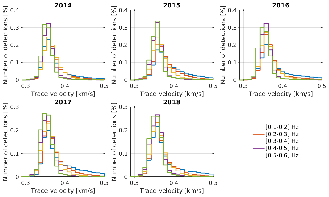
Figure A1Trace (apparent) velocity values as predicted by the PMCC for the IS37 infrasound station in 2014–2018. Frequency bands are color-coded as follows: blue – 0.1–0.2 Hz; orange – 0.2–0.3 Hz; yellow – 0.3–0.4 Hz; purple – 0.4–0.5 Hz; green – 0.5–0.6 Hz.
The IMS network's data can be accessed upon request through the virtual Data Exploitation Center (vDEC) via https://www.ctbto.org/specials/vdec (last access: 7 June 2021).
The high-resolution forecast model data, produced by the Integrated Forecast System of the ECMWF, can be accessed via https://www.ecmwf.int/en/forecasts/datasets (last access: 7 June 2021).
The modeled second-order equivalent surface pressure due to ocean wave interaction is available via ftp://ftp.ifremer.fr/ifremer/ww3/HINDCAST/SISMO/ (last access: 7 June 2021).
EV and SPN developed the vespagram calculation code, performed the infrasound data processing, and made the model and data analysis. MDC and ALP developed the microbarom model code and performed the simulations. EV prepared the paper, with contributions from all coauthors. PJE supervised the work and reviewed the results. SPN and ALP initiated the study.
The authors declare that they have no conflict of interest.
This study was facilitated by previous research performed within the framework of the ARISE and ARISE2 projects (Blanc et al., 2018, 2019), funded by the European Commission FP7 and Horizon 2020 programmes (grant nos. 284387 and 653980). The authors are thankful to Igor Chunchuzov and one anonymous reviewer, for valuable suggestions and constructive review of the paper. Ekaterina Vorobeva and Sven Peter Näsholm are also grateful to Yvan Joseph Orsolini, for the discussion and valuable comments.
This research has been supported by the Research Council of Norway (Norges Forskningsråd) programme (grant no. 274377) under the project of Middle Atmosphere Dynamics: Exploiting Infrasound Using a Multidisciplinary Approach at High Latitudes (MADEIRA).
This paper was edited by Gunter Stober and reviewed by Igor Chunchuzov and one anonymous referee.
Amezcua, J., Näsholm, S. P., Blixt, E. M., and Charlton-Perez, A. J.: Assimilation of atmospheric infrasound data to constrain tropospheric and stratospheric winds, Q. J. Roy. Meteor. Soc., 146, 2634–2653, https://doi.org/10.1002/qj.3809, 2020. a, b
Ardhuin, F., Stutzmann, E., Schimmel, M., and Mangeney, A.: Ocean wave sources of seismic noise, J. Geophys. Res.-Oceans, 116, C09004, https://doi.org/10.1029/2011JC006952, 2011. a
Assink, J., Smets, P., Marcillo, O., Weemstra, C., Lalande, J.-M., Waxler, R., and Evers, L.: Advances in infrasonic remote sensing methods, in: Infrasound Monitoring for Atmospheric Studies, edited by: Le Pichon, A., Blanc, E., and Hauchecorne, A., Springer, 605–632, 2019. a, b
Assink, J. D., Le Pichon, A., Blanc, E., Kallel, M., and Khemiri, L.: Evaluation of wind and temperature profiles from ECMWF analysis on two hemispheres using volcanic infrasound, J. Geophys. Res.-Atmos., 119, 8659–8683, 2014. a
Baird, H. F. and Banwell, C. J.: Recording of air-pressure oscillations associated with microseisms at Christchurch, NZJ Sci. Technol. Sect. B, 21, 314–329, 1940. a
Benioff, H. and Gutenberg, B.: Waves and currents recorded by electromagnetic barographs, B. Am. Meteorol. Soc., 20, 421–428, 1939. a, b
Bishop, J. W., Fee, D., and Szuberla, C. A. L.: Improved infrasound array processing with robust estimators, Geophys. J. Int., 221, 2058–2074, https://doi.org/10.1093/gji/ggaa110, 2020. a
Blanc, E., Ceranna, L., Hauchecorne, A., Charlton-Perez, A., Marchetti, E., Evers, L., Kvaerna, T., Lastovicka, J., Eliasson, L., Crosby, N., Blanc-Benon, P., Le Pichon, A., Brachet, N., Pilger, C., Keckhut, P., Assink, J., Smets, P. M., Lee, C., Kero, J., Sindelarova, T., Kämpfer, N., Rüfenacht, R., Farges, T., Millet, C., Näsholm, S. P., Gibbons, S., Espy, P., Hibbins, R., Heinrich, P., Ripepe, M., Khaykin, S., Mze, N., and Chum, J.: Toward an Improved Representation of Middle Atmospheric Dynamics Thanks to the ARISE Project, Surv. Geophys., 39, 171–225, https://doi.org/10.1007/s10712-017-9444-0, 2018. a, b
Blanc, E., Pol, K., Le Pichon, A., Hauchecorne, A., Keckhut, P., Baumgarten, G., Hildebrand, J., Höffner, J., Stober, G., Hibbins, R., Espy, P., Rapp, M., Kaifler, B., Ceranna, L., Hupe, P., Hagen, J., Rüfenacht, R., Kämpfer, N., and Smets, P.: Middle atmosphere variability and model uncertainties as investigated in the framework of the ARISE project, in: Infrasound Monitoring for Atmospheric Studies, edited by: Le Pichon, A., Blanc, E., and Hauchecorne, A., Springer, 845–887, 2019. a, b
Brekhovskikh, L.: Propagation of acoustic and infrared waves in natural waveguides over long distances, Sov. Phys. Uspekhi, 3, 159–166, https://doi.org/10.1070/pu1960v003n01abeh003263, 1960. a
Brekhovskikh, L. M., Goncharov, V. V., Kurtepov, V. M., and Naugolny, K. A.: Radiation of infrasound into atmosphere by surface-waves in ocean, Izv. An. SSSR Fiz. Atm+., 9, 899–907, 1973. a
Brissaud, Q., Martin, R., Garcia, R. F., and Komatitsch, D.: Hybrid Galerkin numerical modelling of elastodynamics and compressible Navier–Stokes couplings: applications to seismo-gravito acoustic waves, Geophys. J. Int., 210, 1047–1069, 2017. a
Büeler, D., Beerli, R., Wernli, H., and Grams, C. M.: Stratospheric influence on ECMWF sub-seasonal forecast skill for energy–industry-relevant surface weather in European countries, Q. J. Roy. Meteor. Soc., 146, 3675–3694, 2020. a
Butler, A. H., Seidel, D. J., Hardiman, S. C., Butchart, N., Birner, T., and Match, A.: Defining sudden stratospheric warmings, B. Am. Meteorol. Soc., 96, 1913–1928, 2015. a, b
Cansi, Y.: An automatic seismic event processing for detection and location: The PMCC method, Geophys. Res. Lett., 22, 1021–1024, 1995. a
Capon, J.: High-resolution frequency-wavenumber spectrum analysis, P. IEEE, 57, 1408–1418, 1969. a
Charlton-Perez, A. J., Baldwin, M. P., Birner, T., Black, R. X., Butler, A. H., Calvo, N., Davis, N. A., Gerber, E. P., Gillett, N., Hardiman, S., Kim, J., Krüger, K., Lee, Y.-Y., Manzini, E., McDaniel, B. A., Polvani, L., Reichler, T., Shaw, T. A., Sigmond, M., Son, S.-W., Toohey, M., Wilcox, L., Yoden, S., Christiansen, B., Lott, F., Shindell, D., Yukimoto, S., and Watanabe, S.: On the lack of stratospheric dynamical variability in low-top versions of the CMIP5 models, J. Geophys. Res.-Atmos., 118, 2494–2505, 2013. a, b
Chunchuzov, I., Kulichkov, S., Perepelkin, V., Popov, O., Firstov, P., Assink, J. D., and Marchetti, E.: Study of the wind velocity-layered structure in the stratosphere, mesosphere, and lower thermosphere by using infrasound probing of the atmosphere, J. Geophys. Res.-Atmos., 120, 8828–8840, 2015. a, b, c
Conte, J. F., Chau, J. L., and Peters, D. H. W.: Middle-and High-Latitude Mesosphere and Lower Thermosphere Mean Winds and Tides in Response to Strong Polar-Night Jet Oscillations, J. Geophys. Res.-Atmos., 124, 9262–9276, 2019. a
Dahlman, O., Mykkeltveit, S., and Haak, H.: Nuclear test ban: converting political visions to reality, Springer Science & Business Media, 2009. a
Davies, D., Kelly, E. J., and Filson, J. R.: Vespa process for analysis of seismic signals, Nature Physical Science, 232, 8–13, 1971. a, b, c
De Carlo, M., Le Pichon, A., Vergoz, J., Ardhuin, F., Näsholm, S. P., Ceranna, L., Hupe, P., and Pilger, C.: Characterizing ocean ambient noise in the North Atlantics and the Barents Sea regions, in: CTBTO Infrasound Technology Workshop (ITW), 2019. a, b
De Carlo, M., Ardhuin, F., and Le Pichon, A.: Atmospheric infrasound generation by ocean waves in finite depth: unified theory and application to radiation patterns, Geophys. J. Int., 221, 569–585, https://doi.org/10.1093/gji/ggaa015, 2020. a, b, c, d, e
De Carlo, M., Hupe, P., Le Pichon, A., Ceranna, L., and Ardhuin, F.: Global Microbarom Patterns: A First Confirmation of the Theory for Source and Propagation, Geophys. Res. Lett., 48, e2020GL090 163, https://doi.org/10.1029/2020GL090163, 2021. a, b, c, d
de Groot-Hedlin, C. D., Hedlin, M. A., and Drob, D. P.: Atmospheric variability and infrasound monitoring, in: Infrasound Monitoring for Atmospheric Studies, edited by: Le Pichon, A., Blanc, E., and Hauchecorne, A., Springer, 475–507, 2010. a
den Ouden, O. F. C., Assink, J. D., Smets, P. S. M., Shani-Kadmiel, S., Averbuch, G., and Evers, L. G.: CLEAN beamforming for the enhanced detection of multiple infrasonic sources, Geophys. J. Int., 221, 305–317, 2020. a
Dessauer, F., Graffunder, W., and Schaffhauser, J.: Über atmosphärische Pulsationen, Archiv für Meteorologie, Arch. Meteor. Geophy. B, 3, 453–463, 1951. a
Diamantakis, M.: Improving ECMWF forecasts of sudden stratospheric warmings, ECMWF Newsletter, 141, 30–36, 2014. a
Diamond, M.: Sound channels in the atmosphere, J. Geophys. Res., 68, 3459–3464, 1963. a
Domeisen, D. I. V., Butler, A. H., Charlton-Perez, A. J., Ayarzagüena, B., Baldwin, M. P., Dunn-Sigouin, E., Furtado, J. C., Garfinkel, C. I., Hitchcock, P., Karpechko, A. Y., Kim, H., Knight, J., Lang, A. L., Lim, E.-P., Marshall, A., Roff, G., Schwartz, C., Simpson, I. R., Son, S.-W., and Taguchi, M.: The Role of the Stratosphere in Subseasonal to Seasonal Prediction: 1. Predictability of the Stratosphere, J. Geophys. Res.-Atmos., 125, e2019JD030920, https://doi.org/10.1029/2019JD030920, 2020a. a
Domeisen, D. I. V., Butler, A. H., Charlton-Perez, A. J., Ayarzagüena, B., Baldwin, M. P., Dunn-Sigouin, E., Furtado, J. C., Garfinkel, C. I., Hitchcock, P., Karpechko, A. Y., Kim, H., Knight, J., Lang, A. L., Lim, E.-P., Marshall, A., Roff, G., Schwartz, C., Simpson, I. R., Son, S.-W., and Taguchi, M.: The Role of the Stratosphere in Subseasonal to Seasonal Prediction: 2. Predictability Arising From Stratosphere-Troposphere Coupling, J. Geophys. Res.-Atmos., 125, e2019JD030923, https://doi.org/10.1029/2019JD030923, 2020b. a
Donn, W. L. and Posmentier, E. S.: Infrasonic waves from the marine storm of April 7, 1966, J. Geophys. Res., 72, 2053–2061, 1967. a
Donn, W. L. and Rind, D.: Natural infrasound as an atmospheric probe, Geophys. J. Int., 26, 111–133, 1971. a
Dorrington, J., Finney, I., Palmer, T., and Weisheimer, A.: Beyond skill scores: exploring sub-seasonal forecast value through a case study of French month-ahead energy prediction, Q. J. Roy. Meteor. Soc., 146, 3623–3637, 2020. a
Eswaraiah, S., Kumar, K. N., Kim, Y. H., Chalapathi, G. V., Lee, W., Jiang, G., Yan, C., Yang, G., Ratnam, M. V., Prasanth, P. V., Rao, S. V. B., and Thyagarajan, K.: Low-latitude mesospheric signatures observed during the 2017 sudden stratospheric warming using the fuke meteor radar and ERA-5, J. Atmos. Sol.-Terr. Phy., 207, 105352, https://doi.org/10.1016/j.jastp.2020.105352, 2020. a
Evers, L. G. and Siegmund, P.: Infrasonic signature of the 2009 major sudden stratospheric warming, Geophys. Res. Lett., 36, L23808, https://doi.org/10.1029/2009GL041323, 2009. a, b
Fyen, J., Roth, M., and Larsen, P. W.: IS37 Infrasound Station in Bardufoss, Norway, NORSAR Scientific Report, 29–39, 2014. a, b
Garcés, M., Hansen, R. A., and Lindquist, K. G.: Traveltimes for infrasonic waves propagating in a stratified atmosphere, Geophys. J. Int., 135, 255–263, 1998. a
Garcés, M., Willis, M., Hetzer, C., Le Pichon, A., and Drob, D.: On using ocean swells for continuous infrasonic measurements of winds and temperature in the lower, middle, and upper atmosphere, Geophys. Res. Lett., 31, L19304, https://doi.org/10.1029/2004GL020696, 2004. a
Gibbons, S., Ringdal, F., and Kværna, T.: Joint seismic-infrasonic processing of recordings from a repeating source of atmospheric explosions, J. Acoust. Soc. Am., 122, EL158–EL164, 2007. a
Gibbons, S., Asming, V., Eliasson, L., Fedorov, A., Fyen, J., Kero, J., Kozlovskaya, E., Kværna, T., Liszka, L., Näsholm, S. P., Raita, T., Roth, M., Tiira, T., and Vinogradov, Y.: The European Arctic: A Laboratory for Seismoacoustic Studies, Seismol. Res. Lett., 86, 917–928, https://doi.org/10.1785/0220140230, 2015. a
Gibbons, S., Kværna, T., and Näsholm, S. P.: Characterization of the infrasonic wavefield from repeating seismo-acoustic events, in: Infrasound Monitoring for Atmospheric Studies, edited by: Le Pichon, A., Blanc, E., and Hauchecorne, A., Springer, 387–407, 2019. a
Gibbons, S. J., Kværna, T., Tiira, T., and Kozlovskaya, E.: A Benchmark Case Study for Seismic Event Relative Location, Geophys. J. Int., 223, 1313–1326, https://doi.org/10.1093/gji/ggaa362, 2020. a
Gutenberg, B. and Benioff, H.: Atmospheric-pressure waves near Pasadena, Eos T. Am. Geophys. Un., 22, 424–426, 1941. a
Hasselmann, K.: A statistical analysis of the generation of microseisms, Rev. Geophys., 1, 177–210, 1963. a
Hedlin, M., Walker, K., Drob, D., and de Groot-Hedlin, C.: Infrasound: Connecting the solid earth, oceans, and atmosphere, Annu. Rev. Earth Pl. Sc., 40, 327–354, 2012. a
Hibbins, R., Espy, P., and de Wit, R.: Gravity-Wave Detection in the Mesosphere Using Airglow Spectrometers and Meteor Radars, in: Infrasound Monitoring for Atmospheric Studies, edited by: Le Pichon, A., Blanc, E., and Hauchecorne, A., Springer, 649–668, 2019. a
Hillers, G., Graham, N., Campillo, M., Kedar, S., Landès, M., and Shapiro, N.: Global oceanic microseism sources as seen by seismic arrays and predicted by wave action models, Geochem. Geophy. Geosy., 13, Q01021, https://doi.org/10.1029/2011GC003875, 2012. a
Högbom, J. A.: Aperture synthesis with a non-regular distribution of interferometer baselines, Astron. Astrophys. Supp., 15, 417–426, 1974. a
Hupe, P., Ceranna, L., Pilger, C., De Carlo, M., Le Pichon, A., Kaifler, B., and Rapp, M.: Assessing middle atmosphere weather models using infrasound detections from microbaroms, Geophys. J. Int., 216, 1761–1767, 2019. a, b, c, d
Ingate, S. F., Husebye, E. S., and Christoffersson, A.: Regional arrays and optimum data processing schemes, B. Seismol. Soc. Am., 75, 1155–1177, 1985. a
Kanasewich, E. R., Hemmings, C. D., and Alpaslan, T.: Nth-root stack nonlinear multichannel filter, Geophysics, 38, 327–338, 1973. a
Kim, K. and Rodgers, A.: Influence of low-altitude meteorological conditions on local infrasound propagation investigated by 3-D full-waveform modeling, Geophys. J. Int., 210, 1252–1263, 2017. a
Landès, M., Le Pichon, A., Shapiro, N. M., Hillers, G., and Campillo, M.: Explaining global patterns of microbarom observations with wave action models, Geophys. J. Int., 199, 1328–1337, 2014. a
Le Pichon, A., Ceranna, L., Garcés, M., Drob, D., and Millet, C.: On using infrasound from interacting ocean swells for global continuous measurements of winds and temperature in the stratosphere, J. Geophys. Res.-Atmos., 111, D11106, https://doi.org/10.1029/2005JD006690, 2006. a
Le Pichon, A., Vergoz, J., Herry, P., and Ceranna, L.: Analyzing the detection capability of infrasound arrays in Central Europe, J. Geophys. Res.-Atmos., 113, D12115, https://doi.org//10.1029/2007JD009509, 2008. a
Le Pichon, A., Ceranna, L., and Vergoz, J.: Incorporating numerical modeling into estimates of the detection capability of the IMS infrasound network, J. Geophys. Res.-Atmos., 117, 1–12, https://doi.org/10.1029/2011JD016670, 2012. a, b, c, d
Le Pichon, A., Assink, J. D., Heinrich, P., Blanc, E., Charlton-Perez, A., Lee, C. F., Keckhut, P., Hauchecorne, A., Rüfenacht, R., Kämpfer, N., Drob, D. P., Smets, P. S. M., Evers, L. G., Ceranna, L., Pilger, C., Ross, O., and Claud, C.: Comparison of co-located independent ground-based middle atmospheric wind and temperature measurements with numerical weather prediction models, J. Geophys. Res.-Atmos., 120, 8318–8331, 2015. a
Le Pichon, A., Ceranna, L., Vergoz, J., and Tailpied, D.: Modeling the detection capability of the global IMS infrasound network, in: Infrasound Monitoring for Atmospheric Studies, edited by: Le Pichon, A., Blanc, E., and Hauchecorne, A., Springer, 593–604, 2019. a
Limpasuvan, V., Orsolini, Y. J., Chandran, A., Garcia, R. R., and Smith, A. K.: On the composite response of the MLT to major sudden stratospheric warming events with elevated stratopause, J. Geophys. Res.-Atmos., 121, 4518–4537, https://doi.org/10.1002/2015JD024401, 2016. a
Lonzaga, J. B.: A theoretical relation between the celerity and trace velocity of infrasonic phases, J. Acoust. Soc. Am., 138, EL242–EL247, 2015. a, b
Lü, Z., Li, F., Orsolini, Y. J., Gao, Y., and He, S.: Understanding of european cold extremes, sudden stratospheric warming, and siberian snow accumulation in the winter of 2017/18, J. Climate, 33, 527–545, 2020. a
Manney, G. L. and Lawrence, Z. D.: The major stratospheric final warming in 2016: dispersal of vortex air and termination of Arctic chemical ozone loss, Atmos. Chem. Phys., 16, 15371–15396, https://doi.org/10.5194/acp-16-15371-2016, 2016. a, b
Manney, G. L., Lawrence, Z. D., Santee, M. L., Read, W. G., Livesey, N. J., Lambert, A., Froidevaux, L., Pumphrey, H. C., and Schwartz, M. J.: A minor sudden stratospheric warming with a major impact: Transport and polar processing in the 2014/2015 Arctic winter, Geophys. Res. Lett., 42, 7808–7816, 2015. a
Marty, J.: The IMS infrasound network: current status and technological developments, in: Infrasound Monitoring for Atmospheric Studies, edited by: Le Pichon, A., Blanc, E., and Hauchecorne, A., Springer, 3–62, 2019. a
McFadden, P. L., Drummond, B. J., and Kravis, S.: The N th-root stack: Theory, applications, and examples, Geophysics, 51, 1879–1892, 1986. a
Mikhailov, A.: Turbo, An Improved Rainbow Colormap for Visualization, available at: https://ai.googleblog.com/2019/08/turbo-improved-rainbow-colormap-for.html (last access: 25 July 2020), 2019. a
Mitnik, L. M., Kuleshov, V. P., Pichugin, M. K., and Mitnik, M. L.: Sudden Stratospheric Warming in 2015–2016: Study with Satellite Passive Microwave Data and ERA5 Reanalysis, in: IGARSS 2018-2018 IEEE International Geoscience and Remote Sensing Symposium, 5556–5559, IEEE, 2018. a
Muirhead, K. J. and Datt, R.: The N-th root process applied to seismic array data, Geophys. J. Int., 47, 197–210, 1976. a
Näsholm, S. P., Vorobeva, E., Le Pichon, A., Orsolini, Y. J., Turquet, A. L., Hibbins, R. E., Espy, P. J., De Carlo, M., Assink, J. D., and Rodriguez, I. V.: Semidiurnal tidal signatures in microbarom infrasound array measurements, in: EGU General Assembly Conference Abstracts, Online, 4–8 May 2020, EGU2020-19035, https://doi.org/10.5194/egusphere-egu2020-19035, 2020. a
Nippress, A., Green, D. N., Marcillo, O. E., and Arrowsmith, S. J.: Generating regional infrasound celerity-range models using ground-truth information and the implications for event location, Geophys. J. Int., 197, 1154–1165, 2014. a
Orsolini, Y. J. and Sorteberg, A.: Projected changes in Eurasian and Arctic summer cyclones under global warming in the Bergen climate model, Atmospheric and Oceanic Science Letters, 2, 62–67, 2009. a
Petersson, N. A. and Sjögreen, B.: High order accurate finite difference modeling of seismo-acoustic wave propagation in a moving atmosphere and a heterogeneous earth model coupled across a realistic topography, J. Sci. Comput., 74, 290–323, 2018. a
Pilger, C., Ceranna, L., Ross, J. O., Vergoz, J., Le Pichon, A., Brachet, N., Blanc, E., Kero, J., Liszka, L., Gibbons, S., Kvaerna, T., Näsholm, S. P., Marchetti, E., Ripepe, M., Smets, P., Evers, L., Ghica, D., Ionescu, C., Sindelarova, T., Ben Horin, Y., and Mialle, P.: The European Infrasound Bulletin, Pure Appl. Geophys., 175, 3619–3638, 2018. a
Pilger, C., Gaebler, P., Ceranna, L., Le Pichon, A., Vergoz, J., Perttu, A., Tailpied, D., and Taisne, B.: Infrasound and seismoacoustic signatures of the 28 September 2018 Sulawesi super-shear earthquake, Nat. Hazards Earth Syst. Sci., 19, 2811–2825, https://doi.org/10.5194/nhess-19-2811-2019, 2019. a
Polavarapu, S., Shepherd, T. G., Rochon, Y., and Ren, S.: Some challenges of middle atmosphere data assimilation, Q. J. Roy. Meteor. Soc., 131, 3513–3527, 2005. a
Rao, J., Ren, R., Chen, H., Yu, Y., and Zhou, Y.: The stratospheric sudden warming event in February 2018 and its prediction by a climate system model, J. Geophys. Res.-Atmos., 123, 13–332, 2018. a
Rao, J., Garfinkel, C. I., Chen, H., and White, I. P.: The 2019 New Year stratospheric sudden warming and its real-time predictions in multiple S2S models, J. Geophys. Res.-Atmos., 124, 11155–11174, 2019. a
Rao, J., Garfinkel, C. I., and White, I. P.: Predicting the downward and surface influence of the February 2018 and January 2019 sudden stratospheric warming events in subseasonal to seasonal (S2S) models, J. Geophys. Res.-Atmos., 125, e2019JD031919, https://doi.org/10.1029/2019JD031919, 2020. a
Rienecker, M. M., Suarez, M. J., Gelaro, R., Todling, R., Bacmeister, J., Liu, E., Bosilovich, M. G., Schubert, S. D., Takacs, L., Kim, G.-K., Bloom, S., Chen, J., Collins, D., Conaty, A., da Silva, A., Gu, W., Joiner, J., Koster, R. D., Lucchesi, R., Molod, A., Owens, T., Pawson, S., Pegion, P., Redder, C. R., Reichle, R., Robertson, F. R., Ruddick, A. G., Sienkiewicz, M., and Woollen, J.: MERRA: NASA's modern-era retrospective analysis for research and applications, J. Climate, 24, 3624–3648, 2011. a
Rind, D., Donn, W. L., and Dede, E.: Upper air wind speeds calculated from observations of natural infrasound, J. Atmos. Sci., 30, 1726–1729, 1973. a
Rost, S. and Thomas, C.: Array seismology: Methods and applications, Rev. Geophys., 40, 2–1, 2002. a, b, c
Sabatini, R., Marsden, O., Bailly, C., and Gainville, O.: Three-dimensional direct numerical simulation of infrasound propagation in the Earth's atmosphere, J. Fluid Mech., 859, 754–789, 2019. a
Saxer, L.: Elektrische messung kleiner atmospharischer druckschwankungen, Helv. Phys. Acta, 18, 527–550, 1945. a
Saxer, L.: Über Entstehung und Ausbreitung quasiperiodischer Luftdruckschwankungen, Arch. Meteor. Geophy. B, 6, 451–463, 1954. a
Schweitzer, J., Fyen, J., Mykkeltveit, S., Gibbons, S. J., Pirli, M., Kühn, D., and Kværna, T.: Seismic arrays, in: New manual of seismological observatory practice 2 (NMSOP-2), Deutsches GeoForschungsZentrum GFZ, 1–80, 2012. a
Schweitzer, J., Köhler, A., and Christensen, J. M.: Development of the NORSAR Network over the Last 50 Yr, Seismol. Res. Lett., 92, 1501–1511, https://doi.org/10.1785/0220200375, 2021. a
Shepherd, M. G., Beagley, S. R., and Fomichev, V. I.: Stratospheric warming influence on the mesosphere/lower thermosphere as seen by the extended CMAM, Ann. Geophys., 32, 589–608, https://doi.org/10.5194/angeo-32-589-2014, 2014. a
Smets, P., Assink, J., and Evers, L.: The study of sudden stratospheric warmings using infrasound, in: Infrasound Monitoring for Atmospheric Studies, edited by: Le Pichon, A., Blanc, E., and Hauchecorne, A., Springer, 723–755, 2019. a
Smets, P. S. M. and Evers, L. G.: The life cycle of a sudden stratospheric warming from infrasonic ambient noise observations, J. Geophys. Res.-Atmos., 119, 12084–12099, https://doi.org/10.1002/2014JD021905, 2014. a, b, c, d
Smets, P. S. M., Assink, J. D., Le Pichon, A., and Evers, L. G.: ECMWF SSW forecast evaluation using infrasound, J. Geophys. Res.-Atmos., 121, 4637–4650, 2016. a, b, c
Smirnov, A., De Carlo, M., Le Pichon, A., Shapiro, N. M., and Kulichkov, S.: Characterizing the oceanic ambient noise as recorded by the dense seismo-acoustic Kazakh network, Solid Earth, 12, 503–520, https://doi.org/10.5194/se-12-503-2021, 2021. a, b, c
Smith, A. K.: Global dynamics of the MLT, Surv. Geophys., 33, 1177–1230, 2012. a
The WAVEWATCH III ® Development Group: User manual and system documentation of WAVEWATCH III ® version 5.16, Tech. Note 329, NOAA/NWS/NCEP/MMAB, 326 pp. + Appendices, 2016. a
Vera Rodriguez, I., Näsholm, S. P., and Le Pichon, A.: Atmospheric wind and temperature profiles inversion using infrasound: An ensemble model context, J. Acoust. Soc. Am., 148, 2923–2934, 2020. a
Waxler, R., Gilbert, K. E., Talmadge, C., and Hetzer, C.: The effects of the finite depth of the ocean on microbarom signals, in: 8th International Conference on Theoretical and Computational Acoustics (ICTCA), Crete, Greece, 2007. a
Whitaker, R. W. and Mutschlecner, J. P.: A comparison of infrasound signals refracted from stratospheric and thermospheric altitudes, J. Geophys. Res.-Atmos., 113, D08117, https://doi.org/10.1029/2007JD008852, 2008. a
Xiong, J., Wan, W., Ding, F., Liu, L., Hu, L., and Yan, C.: Two day wave traveling westward with wave number 1 during the sudden stratospheric warming in January 2017, J. Geophys. Res.-Space, 123, 3005–3013, 2018. a
Zülicke, C., Becker, E., Matthias, V., Peters, D. H. W., Schmidt, H., Liu, H.-L., de la Torre Ramos, L., and Mitchell, D. M.: Coupling of stratospheric warmings with mesospheric coolings in observations and simulations, J. Climate, 31, 1107–1133, 2018. a