the Creative Commons Attribution 4.0 License.
the Creative Commons Attribution 4.0 License.
 | 12 May 2021
Planetary radar science case for EISCAT 3D
Torbjørn Tveito
Juha Vierinen
Björn Gustavsson
Viswanathan Lakshmi Narayanan
Ground-based inverse synthetic aperture radar is a tool that can provide insights into the early history and formative processes of planetary bodies in the inner solar system. This information is gathered by measuring the scattering matrix of the target body, providing composite information about the physical structure and chemical makeup of its surface and subsurface down to the penetration depth of the radio wave. This work describes the technical capabilities of the upcoming 233 MHz European Incoherent Scatter Scientific Association (EISCAT) 3D radar facility for measuring planetary surfaces. Estimates of the achievable signal-to-noise ratios for terrestrial target bodies are provided. While Venus and Mars can possibly be detected, only the Moon is found to have sufficient signal-to-noise ratio to allow high-resolution mapping to be performed. The performance of the EISCAT 3D antenna layout is evaluated for interferometric range–Doppler disambiguation, and it is found to be well suited for this task, providing up to 20 dB of separation between Doppler northern and southern hemispheres in our case study. The low frequency used by EISCAT 3D is more affected by the ionosphere than higher-frequency radars. The magnitude of the Doppler broadening due to ionospheric propagation effects associated with traveling ionospheric disturbances has been estimated. The effect is found to be significant but not severe enough to prevent high-resolution imaging. A survey of lunar observing opportunities between 2022 and 2040 is evaluated by investigating the path of the sub-radar point when the Moon is above the local radar horizon. During this time, a good variety of look directions and Doppler equator directions are found, with observations opportunities available for approximately 10 d every lunar month. EISCAT 3D will be able to provide new, high-quality polarimetric scattering maps of the nearside of the Moon with the previously unused wavelength of 1.3 m, which provides a good compromise between radio wave penetration depth and Doppler resolution.
- Article
(2353 KB) - Full-text XML
- Companion paper
- BibTeX
- EndNote


Ground-based radio remote sensing of planetary surfaces is a remote sensing technique wherein a planetary target is illuminated by a radar transmitter on the surface of Earth. This is a tool that can provide insights into the formative processes of the surfaces of the inner planets and the conditions in the early history of the solar system (Ostro, 1993; Campbell, 2016). Radar mapping of planetary surfaces provides information about the properties of the upper layers of the planet's surface and can also provide accurate information about an object's rotation (Campbell et al., 2019). Actively transmitting the radio wave allows researchers to control the frequency, amplitude, and polarization of the illuminating beam. This means that we can extract information about the surface from the ways in which it affects these parameters. Remote sensing techniques are often an inexpensive, less-resource-intensive alternative to in situ measurements for obtaining information about large swathes of planetary surfaces.
It is impossible to summarize all of the scientific highlights of previous planetary radar research here. However, we have tried to list topics that may be interesting to study using European Incoherent Scatter Scientific Association (EISCAT) 3D. Previous lunar radio remote sensing studies have been used to determine the average roughness of the lunar surface on several length scales and to investigate the geology of the upper crust of the lunar nearside (Evans and Hagfors, 1968). Radar studies of planetary targets in the solar system have been used to look for water ice in permanently shadowed craters (Campbell, 2016). These craters tend to be near the poles, where the crater rims shields the interior from sunlight. Spudis et al. (2013), using the mini-RF (radio frequency) instrument on board the Lunar Reconnaissance Orbiter, found evidence of such water deposits near the lunar poles. Radar-bright features consistent with water ice have been found on Mercury's permanently shadowed polar craters (Harmon et al., 2011) using only the Arecibo radar. Radar studies have also been used to map the surface of Venus through its visually opaque clouds and determine its retrograde rotation (Goldstein and Carpenter, 1963). These maps revealed a surface dominated by volcanism, with a large number of shield volcanoes and relatively few craters. This suggested that the planet was geologically active relatively recently, and may still be (Phillips et al., 1992). A continuing radar campaign aimed at looking for changes in the Venusian landscape could give information regarding the temporal and spatial scale of geologic activity (Shalygin et al., 2012).
The use of many different wavelengths for investigating planetary surfaces is important in order to build a more complete understanding of the properties of the target body (Thompson, 1979). This is because the radio wave is modified by spatial variations in the dielectric constant of the medium it interacts with. These variations can be caused by both structural and compositional variations in the medium. Specular scattering is dominated by smooth surfaces normally oriented to the radar line of sight. Structural variations of the order of 10 % to 100 % of the wavelength contribute the majority of the depolarized component of the reflected signal. Simultaneously, the wave will attenuate when it penetrates the target body. The penetration depth is the point at which the power of the wave is reduced to e−1 and is roughly proportional to the wavelength used to investigate (Campbell, 2002). These two effects, in tandem, mean that different wavelengths provide different, complementary slices of information. Another parameter that is affected by the frequency of the illuminating wave is the Doppler resolution achievable. Longer wavelengths are not able to obtain as fine a resolution as shorter wavelengths if observation times are the same.
There are several different types of ground-based radar remote sensing experiments of planetary targets. Range–Doppler mapping of radio albedo can provide information about the structural and dielectric properties of the surface of the body being observed. If polarimetric information is available, the near subsurface can be partially separated from the surface echo, providing more information about the subsurface structure and chemical composition. If several receivers are available, topographical mapping is possible by using the phase difference between the received signals to calculate differences in optical path length (Margot et al., 2000). This type of interferometric calculation can also be used to resolve ambiguities in range–Doppler mapping caused by target geometries (Rogers and Ingalls, 1969). Radar measurements can also be used to ascertain the distance to an object, and its relative velocity. Repeated measurements can then help constrain the orbital characteristics of near-Earth objects (NEOs), identifying potentially hazardous space objects (Giorgini et al., 2008). Radar observations of asteroids can also aid in determining their spin state through investigating Doppler spectra or radar speckle patterns (Busch et al., 2010). A detailed analysis of the capabilities of EISCAT 3D in relation to observation of NEOs has been done in a companion paper by Kastinen et al. (2020).
Previous long-wavelength, ground-based inverse synthetic aperture radar maps of the lunar surface include a map of backscatter at 40 MHz (7.5 m) by Thompson (1978). This observation provided the first high-resolution map of the lunar nearside for long-wavelength radar and a measurement of the average scattering properties of the lunar regolith at long wavelengths. A recent study by Vierinen et al. (2017b) provided a view of the lunar nearside at 6 m, where both the specular and orthogonal-to-specular polarizations were recorded. This gives a view of the properties of both the surface and subsurface. The long-wavelength studies have identified two regions, namely (1) the Schiller–Zucchius basin and (2) the highlands around Montes Jura, which have anomalously low depolarized radar returns (Thompson et al., 2006; Vierinen et al., 2017b). The use of 230 MHz radar maps would be of interest in order to constrain the physical mechanism that causes this reduced return.
In this paper, we discuss the upcoming EISCAT 3D radar facility and its capabilities in the context of planetary radar studies. In Sect. 2, we describe the performance parameters of the radar. Section 3 investigates the detectability of Mars, Venus, and Mercury, as well as the Moon. In Sect. 4, we discuss an interferometric technique for disambiguating Doppler north and south from one another and estimate the achievable contrast obtainable using the EISCAT 3D interferometer. In Sect. 5, we investigate how severely ionospheric radio propagation will degrade the Doppler resolution radar maps. This is done using a first-order model for traveling ionospheric disturbances. Section 6 outlines Lunar observing opportunities between 2022 and 2040 using EISCAT 3D.
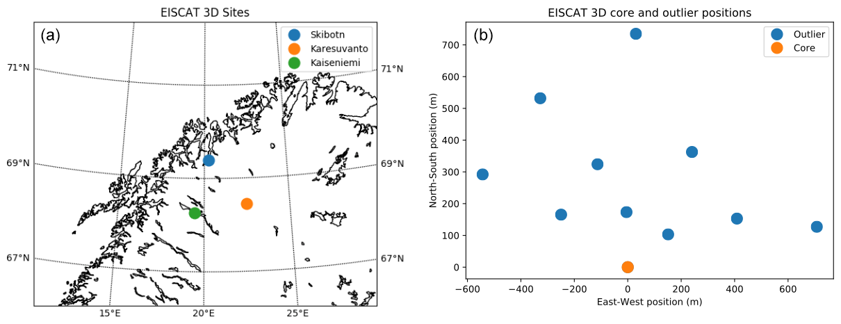
Figure 1(a) Locations of the three receiver sites of EISCAT 3D. The Skibotn site has both transmitting and receiving capabilities, while the Kaiseniemi and Karesuvanto are only able to receive. (b) Planned distribution of antenna modules at the Skibotn site. Note that only the Skibotn site is planned to have outlier antenna modules intended for interferometric purposes.
EISCAT 3D is a new, multi-static, high power, large aperture-phased array radar scheduled for first-light experiments in 2022. The facility is currently being built in northern Fennoscandia, with the transmitter located in Skibotn, Norway, as can be seen in Fig. 1. The primary science case for this new facility is ionospheric and upper atmospheric physics (McCrea et al., 2015). However, this radar will also potentially be very useful for planetary radar studies.
The radar facility will be able to transmit and receive signals at elevations down to 30∘ above the horizon. This will allow both a view of the ecliptic plane and lunar observations of several hours. The facility will operate with a 233 MHz center frequency, a 5 MHz transmit bandwidth, a 30 MHz receive bandwidth (Vierinen et al., 2017a), a system noise temperature of 150 K, a peak transmit power of 5 MW, and a maximum duty cycle of 25 % (Kero et al., 2019). The main antenna arrays have a maximal diameter of 75 m and a maximal gain, G0, of 43 dB towards zenith. The decline in gain as a function of angle of incidence can be approximated as the reduction in projected area, G=G0cos θ. The radar allows independent transmission and reception on two orthogonal linear polarizations. As a consequence of this, any polarization state vector can be synthesized. The wavelength has not, to our knowledge, been used previously for lunar studies. This means that the radar will be able to sample a new scale size in lunar surface roughness and subsurface structure.
Another benefit of the EISCAT 3D facility is the availability of numerous interferometric baselines, with distances over 100 km being possible (see Fig. 1 for the planned configuration of antenna placement). The Skibotn antenna location will have 10 outlier antenna modules, each with a maximal diameter of approximately 7.9 m, consisting of 91 dipole antenna elements. While these additional antenna modules do not provide as high a signal-to-noise ratio, they can be useful in providing a large number of interferometric baselines. In total, when using all three receiving sites and the Skibotn outlier antennae, one can create 78 unique antenna pairs.
The relatively low elevation angle of the lunar face presents three challenges for radar imaging. (1) The antenna gain pattern will be elongated in the elevation direction. This will cause a loss of signal strength. (2) The elevation pointing direction will also cause a polarization-dependent phase and an amplitude response for the antenna. This will require careful calibration. (3) The point spread function of the interferometer will also be affected.
Of these effects, the polarization-dependent antenna response is probably most important. This will most likely require the community to develop an azimuth and elevation-dependent polarization response model for the EISCAT 3D antenna.
In this section, we evaluate the signal-to-noise ratios (SNRs) of planetary bodies when observed by EISCAT 3D. The SNR ρ is found as follows:
The first term is a constant, the second term describes the specifics of the radar system, the third term is target-specific factors, and the last term is the square root of the observation time. The expression for the SNR for a planetary target is given by Ostro (1993). These expressions are also derived and discussed in a companion paper by Kastinen et al. (2020), in the context of detectability of NEOs using the EISCAT 3D facility.
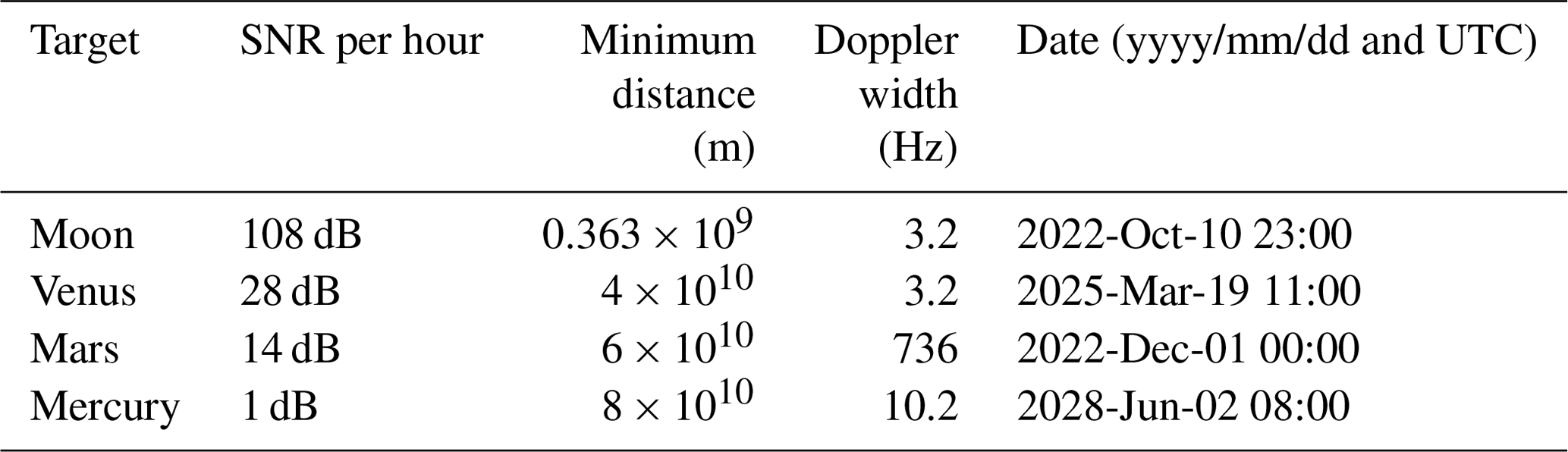
Table 1 lists the highest SNR observing opportunities for the three other terrestrial planets and the Moon during the period 2022–2032. The table lists the date of observation, SNR, estimated Doppler width, and range to the center of the target body. We used the NASA HORIZONS ephemeris (Giorgini et al., 2001) to find the elevation angle for each planetary body once per hour over the time period, and we evaluated the closest pass for each body that was above the 30∘ cut-off elevation. We then calculated the SNR using the expression found in Ostro (1993) and Kastinen et al. (2020), with a 25 % duty cycle, and assuming a 0.1 radar albedo. While it is customary to report SNR obtained during the time it takes for the radar signal to make a round-trip to the target and back, we used SNR per hour, as the 25 % duty cycle allows for interleaved transmit and receive.
It is obvious from Table 1 that only the Moon is a viable radar target. The other terrestrial planets are simply too faint for scientific mapping purposes. While Venus and Mars may be detectable, they cannot be used to produce a range–Doppler radar image with a sufficient number of pixels.
Target selection is limited by the achievable SNR. Due to the R−4 dependence of the returned signal, distant objects quickly become lost in noise. In order to compensate for the low signal of distant objects, one can increase the effective collecting area of the radar receiver. It would, therefore, be possible that future expansions of the EISCAT 3D facility allows the study of more distant objects. In order to make a meaningful difference, the product of transmit power, gain, and receiver aperture would need to be increased by several orders of magnitude. Such an expansion may prove to be challenging in practice.
Table 1Achievable SNR for hour-long observations of the terrestrial planets and the Moon. The date at which the target has the best SNR is shown (in yyyy/mm/dd and universal coordinated time – UTC), along with the Doppler width and approximate distance during the observation period.
The small solar elongation angle to Mercury and Venus will probably increase the receiver noise significantly, as the Sun will often be relatively close to the radar antenna beam axis. Therefore, the SNR for Mercury and Venus are probably overestimated.
While the SNR calculations indicate that it may be possible to detect Venus, Mars, and Mercury with the E3D, they are not mappable radar targets. Assuming Venus has an SNR of 28 dB, this will only produce a radar map with approximately 8×8 pixels with an SNR of 10 dB per pixel. While it is possible to increase the SNR through increasing total integration time, this increase is approximately linear. The total amount of time required to obtain useful resolutions is so high as to not be worth attempting.
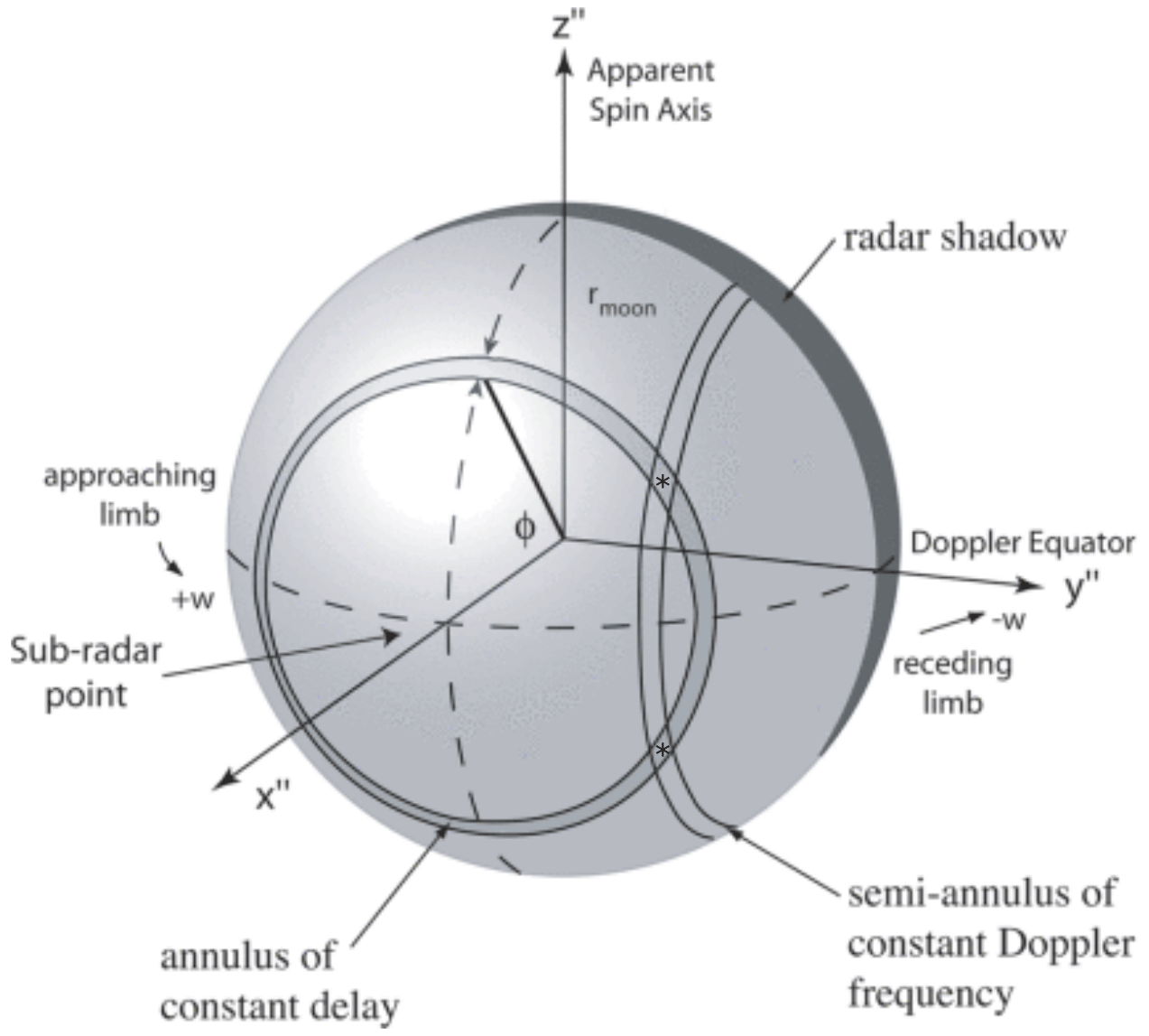
Figure 2In this figure, the geometry of range–Doppler mapping is shown. Each range pixel takes the form of a ring on the surface of the Moon, centered on the sub-radar point. Each frequency bin takes the form of a ring, centered on the equator, 90∘ east and west of the sub-radar point. Marked with a star are two regions that will have the same range and Doppler dimensions and are symmetrical to the Doppler equator. These regions are indistinguishable with only range and Doppler information, and every point on the apparent northern hemisphere will have a point on the southern hemisphere with identical range and Doppler coordinates. Figure adapted from Campbell et al. (2007).
The range–Doppler ambiguity can be seen in Fig. 2. Every point on the northern (positive z′′ direction) hemisphere is identifiable by one ring of constant range and one ring of constant Doppler shift. These rings also intersect on the southern hemisphere, assuming that the target is spherical. This means that any range–Doppler coordinate pair points to two physical locations, namely one north of the apparent Doppler equator and one to the south. Untreated range–Doppler maps therefore appear to fold along the equator, adding together the regions on both hemispheres that have the same range and Doppler values. This folding makes it challenging to extract useful information from the maps.
The range–Doppler north–south ambiguity can be removed by an interferometric technique described by Rogers and Ingalls (1969). This method relies on using the phase difference between two receiving antennae to discriminate between echoes from the ambiguous points. While Rogers and Ingalls originally used only one interferometric antenna pair, the method can be expanded to an arbitrary number of unique pairs. The addition of more antennae with different interferometric baselines makes the inverse problem of separating Doppler north from Doppler south more overdetermined. Discussing the interferometry in detail is out of the scope of this paper. We refer you to a companion paper by Stamm et al. (2020) for a discussion on the interferometric imaging capabilities of EISCAT 3D. Disambiguation by selectively illuminating only one hemisphere at a time is not viable due to the beamwidth being significantly larger than the angular extent of the Moon.
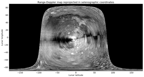
Figure 3Due to uncertainties in the disambiguation calculation, a band surrounding the Doppler equator is poorly resolved. Note that the map is reprojected from range and Doppler coordinates to selenographic coordinates. Near the Doppler equator, features become lost in noise due to the noise-enhancing effects of poor disambiguation. This figure is produced from the same data as Vierinen et al. (2017b).
When using a two-antenna interferometer to disambiguate the Doppler north and south, there is a region near the Doppler equator where the angular separation between the Doppler north and south region is very small. As the phase difference approaches zero near the Doppler equator, there will be a region surrounding it where the north–south ambiguity is unresolvable. The width of this gap to the first order is inversely proportional to the separation of the antennas. An example of such a band is shown in Fig. 3. This map is made by Vierinen et al. (2017b) using data gathered by the Jicamarca radar facility, using a single interferometric antenna pair.
Due to the increased number of elements in the EISCAT 3D interferometer, and the availability of extremely long baselines, this ambiguous band will be significantly smaller. In combination with the regular and frequent observation opportunities, this means that EISCAT 3D could map the reflectivity of the low-latitude, low-longitude region of the lunar nearside.
The data for the 2017 study by Vierinen et al. was collected with the Jicamarca radio observatory using the northernmost and southernmost modules, giving a baseline of 424 m. There are 64 modules, with side lengths of approximately 40 m each. With a 6 m wavelength, this gives an approximate gain of 27.5 dB at normal incidence. The EISCAT 3D outlier antennae are hexagonal with a maximal diameter of approximately 7.9 m with a wavelength of 1.3 m. We will assume that this also gives a gain of 27.5 dB at normal incidence. Due to the improved steering of the EISCAT facility over Jicamarca, targets are viewable at 30∘ elevation from the horizon. This reduces the effective collecting area of the antenna but also increases the possible observation time.
Interhemispheric cross talk is the power from one hemisphere that is incorrectly measured as coming from the other hemisphere. In order to estimate this for EISCAT 3D, we will be using the set of equations provided by Vierinen et al. (2017b) in Appendix 1. We will assume that the power only originates from one hemisphere, such that pn=0 and ps=1, meaning that all of the power measured is originating from the southern hemisphere. The estimate of interhemispheric cross talk then becomes the following:
where σn is the a posteriori standard deviation of the measured power from the northern hemisphere and μ is our estimate of interhemispheric cross talk. A higher value for μ would mean that a larger amount of the power estimated to be originating from the northern hemisphere is actually from the southern hemisphere.
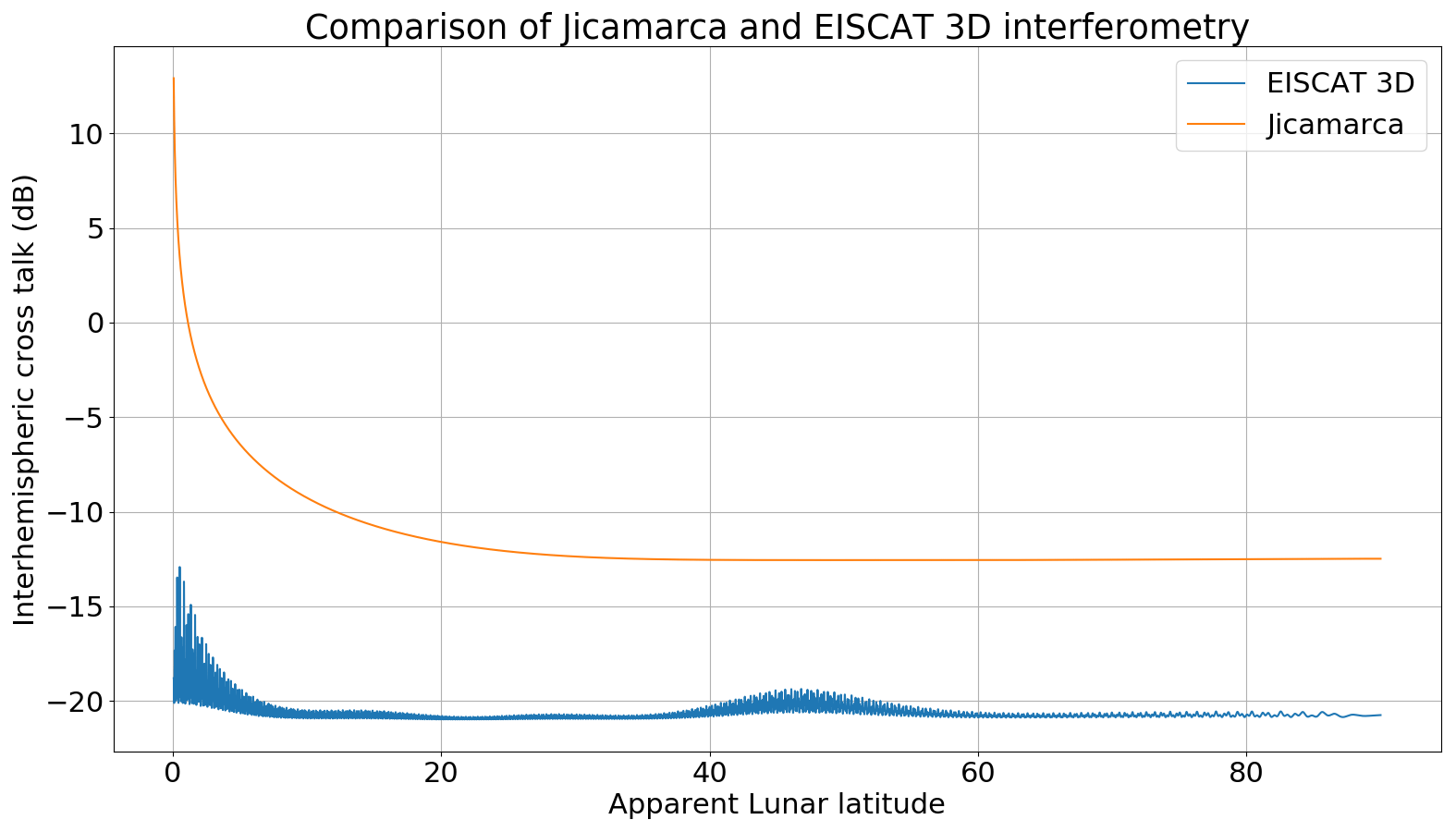
Figure 4A comparison of interhemispheric cross talk (Eq. 2) between the configuration used by Vierinen et al. (2017b), using the Jicamarca radio observatory, and the EISCAT 3D facility and every unique interferometric baseline larger than 50 m. The apparent lunar latitude is terminated at approximately 0.05∘. Note that the estimate for EISCAT 3D is lower, at all points, than what is estimated for Jicamarca, which suggests that even regions close to the Doppler equator should be possible to disambiguate with the interferometric capabilities of EISCAT 3D.
The reduction in gain at 30∘ elevation is proportional to the reduction in projected area, leaving the total gain at approximately 24 dB, which should be more than sufficient for lunar observations. As the outlier antennae have sufficient gain to act as interferometers, there are a total of 78 possible unique baselines. For our lunar calculations, we have assumed that the Doppler axis is aligned with Earth's and excluded any baseline less than 50 m in the north–south direction to shorten calculation time.
In Fig. 4, we have evaluated the interferometric performance for EISCAT 3D and Jicamarca as a function of lunar latitude. The interferometric performance is measured with interhemispheric cross talk, μ, which is given in Eq. (2). From the figure, we can see that the EISCAT 3D achieves an interhemispheric cross talk of approximately −20 dB. As a point of comparison, the Jicamarca Radio Observatory only attains −12 dB. This means that it is comparatively easier to distinguish between points on the northern and southern hemispheres. This is due to the significantly larger number of interferometer baselines available with EISCAT 3D, making the linear regression problem of separating the Doppler north and south a highly overdetermined problem. In the calculation of interhemispheric cross talk, we have assumed that both EISCAT 3D and Jicamarca make 81 independent power measurements, as was done in the previous Jicamarca study (Vierinen et al., 2017b).
Therefore, as a consequence of the diversity of interferometer baselines, the ambiguous band will be significantly thinner with the EISCAT 3D radar than with the previous Jicamarca observation, allowing us to see regions quite near to the apparent equator. If observations are conducted some time apart, it is possible to sample the lunar surface with different sub-radar points and apparent equators. If the apparent lunar rotation is in a different direction in two different maps, the unresolved band about the Doppler equator will fall in different regions of the Moon. The same is also true for maps with different sub-radar points. This means that if one is attempting to create a map with total coverage of the lunar nearside, a thin unresolved region means that fewer unique looks are required.
The relatively long wavelength used by EISCAT 3D also provides a challenge in that it is affected by more than shorter wavelengths in the Earth's ionosphere. Spatial variations in the plasma density cause spatial variations in the refractive index. The refractive index is found from the Appleton–Hartree equation which, for an unmagnetized, collisionless plasma can be simplified to the following:
where n is the refractive index, fp is the plasma frequency, and f is the frequency of the electromagnetic wave. In our case, the radar frequency is 233 MHz, and typical ionospheric plasma frequencies will be between 1–10 MHz. We can simplify the analysis by assuming a collisionless plasma since the majority of the electron density variations will be in the F region, where the electron collision frequency is negligible. The radar frequency is also sufficiently high that increased D-region electron density will not cause a significant fraction of the radio wave to be absorbed. Furthermore, we can ignore the effects of the magnetic field because we can use circularly polarized transmissions. As the radar will be capable of transmitting and receiving two linearly independent polarizations, it will be possible to synthesize any polarization state. In this case, the signal transmitted by the radar can be seen approximately as one of the two characteristic ionospheric propagation modes throughout the path from the radar to the Moon, which means that birefringent radio propagation effects do not play a major role.
Faraday rotation can be estimated from the signal reflected from the area surrounding the sub-radar point. This area can be approximated as a flat plane oriented normally to the signal propagation direction. As such, the reflected signal will be dominated by specular scattering, but it will include two-way Faraday rotation. The Faraday rotation will be approximately constant over the lunar face. Subsurface scattering will be diffuse and can therefore be identified by exclusively looking for the polarization which is perpendicular to the one expected for specular scattering.
Irregularities in the electron density of the ionosphere are relatively common. As a consequence of electron density variations, signals traveling through the ionosphere will have small differences in phase due to variations in the optical path length. This means that features which should be sharp in the range–Doppler map become blurred in the Doppler dimension. This effect can be partially counteracted with background knowledge of target features or knowledge of the ionospheric electron content. If there is a feature that is known to be a sharp and point-like (e.g., a crater rim smaller than the resolution cell or the sub-radar point), one can use this fact to estimate the effect of the phase modulation and remove or reduce its effect, as was done in the Jicamarca study (Vierinen et al., 2017b).
Traveling ionospheric disturbances (TIDs) are wave-like features propagating in the ionosphere bringing enhancements and reductions to the background electron density. These disturbances can be caused by gravity waves propagating in the neutral thermosphere. TIDs are usually transverse waves propagating perpendicular to their phase fronts (Shiokawa et al., 2013). The phase plane can be aligned vertically or tilted. They tend to have long wavelengths, down to approximately 100 km in the spatial scale and 15 min in the temporal scale. The buoyancy period at ionospheric heights is approximately 9 min and, hence, non-evanescent gravity-wave-driven TIDs with considerable amplitudes will have a period larger than or equal to this. The amplitude of TIDs can vary from 0 %–15 % (Bolmgren et al., 2020). Over northern Scandinavia, it is found that the TIDs occur predominantly during the pre-midnight hours 18:00–24:00 LT (local time), and their occurrence is scarce during post-midnight hours 00:00–06:00 LT (Shiokawa et al., 2013).
The variability in the electron density alters the observed signal most severely if the radar look direction is parallel to the TID wave vector. The right-hand side of Fig. 5 depicts this case. Then the variation in the total electron content along the beam path will be higher than if the signal propagates through multiple TID undulations, as shown on the left-hand side of Fig. 5.
In order to estimate the effect of TIDs for inverse synthetic aperture radar measurements, we have used a simple toy model for a monochromatic TID. Our electron density model is based on a background electron density profile, N0(z), on top of which a TID is overlain. In this case, the electron density in the x–z plane is given by the following equation:
Here kx and kz are the horizontal and vertical wavenumbers of the TID, and fTID is the temporal frequency of the TID. The parameter α determines the amplitude of the fluctuating component of the electron density. Variables x, z, and t denote the horizontal, vertical, and temporal dimensions.
The ionospheric contribution to the phase (in radians) of a radio signal of frequency frad traveling through a plasma can be written as follows (Davies, 1965; Vierinen, 2011):
Here L is the path of the signal, e is the charge of an electron, ϵ0 is the permittivity of free space, me is the electron rest mass, c is the speed of light in a vacuum, frad is the frequency of the radio wave, and Ne is the electron density. Note that we have assumed a round-trip propagation of the radio wave.
By combining Eqs. (4) and (5), we receive an explicit expression for the TID effect on the phase of the received signal as follows:
The x and z components of the path evaluated in the integral are given by ℓx and ℓz.
By differentiating Eq. (6) with respect to time, we obtain the frequency shift (Doppler shift due to time-variable ionospheric radio propagation) of the signal as follows:
where α is the TID electron density enhancement magnitude, fTID is the frequency of the TID in hertz, k is the wavenumber of the TID, frad is the frequency of the radar in hertz, and l is a vector element along the path L.
This equation provides the round-trip rate of change of phase as a function of time, due to electron density variations in both space and time, in units of radians per second. We evaluate this over an hour and obtain the minimum and maximum Doppler shift due to ionospheric radio propagation. We will call this effect ionospheric Doppler broadening.
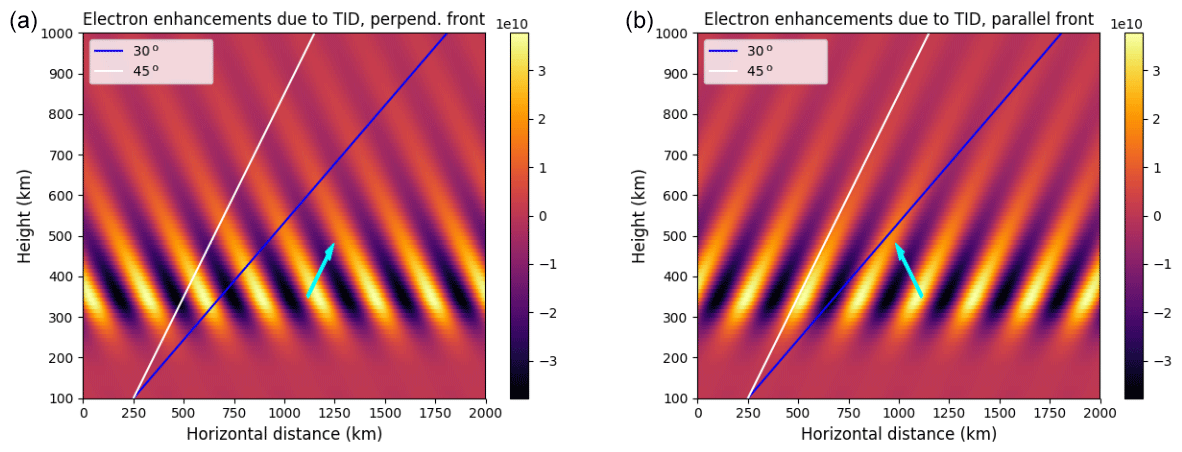
Figure 5Model of electron enhancements due to TIDs. (a) The TID-phase front has been tilted 45∘ to the left. Radar look directions for 45 and 30∘ above the horizon are shown. (b) The same as the plot on the left but with the TID-phase front tilted 45∘ to the right. Both are in units of electrons per cubic meter. The TID wave vector is displayed as a cyan arrow.
In order to evaluate ionospheric blurring of inverse synthetic aperture radar images, we have evaluated different relative look angles between the TID-phase front and the radio wave propagation direction. Angles between 0 and 90∘ with 15∘ steps were considered. Figure 5 shows the fluctuating component of the electron density associated with the TID model for different look angles. The left panel of Fig. 5 shows the best-case scenario, where the radar look direction is perpendicular to the phase front (90∘), and the right panel shows the worst-case scenario, where they are parallel (0∘). We have chosen to use an elevation angle of 45∘ for all cases, as this is close to the value of the highest elevation angle that the Moon can be observed from when using the EISCAT 3D radar. For the model calculations, we used TIDs with a wavelength of 200 km and a period of 10 min. The amplitudes are varied from 1 %–10 % (α=0.01 to α=0.1. For all model calculations, we have assumed a nighttime electron density profile N0(z) based in the International Reference Ionosphere (Bilitza, 2001). We have scaled this electron density profile by a constant value in order to obtain a certain vertical total electron content, as follows:
where L is a vertical path through the ionosphere. We have evaluated the model for vertical total electron content (TEC) of 10 and 40, with units of 1016 electrons per square meter (TECu), corresponding to a low and high ionospheric electron density.
We find that the Doppler broadening depends on (1) the amplitude of TEC enhancement, (2) the background TEC value, and (3) the relative look angle. This is expected since a relative modulation will have a larger effect on the absolute total variation when the background density is higher. With larger look angles, the effect of ionospheric electron density fluctuations average out more and result in smaller ionospheric phase variations.
Table 2Effect of TIDs on Doppler broadening under various conditions.
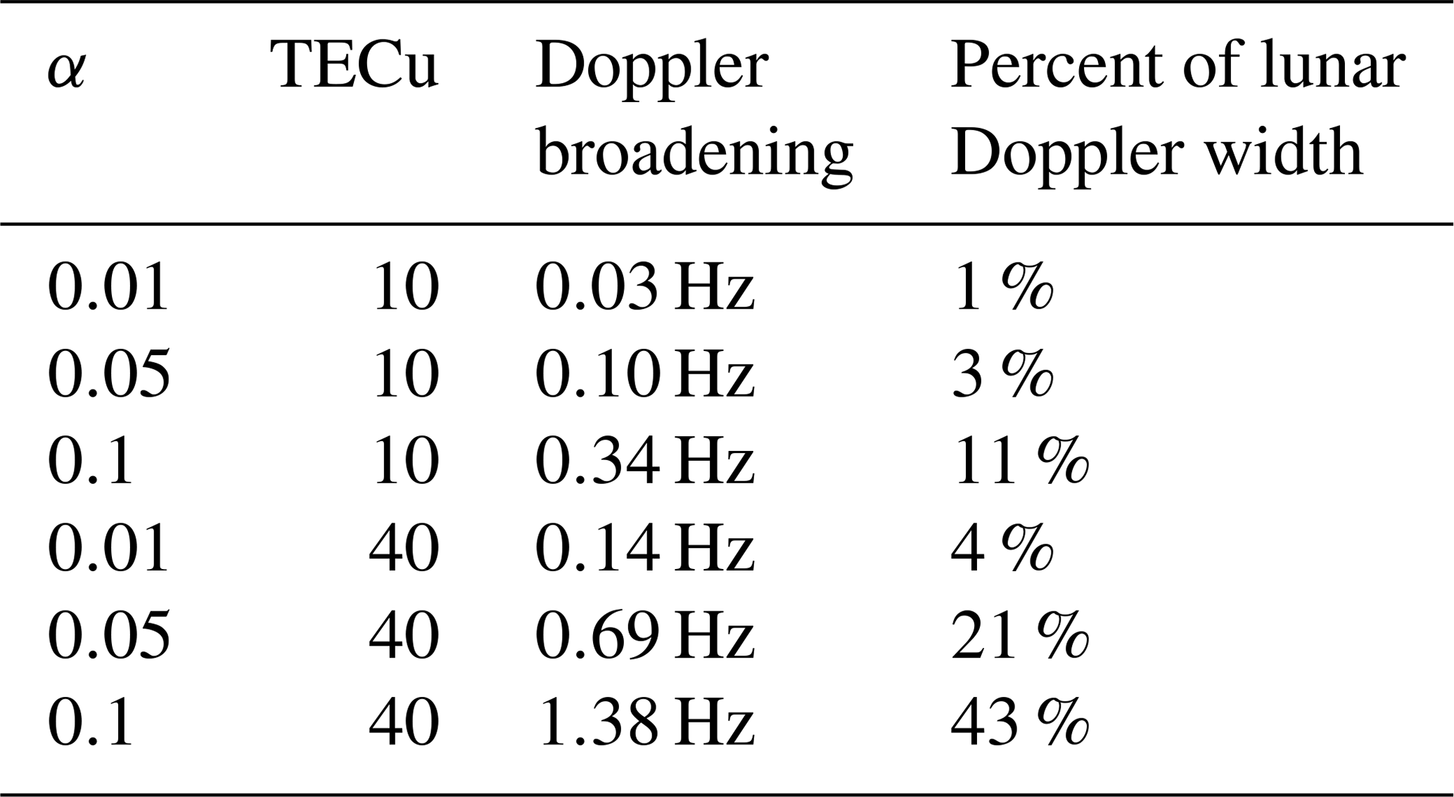
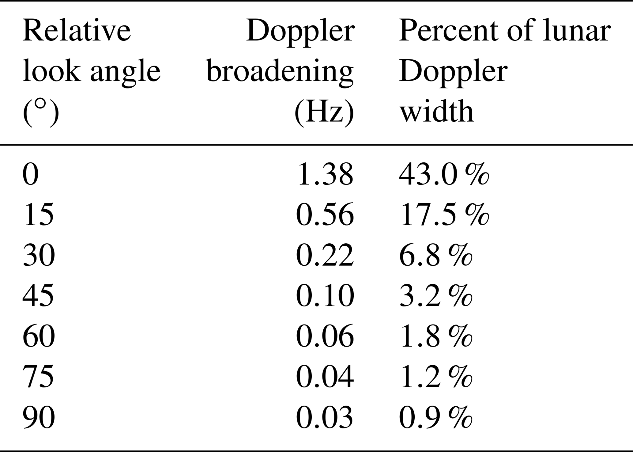
Table 3Effect of the angle between the phase plane and the radar look direction on Doppler broadening, with α=0.1, and TECu is equal to 40.
In Table 2, we have compiled estimates of the ionospheric Doppler broadening caused by a TID where the radar look direction is in the phase plane, which corresponds to the worst case scenario (look angle – 0∘). We have assumed a lunar Doppler width of 3.2 Hz, which would be a typical Doppler width for observations in 2022. The ionospheric Doppler broadening is approximately linear, with both TEC and TID electron enhancement amplitude.

Figure 6All dates on which the lunar face is more than 30∘ over the horizon during 2022, as viewed from the EISCAT 3D Skibotn site. Note that each spike is a lunar month, and every lunar month has several days on which observations are possible.

Figure 7Lunar observation opportunities for 2022–2030. The position of the sub-radar point in selenographic coordinates is shown in light gray. All sub-radar point positions for which the Moon is above 30∘ elevation are shown in green. Each year offers a slightly different view of the Moon.

Figure 8Lunar observation opportunities for 2031–2039. This figure is the same as Fig. 6 but extended further into the 2030s.
In Table 3 we have compiled estimates of frequency distortions of a two-dimensional plane wave TID, with an electron enhancement of 10 %, on a background ionosphere of approximately 40 TECu. In this simulation, we have assumed a radar elevation angle of 45∘. In order to evaluate the impact of changes in the angle between the TID-phase plane and the radar look angle, we changed the tilt of the TID-phase plane from what is shown in the left panel of Fig. 5 to the right panel in 15∘ steps. We can see that the angle to the phase plane is of critical importance for the effect of the phase disruption. When the signal travels through multiple waves, the time dependence of the total electron content is drastically reduced.
The Doppler broadening effects of TIDs are highly variable and can go from negligible to almost as large as the rotational Doppler shift. This is effect is largest when the angle between the radar look direction and the TID-phase plane becomes small. These simple model calculations are representative of what can be expected. Furthermore, previous studies of ionospheric TIDs from Tromsø indicate that conducting the experiment during post-midnight hours in geomagnetically quiet periods is preferable in order to reduce the Doppler broadening effects caused by the ionosphere (Brekke, 2012). Moreover, EISCAT 3D can be used to accurately measure the ionospheric electron density during observations, which can then be used to correct for phase variations caused by the ionosphere.
In order to aid the planning of future lunar observations with EISCAT 3D, we have compiled the possible observation opportunities of the lunar face from the year 2022 to the year 2040. Observation opportunities are plentiful but vary significantly from year to year when it comes to the location of the sub-radar point, Doppler width, and the orientation of the Doppler equator.
Figure 6 is a plot of the lunar elevation in 10 min increments in the year 2022, which is when the EISCAT 3D facility is scheduled for completion. As the facility can steer 60∘ off zenith, there are several days every month that are suitable for lunar observation. Note that each spike consists of several days (∼ 10), with observation opportunities several hours long for most days. The elevation charts of other years are relatively similar. The maximum elevation varies slightly as the orbit of the Moon varies, but this variation does not significantly impact the frequency or duration of observation opportunities.
Figures 7 and 8 show the sub-radar point in selenographic coordinates from the year 2022 up to year 2040. The line is green when the lunar face is at least 30∘ over the horizon, as seen from EISCAT 3D in Skibotn. Over this period, the sub-radar point migrates around the origin of the selenographic coordinate system. Due to this migration, the view of the lunar nearside changes as the horizons and rotation direction change. The mid-2020s will provide a view of the lunar south pole, while the mid-2030s will allow us to study the northern regions. As the sub-radar point migrates day to day and year to year, some regions near the lunar limbs are only visible for a fraction of the time. Care should then be taken to ensure that interesting regions are observed when they are observable, as opportunities do not repeat often.
The range resolution Rr achievable is found as , where B is the transmit bandwidth, and c is the speed of light. As EISCAT 3D has a transmit bandwidth of 5 MHz, this results in a range resolution along sight of approximately 30 m. The frequency resolution Rf along the equator is found as , where Dm is the diameter of the Moon, vrot, and τm is the observation time in seconds. The apparent rotation velocity of the Moon will change day to day but will be somewhere between 0.5 and 2.0 m s−1. For a 1 h observation with an apparent rotation velocity of 1.2 m s−1, the average resolution in the Doppler dimension will be 520 m.
The practically achievable resolution will be significantly lower than what is theoretically possible. Much of this reduction comes from efforts to compensate for low SNR and to reduce speckling. Another challenge is that the Rogers and Ingalls method of north–south disambiguation assumes a stationary Doppler axis. This assumption does not hold for long observations of the lunar face, effectively limiting possible observation times. These effects will be dependent upon the specifics of each observation and can be expected to vary significantly.
EISCAT 3D provides an excellent new tool for radar imaging of the lunar nearside. Observation opportunities are plentiful and varied, and the radar can track the lunar face for sufficiently long periods of time to allow high-quality observations to be made. The operating frequency of EISCAT 3D is previously unused for lunar mapping purposes and will, therefore, provide new information about the scattering properties of the lunar terrain. The interferometric capabilities provided by the large number of receiving antennae are able to resolve the north–south ambiguity, even close to the Doppler equator. This means that it will take fewer unique looks to obtain a full coverage map of the lunar nearside.
The other terrestrial planets are too far away for EISCAT 3D to achieve a scientifically useful resolution due to the low signal strength. This could possibly be rectified by increasing the transmitted power and/or receiver gain function of the facility some time in the future, though this may be unrealistic in practice.
The ability of the radar facility to track moving targets and steer down to 30∘ elevation allows for many long observation opportunities. This will be useful for mitigating the disrupting effects of ionospheric variability, as experiments can easily be rescheduled. TIDs can be a significant hindrance to obtaining clear radar images, but the most disruptive events should not be very common.
The variability in the lunar sub-radar point and Doppler axis will allow for varied views of the lunar face. Regular observations over the course of several years can provide new views of regions that are occasionally obscured by the lunar horizon.
This article provides an expansion of the science case for EISCAT 3D into the realm of planetary radar mapping. While NEOs can also fall under the umbrella term of planetary radar, this science case is discussed in detail in the companion paper by Kastinen et al. (2020), which also appears in this special issue.
The source code is provided by a GitHub repository via Zenodo (https://doi.org/10.5281/zenodo.4740248; Tveito and Vierinen, 2021).
The data set used in this paper is available upon request.
TT performed numerical calculations for the TID simulations, interferometric disambiguation, and ionospheric frequency disturbances. JV performed the compilation of observation opportunities and signal-to-noise ratio calculations of planetary targets. BG contributed to the calculation of observation opportunities, interferometric disambiguation, and TID simulation. VLN contributed to Sect. 5, for both the calculation and interpretation of the results. All authors contributed to the writing of the paper and the interpretation of results.
Juha Vierinen is on the editorial board of this special issue.
This article is part of “Special Issue on the joint 19th International EISCAT Symposium and 46th Annual European Meeting on Atmospheric Studies by Optical Methods”. It is a result of the 19th International EISCAT Symposium 2019 and 46th Annual European Meeting on Atmospheric Studies by Optical Methods, Oulu, Finland, 19–23 August 2019.
Torbjørn Tveito and Juha Vierinen would like to thank the Tromsø Research Foundation for supporting this work.
This research has been supported by the Tromsø research foundation (Project: Radar science with EISCAT 3D).
This paper was edited by Andrew J. Kavanagh and reviewed by Sriram Bhiravarasu and one anonymous referee.
Bilitza, D.: International reference ionosphere 2000, Radio Sci., 36, 261–275, 2001. a
Bolmgren, K., Mitchell, C., Bruno, J., and Bust, G.: Tomographic Imaging of Traveling Ionospheric Disturbances Using GNSS and Geostationary Satellite Observations, J. Geophys. Res.-Space, 125, e2019JA027, https://doi.org/10.1029/2019JA027551, 2020. a
Brekke, A.: Physics of the upper polar atmosphere, Springer Science & Business Media, Heidelberg, 2012. a
Busch, M. W., Kulkarni, S. R., Brisken, W., Ostro, S. J., Benner, L. A., Giorgini, J. D., and Nolan, M. C.: Determining asteroid spin states using radar speckles, Icarus, 209, 535–541, 2010. a
Campbell, B. A.: Radar remote sensing of planetary surfaces, Cambridge University Press, Cambridge, 2002. a
Campbell, B. A.: Planetary geology with imaging radar: insights from earth-based lunar studies, 2001–2015, Publ. Astron. Soc. Pac., 128, 062001, https://doi.org/10.1088/1538-3873/128/964/062001, 2016. a, b
Campbell, B. A., Campbell, D. B., Margot, J.-L., Ghent, R. R., Nolan, M., Chandler, J., Carter, L. M., and Stacy, N. J.: Focused 70-cm wavelength radar mapping of the Moon, IEEE T. Geosci. Remote Sens., 45, 4032–4042, 2007. a
Campbell, B. A., Campbell, D. B., Carter, L. M., Chandler, J. F., Giorgini, J. D., Margot, J.-L., Morgan, G. A., Nolan, M. C., Perillat, P. J., and Whitten, J. L.: The mean rotation rate of Venus from 29 years of Earth-based radar observations, Icarus, 332, 19–23, 2019. a
Davies, K.: Ionospheric radio propagation, Vol. 80, US Department of Commerce, National Bureau of Standards, Washington, DC, 1965. a
Evans, J. V. and Hagfors, T.: Radar astronomy, raas, edited by: Evans, J. V. and Hagfors, T., McGraw-Hill, New York, 1968. a
Giorgini, J., Chodas, P., and Yeomans, D.: Orbit uncertainty and close-approach analysis capabilities of the horizons on-line ephemeris system, in: DPS, Vol. 33, 58–13, 2001. a
Giorgini, J. D., Benner, L. A., Ostro, S. J., Nolan, M. C., and Busch, M. W.: Predicting the Earth encounters of (99942) Apophis, Icarus, 193, 1–19, 2008. a
Goldstein, R. and Carpenter, R.: Rotation of Venus: Period estimated from radar measurements, Science, 139, 910–911, 1963. a
Harmon, J. K., Slade, M. A., and Rice, M. S.: Radar imagery of Mercury’s putative polar ice: 1999–2005 Arecibo results, Icarus, 211, 37–50, 2011. a
Kastinen, D., Tveito, T., Vierinen, J., and Granvik, M.: Radar observability of near-Earth objects using EISCAT 3D, Ann. Geophys., 38, 861–879, https://doi.org/10.5194/angeo-38-861-2020, 2020. a, b, c, d
Kero, J., Kastinen, D., Vierinen, J., Grydeland, T., Heinselman, C. J., Markkanen, J., and Tjulin, A.: EISCAT 3D: the next generation international atmosphere and geospace research radar, Proceedings of the first NEO and Debris Detection Conference, edited by: Flohrer, T., Jehn, R., and Schmitz, F., ESA Space Safety Programme Office, Darmstadt, 2019. a
Margot, J.-L., Campbell, D. B., Jurgens, R. F., and Slade, M. A.: Digital elevation models of the Moon from Earth-based radar interferometry, IEEE T. Geosci. Remote Sens., 38, 1122–1133, 2000. a
McCrea, I., Aikio, A., Alfonsi, L., Belova, E., Buchert, S., Clilverd, M., Engler, N., Gustavsson, B., Heinselman, C., Kero, J., Kosch, M., Lamy, H., Leyser, T., Ogawa, Y., Oksavik, K., Wannberg, A., Pitout, F., Rapp, M., Stanislawska, I., and Vierinen, J.: The science case for the EISCAT_3D radar, Prog. Earth Pl. Sci., 2, 1–63, 2015. a
Ostro, S. J.: Planetary radar astronomy, Rev. Modern Phys., 65, 1235, https://doi.org/10.1103/RevModPhys.65.1235, 1993. a, b, c
Phillips, R. J., Raubertas, R. F., Arvidson, R. E., Sarkar, I. C., Herrick, R. R., Izenberg, N., and Grimm, R. E.: Impact craters and Venus resurfacing history, J. Geophys. Res.-Pl., 97, 15923–15948, 1992. a
Rogers, A. and Ingalls, R.: Venus: Mapping the surface reflectivity by radar interferometry, Science, 165, 797–799, 1969. a, b
Shalygin, E., Basilevsky, A., Markiewicz, W., Titov, D., Kreslavsky, M., and Roatsch, T.: Search for ongoing volcanic activity on Venus: Case study of Maat Mons, Sapas Mons and Ozza Mons volcanoes, Planet. Space Sci., 73, 294–301, 2012. a
Shiokawa, K., Mori, M., Otsuka, Y., Oyama, S., Nozawa, S., Suzuki, S., and Connors, M.: Observation of nighttime medium-scale travelling ionospheric disturbances by two 630-nm airglow imagers near the auroral zone, J. Atmos. Solar-Terr. Phys., 103, 184–194, 2013. a, b
Spudis, P., Bussey, D., Baloga, S., Cahill, J., Glaze, L., Patterson, G., Raney, R., Thompson, T., Thomson, B., and Ustinov, E.: Evidence for water ice on the Moon: Results for anomalous polar craters from the LRO Mini-RF imaging radar, J. Geophys. Res.-Pl., 118, 2016–2029, 2013. a
Stamm, J., Vierinen, J., Urco, J. M., Gustavsson, B., and Chau, J. L.: Radar imaging with EISCAT 3D, Ann. Geophys., 39, 119–134, https://doi.org/10.5194/angeo-39-119-2021, 2021. a
Thompson, T.: A review of Earth-based radar mapping of the Moon, Moon Planets, 20, 179–198, 1979. a
Thompson, T. W.: High resolution lunar radar map at 7.5 meter wavelength, Icarus, 36, 174–188, 1978. a
Thompson, T. W., Campbell, B. A., Ghent, R. R., Hawke, B. R., and Leverington, D. W.: Radar probing of planetary regoliths: An example from the northern rim of Imbrium basin, J. Geophys. Res.-Pl., 111, E06S14, https://doi.org/10.1029/2005JE002566, 2006. a
Tveito, T. and Vierinen, J.: TorbjornTveito/E3D-planetary-science: E3D-planetary-science, Zenodo [Dataset], https://doi.org/10.5281/zenodo.4740248, 2021.
Vierinen, J.: Beacon satellite receiver software for ionospheric tomography, Radio Sci., 49, 1141–1152, 2011. a
Vierinen, J., Markkanen, J., Krag, H., Siminski, J., and Mancas, A.: Use of EISCAT 3D for Observations of Space Debris, ESA Space Debris Office, 2017a. a
Vierinen, J., Tveito, T., Gustavsson, B., Kesaraju, S., and Milla, M.: Radar images of the Moon at 6-meter wavelength, Icarus, 297, 179–188, 2017b. a, b, c, d, e, f, g, h
- Abstract
- Introduction
- EISCAT 3D
- Detectability of planetary bodies
- Range–Doppler disambiguation
- Ionospheric effects
- Future lunar observation opportunities
- Conclusions
- Code availability
- Data availability
- Author contributions
- Competing interests
- Special issue statement
- Acknowledgements
- Financial support
- Review statement
- References