the Creative Commons Attribution 4.0 License.
the Creative Commons Attribution 4.0 License.
 | 01 Apr 2021
Temperature decadal trends, and their relation to diurnal variations in the lower thermosphere, stratosphere, and mesosphere, based on measurements from SABER on TIMED
Frank T. Huang
Hans G. Mayr
We have derived the behavior of decadal temperature trends over the 24 h of local time, based on zonal averages of SABER data, for the years 2012 to 2014, from 20 to 100 km, within 48∘ of the Equator. Similar results have not been available previously. We find that the temperature trends, based on zonal mean measurements at a fixed local time, can be different from those based on measurements made at a different fixed local time. The trends can vary significantly in local time, even from hour to hour. This agrees with some findings based on nighttime lidar measurements. This knowledge is relevant because the large majority of temperature measurements, especially in the stratosphere, are made by instruments on sun-synchronous operational satellites which measure at only one or two fixed local times, for the duration of their missions. In these cases, the zonal mean trends derived from various satellite data are tied to the specific local times at which each instrument samples the data, and the trends are then also biased by the local time. Consequently, care is needed in comparing trends based on various measurements with each other, unless the data are all measured at the same local time. Similar caution is needed when comparing with models, since the zonal means from 3D models reflect averages over both longitude and the 24 h of local time. Consideration is also needed in merging data from various sources to produce generic, continuous, longer-term records. Diurnal variations of temperature themselves, in the form of thermal tides, are well known and are due to absorption of solar radiation. We find that at least part of the reason that temperature trends are different for different local times is that the amplitudes and phases of the tides themselves follow trends over the same time span of the data. Many of the past efforts have focused on the temperature values with local time when merging data from various sources and on the effect of unintended satellite orbital drifts, which result in drifting local times at which the temperatures are measured. However, the effect of local time on trends has not been well researched. We also derive estimates of trends by simulating the drift of local time due to drifting orbits. Our comparisons with results found by others (Advanced Microwave Sounding Unit, AMSU; lidar) are favorable and informative. They may explain, at least in part, the bridge between results based on daytime AMSU data and nighttime lidar measurements. However, these examples do not form a pattern, and more comparisons and study are needed.
- Article
(5870 KB) - Full-text XML
- BibTeX
- EndNote


The understanding of decadal temperature trends in the middle and upper atmosphere is interesting scientifically and important for practical reasons. Global temperature trends have been researched for decades based on a variety of satellite and ground-based measurements. However, relatively few studies have focused on the behavior of trends as a function of local time. Past efforts have focused more on the local time variations of temperature themselves in comparing or merging various data sets and on accounting for drifts in local time of measurements due to satellite orbital stability.
Diurnal variations of temperatures themselves, in the form of thermal tides, are well known and are a result of absorption of solar radiation (see Brasseur and Solomon, 2005, and references therein).
Understanding the behavior of trends with local time can be important because the large majority of global temperature measurements, especially in the stratosphere, are made by sun-synchronous satellites whose instruments measure temperature at only one or two fixed local times, for the duration of their missions. In these cases, the zonal mean trends derived from various satellite data are tied to and biased by the specific local times at which each instrument samples the data.
Care is then needed in comparing results of trends derived from various measurements which sample data at different local times. It is also needed when merging data from various sources to produce generic, continuous, longer-term records. In addition, the zonal means of 3D models are averages of temperatures over both longitude and the 24 h of local time, and comparisons with trends based on data taken at fixed local times, or a subset of local times, can be problematic (Austin et al., 2008).
In the following, based on data from the Sounding of the Atmosphere using Broadband Emission Radiometry (SABER) instrument on the Thermosphere Ionosphere Mesosphere Energetics and Dynamics (TIMED) satellite, we derive the local-time dependence of decadal temperature trends over the 24 h of local time, from 2002 to 2014, from the stratosphere into the lower thermosphere (20 to 100 km), within 48∘ of the Equator.
Comparable results for temperature trends have not been available previously.
Our starting point here is based on results from our past studies, also based on SABER data. Previously, we have estimated diurnal variations of the temperature (thermal tides) for each day, expressed in the form of five Fourier series components (Huang et al., 2010a). We have also derived zonal means of temperature that are averages over both longitude and local time for a latitude circle (Huang et al., 2006, 2010a). These “synoptic” zonal means are important because they can then be compared directly with 3D models. Details are given in Sect. 2.
Using these past results, here we derive the behavior of decadal temperature trends as a function of local time.
We find that the temperature trends, based on zonal mean measurements at a fixed local time, can be different from those based on measurements made at a different fixed local time. These variations of trends can be significant in all regions of our study and can vary significantly, even from hour to hour.
Our results suggest that part of the reason that temperature trends are different for different local times is that the tidal amplitudes and phases of the tides also follow trends over the time span of the data.
In the following, we compare trends with results of trends by others. Because trends vary with the time span considered, comparisons should cover similar times, and the opportunities are limited.
Although the comparisons support our results of local time variations in trends, more comparisons are needed.
Global stratospheric data are largely from the NOAA series of operational satellites and the Earth Observing System of satellites. These are generally in sun-synchronous orbits, so that data are sampled at only one or two local times, which are fixed for the duration of the missions. The operational satellites are meant in part to monitor the atmosphere over the longer term and have been making measurements since the 1970s. Over the years, they are replaced as needed, in order to maintain a continuous record of data. However, there have been issues of data continuity and compatibility among the different satellites, related to data sampling, instrument calibration, and operation. Also, over the years, the orbits of some satellites have drifted from their planned sun-synchronous state, so that the local times at which the measurements are made have also drifted over several hours or more.
There have been group and individual efforts to combine and merge the data from different sources to obtain uniform, consistent, decades-long databases for temperature (and others). Some of the issues are concerned with differences due to local times when merging data. For example, Mears and Wentz (2016) have considered the sensitivity of temperature trends to “diurnal cycle adjustment” and improved the consistencies of the different data sets caused by orbital drifts in local time, based on cross-information from other satellites and on general circulation models. Keckut et al. (2015) have also shown that considering atmospheric tides to account for differences among measurements of successive operational polar orbiting satellites would improve matters. Funatsu et al. (2008) have studied the differences among nighttime lidar data and daytime sun-synchronous satellite data. Randel et al. (2016), McLandress et al. (2015), and Zou et al. (2014), among others, have also considered the issue of merged data from various sources, with consideration for differences due to effects of local time
These merged long-term data sets have general advantages of providing data for studies of trends and responses to solar activity. However, as noted earlier, if the various data sets do not represent uniform sampling in local time, the merged data could be tagged by the biases in local time.
Because we make use of our previous results of temperature diurnal variations and trends, we briefly review them for the convenience of the reader. Our previous results on temperature trends were based only on zonal means that are averages over both longitude and local time. See Huang et al. (2014, 2010a).
The SABER instrument was launched in December 2001 on the TIMED satellite (Russell et al., 1999). The data used here are version 2.0, level 2A. The values are interpolated to 4∘ latitude and 2.5 km altitude grids, and zonal averages are taken for analysis.
SABER temperature measurements have been analyzed with success by us and by others.
Zhang et al. (2006) and Mukhtarov et al. (2009) have derived temperature diurnal tides using SABER data, and Nath and Sridharan (2014) have derived temperature trends using the same SABER data but without accounting for diurnal variations. We have derived variations with periods from less than 1 d (diurnal variations) up to multiple years (semiannual oscillation, SAO; quasi-biennial oscillation, QBO), and 1 decade or more (responses to the solar cycle). See Huang et al. (2010a, 2014, 2016a, b).
In a previous paper, Huang and Mayr (2019) also analyzed the effects of local time on the response of temperature (and ozone) to the solar cycle (∼ 11 years).
2.1 Diurnal variations
Due to the orbital characteristics of TIMED, SABER measurements provide the potential to estimate the variations of temperature as a function of the 24 h of local time that data from other satellites generally do not provide. The local times of the SABER measurements decrease by about 12 min from day to day, and it takes 60 d to sample over the 24 h of local time, using both ascending- and descending-node data. Although this provides essential information over the range of local times, over 60 d, variations can be due to both local time and other variables, such as season. Diurnal and mean variations are embedded together in the data and need to be unraveled from each other to obtain more accurate estimates of each.
Our algorithm is designed for this type of sampling in local time and provides estimates of both diurnal and mean (e.g., annual, semiannual, and seasonal oscillations) variations together in a consistent manner. At a given latitude and altitude for zonal mean data over a period of a year, the algorithm performs a least-squares estimate of a two-dimensional Fourier series, where the independent variables are local time and day of year, and variations as a function of local time and day of year are generated.
The fundamental Fourier period in day of year is 365 d, and that for local time is 24 h. For subsequent months and years, the initial analysis serves as a sliding data window. To find subsequent monthly values, this window is advanced by 1 month, and the algorithm is applied again. Further details can be found in Huang et al. (2010a).
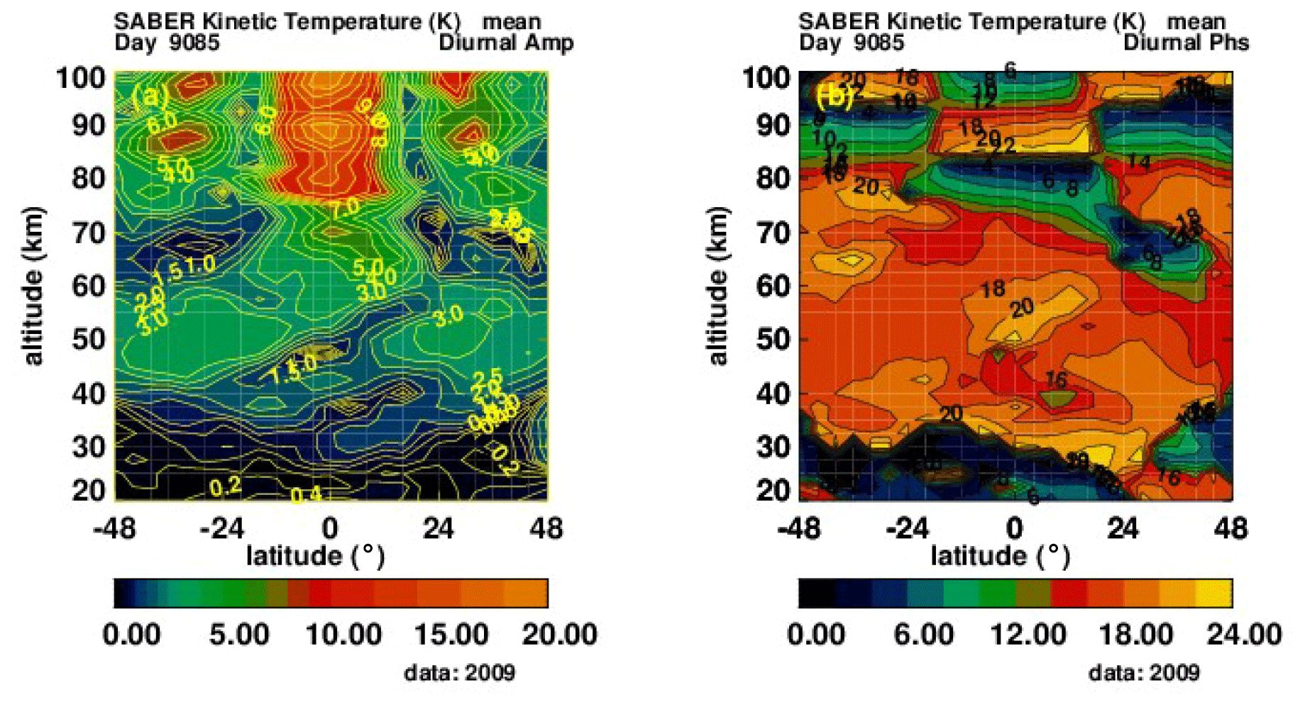
Figure 1Temperature tides from 20 to 100 km, 48∘ S to 48∘ N, day 85, year 2009. (a) Diurnal amplitudes (K). (b) Diurnal phases (h of maximum value).
Figure 1 shows an example of temperature diurnal amplitudes (Fig. 1a) and phases (Fig. 1b) of the diurnal tide on altitude–latitude coordinates (20 to 100 km, 48∘ S to 48∘ N), for day 85 of 2009. Although not shown, higher components, such as the semidiurnal tides, can also be significant. Our derivation includes five Fourier components.
2.2 Mean variations
The zonal mean variations, which are averages over both longitude and local time, consistent with 3D models, are obtained together with the diurnal variations.
Based on these zonal means, our earlier results of trends and decadal responses to solar activity were presented in Huang et al. (2014, 2016a, b, 2019).
For the current analysis, we use the diurnal and mean variations together and generate zonal means at any selected local time.
In the following, we generate
-
monthly zonal means that are averages over longitude, but at specific local times, that correspond to measurements by sun-synchronous satellites and nighttime lidar measurements;
-
monthly zonal means to simulate satellite orbital drifts, with local times that vary from month to month;
-
monthly zonal means that are averages over longitude and the 24 h of local time, as previously done.
From (1), (2), and (3) we estimate temperature trends using Eq. (1), in a similar manner as previously done by others, and by us, using a multiple regression analysis that includes solar activity, trends, seasonal, quasi-biennial oscillation (QBO), and local time terms, on monthly values. Specifically, the estimates are found from the following equation:
where t is time (months), a is a constant, b is the trend, d the coefficient for solar activity (10.7 cm flux), c is the coefficient for the seasonal (S(t)) variations, l is the coefficient for local time (lst) variations, and g is the coefficient for the QBO. As is often done, the seasonal and local time variations are removed first, but we include them in Eq. (1) for completeness. F10.7 stands for the solar 10.7 cm flux, which is commonly used as a measure of solar activity, and the values used here are monthly means provided by NOAA.
T stands for the various input temperature zonal means described in (1), (2), and (3) above.
The multiple regression is applied to the monthly zonal-mean values from June 2002 through June 2014, from 48∘ S to 48∘ N latitude, and from 20 to 100 km.
The analysis of uncertainties is the same for this study as for the previous study of the mean variations just described. Here the zonal means are generated at specific local times. Details and results of the statistical analysis are given in Huang et al. (2014, 2106a).
Before presenting our overall trend results as a function of local time, we first compare some specific results with those by others. The merged data sets noted earlier do not represent uniform averages over the range of local times, nor do they represent specific fixed local times. In addition, they span a longer time interval than the SABER data, and we will not use them for comparisons. Because trends can significantly depend on the particular time period, comparisons are limited to the time span of ∼ 2002 to 2014.
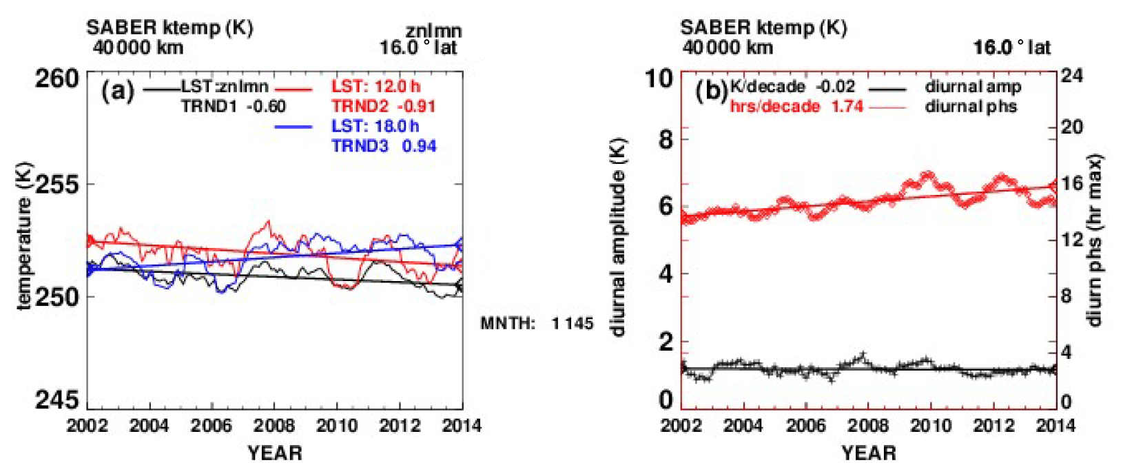
Figure 2(a) Monthly SABER temperature (K) from 2002 to 2014, 40 km, 16∘ N latitude. Black line: zonal mean values (averages over longitude and local time); red line: zonal mean at 12:00 LT; blue line: zonal mean at 18:00 LT. (b) On the left axis scale, black line: tidal diurnal amplitude (K). On the right axis scale, red line: diurnal phase (h of maximum value).
Figure 2a shows examples of our estimates of monthly SABER values of temperature (K) from mid-2002 to mid-2014, without the diurnal and seasonal variations. The black line shows zonal mean values that are averages over both longitude and local time at 40 km and 16∘ latitude, with a trend of ∼ −0.6 K per decade, found from a linear fit. The red line shows monthly values of zonal means at a fixed 12:00 LT, with a trend of ∼ −0.91 K per decade. The blue line represents monthly values of zonal means at a fixed local time of 18:00 LT, with a trend of ∼ +0.94 K per decade. Figure 2b shows the temperature tidal diurnal amplitude (black line, left-hand scale) and the diurnal phase (red line, hour of maximum value, right-hand scale).
The trends of the diurnal amplitudes and phases themselves contribute to the different temperature trends at different local times. Although not shown, we note that semidiurnal tides are not negligible. Additional plots corresponding to Fig. 2b are given in the Appendix.
4.1 Stratosphere
For the stratosphere, we compare with trends given by Funatsu et al. (2016), based on data from the Advanced Microwave Sounding Unit (AMSU) on the NASA Aqua satellite and from nighttime ground-based lidar measurements. The results of Funatsu et al. (2016) are suitable for comparison because the time span of the data is similar to ours (2002 to 2014), and AMSU samples data near specific local times, namely, 13:30 and 01:30 LT.
Following Funatsu et al. (2016), the AMSU is a cross-scanning microwave-based sounder, and the channels 9–14 sample with weighting functions peaking at approximately 18, 20, 25, 30, 35, and 40 km. The horizontal resolution at the near-nadir field of view is approximately 48 km, and the vertical half width of the weighting functions is about 10 km.
Although the lidar measurements presented by Funatsu et al. (2016) also cover a similar time span (2002–2013), they are made only during nighttime from the Observatoire de Haute Provence (OHP; 43.91∘ N, 5.71∘ E) and the Mauna Loa Observatory (MLO; 19.51∘ N, 155.61∘ W).
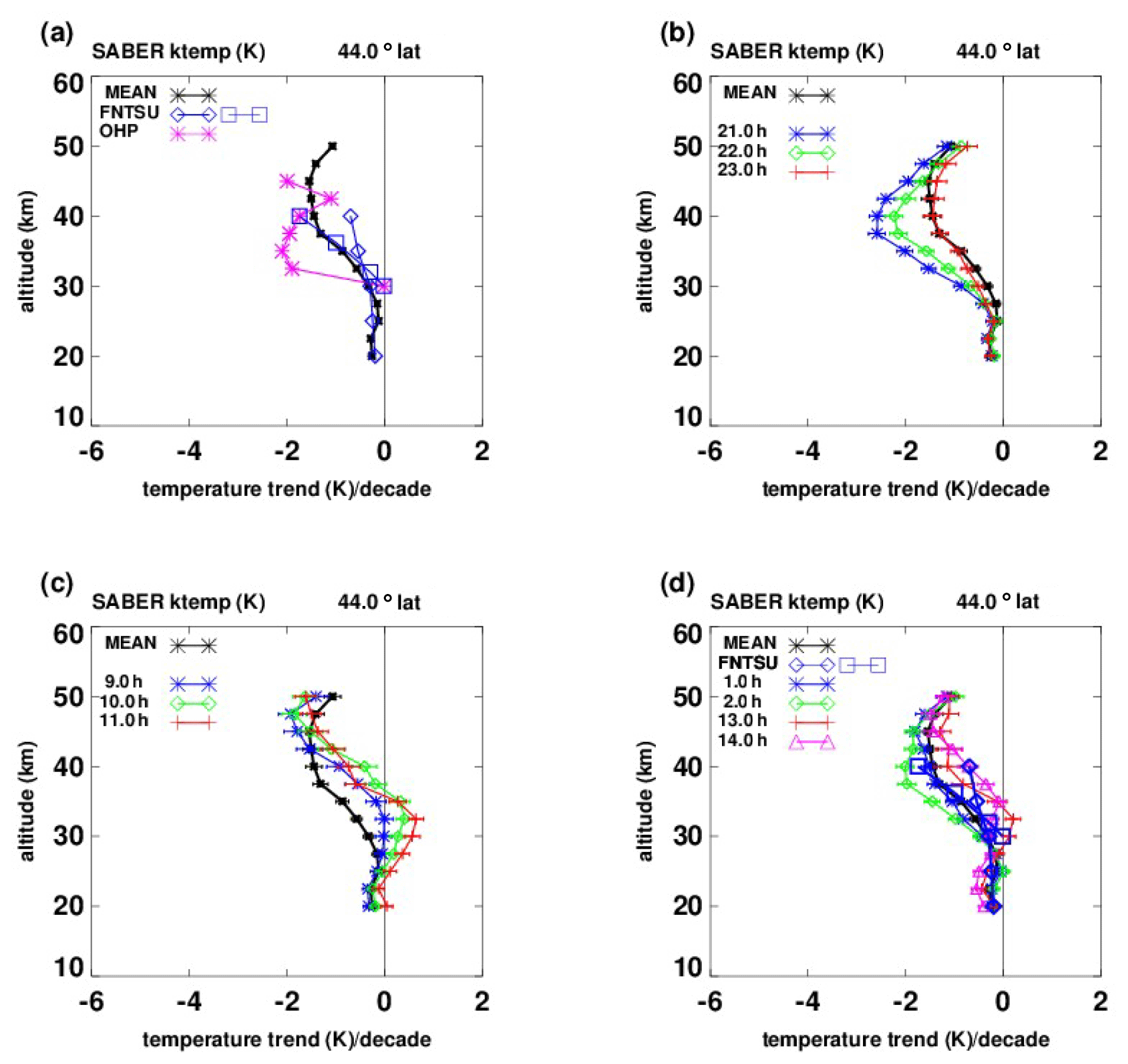
Figure 3Temperature trends (K per decade, 2002–2014) vs. altitude. (a) Black asterisks: based on SABER zonal means (over longitude and local time) at 44∘ N; blue diamonds: Funatsu Aqua trends for midlatitudes (30–60∘ N); blue squares: Funatsu Aqua trends at 44∘ N; magenta asterisks: based on nighttime lidar measurements at OHP (44∘ N). (b) Black asterisks: same as (a), blue, green, red: our estimates at 21:00, 22:00, 23:00 LT, based on SABER data. (c) Black asterisks: same as (a), blue, green, red: our estimates at 09:00, 10:00, 11:00 LT. (d) Black asterisks, same as (a); blue diamonds and squares: as in (a), Funatsu AMSU, blue asterisks, green diamonds, red plus symbols, magenta triangles: SABER trends at 01:00, 02:00, 13:00, 14:00 LT.
Figure 3 shows our results of temperature trends (K per decade), based on SABER data (2002 to 2014), and those from Funatsu et al. (2016), based on AMSU and lidar measurements. For AMSU, Fanatsu et al. (2016) provide trends as a function of channel numbers for the low-latitude and midlatitude composite trends, so following McLandress et al. (2015), we use the altitudes of the weighting function peaks, namely 20, 25, 30, 35, and 40 km, for comparison. They do provide altitudes in kilometers for comparison with lidar. We note that where the values and altitudes are given by others such as Funatsu et al. (2016), we have transferred them manually to our figures, as needed.
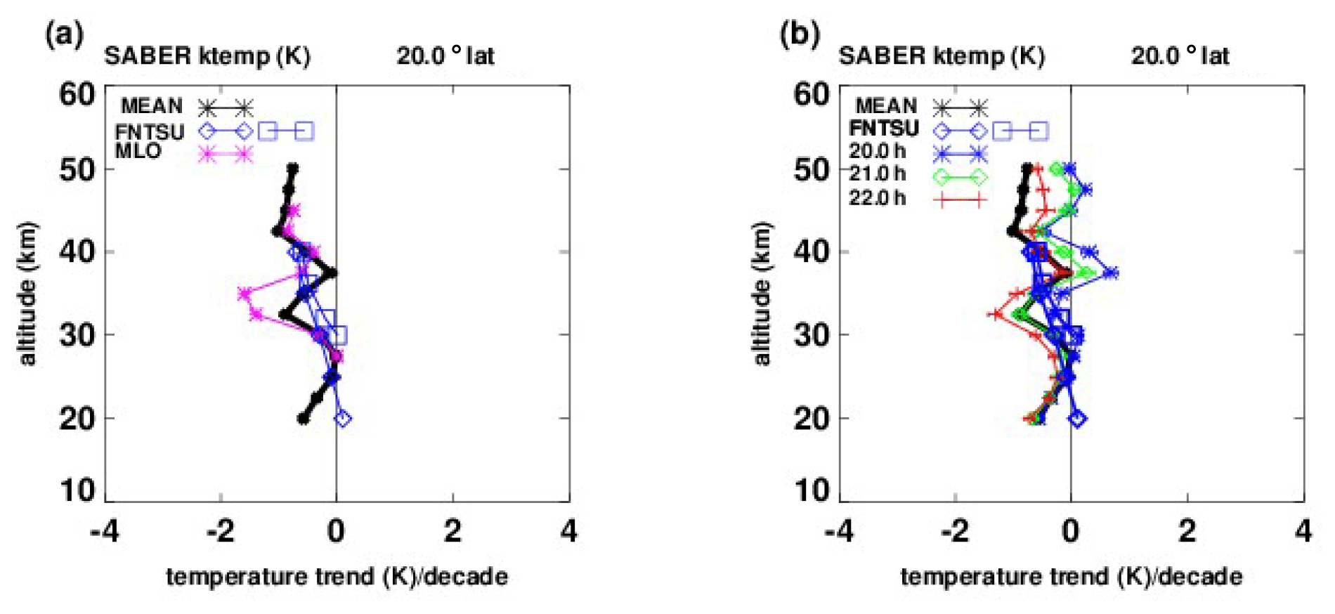
Figure 4Temperature trends (K per decade) vs. altitude. (a) Black asterisks: trends based on SABER zonal means (over longitude and local time) at 20∘ N; blue diamonds: Funatsu et al. (2016) Aqua; data at 13:30 and 01:30, low latitudes (0 to 30∘ N); blue squares: Funatsu Aqua at 20∘ N; magenta asterisks: lidar measurements at Mauna Loa Observatory (MLO, 19.51∘ N), (b) Black asterisks: same as (a), blue, green, red: estimates at 20:00, 21:00, 22:00 LT, based on SABER data.
In Fig. 3a, the black line plots trend results based on SABER zonal means found by averages over both local time and longitude. The blue diamonds and squares are from Funatsu et al. (2016), based on AMSU data, presumably averages taken near 01:30 and 13:30 LT. The blue diamonds denote zonal mean trends for midlatitudes (30 to 60∘ N), and the blue squares represent trends at 44∘ N that correspond to OHP. The blue squares are available only from 30 to 40 km (∼ 30, 32.0, 36.2, 40.0 km) but match our results (black line) at 44∘ N extremely well. The blue diamonds (from Funatsu AMSU, an amalgam to represent midlatitudes) match our results almost exactly from 20 to 30 km but are larger from 30 to 40 km. This could simply be because the blue diamonds represent midlatitudes (30 to 60∘ N), while the blue squares and our black line represent trends at 44∘ N specifically. The magenta asterisks, also provided by Funatsu et al. (2016), based on nighttime lidar measurements at 44∘ N, are significantly more negative from 30 to 40 km than our results and those of the Funatsu et al. (2016) AMSU. Figure 3b shows our nighttime results from SABER at 21:00, 22:00, and 23:00 LT. It can be seen that our nighttime results agree better with the nighttime lidar trends (magenta asterisks) in Fig. 3a. We do not know the details of the nighttime hours of the lidar data. Figure 3c shows our daytime trends at 09:00, 10:00, and 11:00 LT, and these agree less well with the lidar trends.
The average of all our night and daytime trends gives the zonal mean average shown by the black line. Figure 3d compares our results at 01:00, 02:00, 13:00, and 14:00 LT with the AMSU results. They are near the local times of the AMSU data (presumably 01:30 and 13:30:00 LT). It can be seen that the averages over the four local times compare favorably with those of Funatsu et al. (2016), based on AMSU data. It is not clear if Funatsu et al. (2016) differentiated night from day measurements.
We believe that, by taking into account trends with local time, our results compare favorably with both the Funatsu et al. (2016) AMSU trends and their results based on nighttime lidar data.
Figure 4a corresponds to Fig. 3a but for 20∘ N to compare with results of Funatsu et al. (2016) based on AMSU low-latitude and nighttime lidar results at the Hawaiian Mauna Loa Observatory (MLO, 19.51∘ N). As in Fig. 3 for OHP, the lidar results show a diversion to more negative trends near 30–35 km. Here, our results, as represented by trends based on zonal means that are averages over local time, also show a decrease, although not as pronounced, near 30–35 km. As in Fig. 3, both the blue diamonds and blue squares are from Funatsu et al. (2016) based on AMSU data but for low latitudes (0 to 30∘ N) and 20∘ N latitude respectively. They are smoother than our results between 25 and 40 km and do not show the notch near 30 km that our trends and the lidar-based trends show. This could be due to the differences in altitude resolution between AMSU and lidar and SABER data.
As can be seen in Fig. 4b, the decrease on our trends near 30 km is due in large part to the behavior at 21:00 and 22:00 LT (green diamonds, red plus symbols).
Figures 3 and 4 show that by taking into account the different trends with local time, our results compare more favorably with those of the Funatsu et al. (2016), based on AMSU and lidar data. Figures 3 and 4 also show that trends can change significantly with local time, even from hour to hour.
However, our comparisons do not form a pattern, and more comparisons are of course needed.
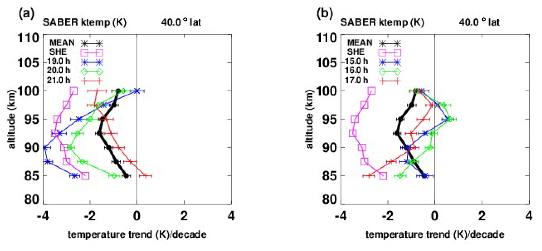
Figure 5Temperature trends (K per decade) vs. altitude, at 40∘ N latitude. (a) Black asterisks: trends based on SABER zonal mean (over longitude and local time); blue asterisks, green diamonds, red plus symbols: trends based on SABER zonal means at 19:00, 20:00, 21:00 LT. Magenta squares: trends based on nighttime lidar measurements by She et al. (2019); (b) as in (a) but for SABER results at 15:00, 16:00, 17:00 LT.
We note that the results of Khaykin et al. (2017) based on analysis of GPS radio occultation (GRO) measurements are in excellent agreement with AMSU (based on a slightly longer period (2002–2016). Khaykin et al. (2017) state that “after down sampling of GRO profiles according to the AMSU weighting functions, the spatially and seasonally resolved trends from the two data sets are in almost exact agreement with trends based on AMSU data.”
4.2 Lower thermosphere
In Fig. 5, we compare our results (K per decade) with the lidar nighttime measurements of She et al. (2019), at Fort Collins, CO (41∘ N, 105∘ W), and Logan, UT (42∘ N, 112∘ W), from 2002–2014. They actually made nocturnal temperature observations between 1990 and 2017 but divided their analysis into various time periods and smaller time intervals within the nighttime hours. This provides valuable information regarding trends and local time. In Fig. 5a, the magenta squares denote the mean nighttime trends derived by She et al. (2019). The black line represents our trend results based on zonal means (averages over longitude and local time), while the blue asterisks, green diamonds, and red plus symbols show our zonal mean trends at 19:00, 20:00, and 21:00 LT, respectively. In contrast, Fig. 5b shows corresponding results based on Saber data in the daytime at 15:00, 16:00, and 17:00 LT. We have not included more local times due in part to the fact that the plots become busy and also that some lines reach maxima and minima at different altitudes. Overall, the averages of daytime and night trends result in the black line.
It can be seen in Fig. 5 that, as in Figs. 3 and 4, changes in trends over as little as an hour of local time can be significant. These results show that there are systematic differences in derived trends at different local times. This agrees with the results of She et al. (2019), who also derived trends averaged over 2 h at midnight, and they are significantly different from those found from the all-night mean measurements. She et al. (2019) provide midnight results only for a much larger time span (March 1990 to December 2017), so we do not include those in the comparison.
Considering that the lidar data are not zonal means, and the details of the nighttime sampling are probably different from ours, we believe that our results generally support those of She et al. (2019).

Figure 6Temperature trends (K per decade) vs. altitude from 20 to 100 km at 20∘ N (a) and 44∘ N (b). Black: trends based on SABER zonal means over longitude and local time; blue: based on zonal means at 00:00 LT; green: 06:00 LT, red: 12:00 LT, magenta: 18:00 LT.
4.3 General results and orbital drift
Figure 6 shows more generally our derived trends (K per decade) at 20∘ N (Fig. 6a) and 44∘ N (Fig. 6b), from 20 to 100 km, at different local times. The blue asterisks, green diamonds, red plus symbols, and magenta triangles represent 00:00, 06:00, 12:00, and 18:00 LT, respectively. The salient features are that the trends can vary significantly as a function of local time, even from hour to hour.
Because temperature trends can depend on the time period of the data or models, so may tidal trends. So we should not assume that the local time behavior of trends for different time periods will be necessarily consistent with each other.
A broader and more detailed understanding would entail numerical studies, such as models which include studies of trends relating to local times. Then trends in thermal tides could be constrained to be zero to test for the effects on temperature trends.
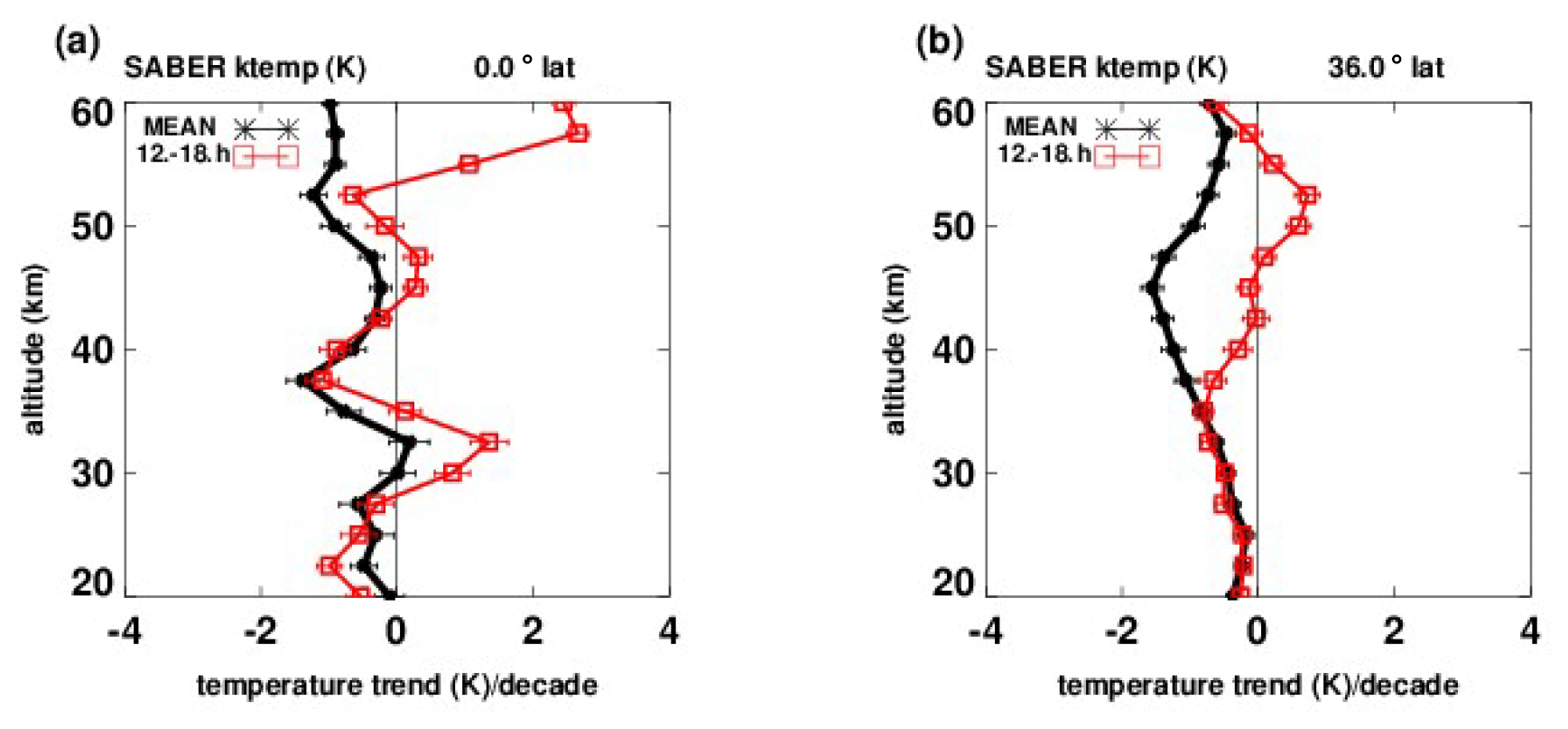
Figure 7Temperature trends (K per decade) vs. altitude at the Equator (a) and 36∘ N latitude (b). Black lines: trends based on SABER data (averaged over longitude and local time); red squares: estimated trends for cases where local times of measurements increase linearly from 12:00 to 18:00 LT from 2002 to 2014.
As noted earlier, over the years, the orbits of some operational satellites have drifted from their intended sun-synchronous state, so that the local times at which measurements are made have also drifted, by several hours. As a simple simulated example, Fig. 7 shows our results for temperature trends (K per decade) vs. altitude, at the Equator (Fig. 7a) and at 36∘ N, from 20 to 60 km. The red squares denote trends where local times increased linearly from 12:00 to 18:00 LT from 2002 to 2014, to simulate orbital drift. Black asterisks denote trends based on SABER data.
To the best of our knowledge, there have been no previous similar results on this subject, and Fig. 7 is meant to provide only an indication of what may result when the local times at which measurements are made are not controlled. Specifics depend on the orbital drift of the particular satellite (Funatsu et al., 2016) and on the particular study.
Using SABER data, we have investigated the local time variations of temperature trends (K per decade) for the years 2002 to 2014, from 20 to 100 km, for 48∘ S to 48∘ N latitude. SABER provides global temperature measurements over the 24 h of local time, and from 20 to 100 km in altitude, that are not available from other satellites and sources.
From our past studies based on SABER data, we estimated diurnal variations of the temperature (thermal tides) for each day, expressed in the form of five Fourier series components (Huang et al., 2010a).
We also derived zonal means of temperature that are averages over both longitude and local time for a circle of latitude (Huang et al., 2006, 2010a). These “synoptic” zonal means are important because they can then be compared directly with 3D models (Austin et al., 2008).
As explained earlier, zonal means from sun-synchronous satellites are tied to one or two local times. To the best of our knowledge, comparable zonal means of temperature that are averages over longitude and the 24 h of local time are not available elsewhere.
In this current study, we have combined past results to estimate the zonal mean trends corresponding to specific local times.
These results at local times have not been available previously. They show that the values of temperature decadal trends for a fixed local time are different from trends at another fixed local time. We find that the amplitudes and phases of the tides themselves also display decadal trends and are then likely contributors to the local time variations of temperature trends.
Our results of trend variations with local time are supported by comparisons with corresponding nighttime lidar measurements in the stratosphere and lower thermosphere. They are also supported by comparisons with corresponding satellite measurements made at specific local times in the stratosphere.
The dependence of trends on local time is significant throughout the region of analysis and can be significant even from hour to hour, as can be seen in Figs. 3–6.
The results for the lower thermosphere agree with corresponding trend results by She et al. (2019), based on lidar nighttime measurements. She et al. (2019) found that trends based on a 2 h average near midnight show systematic differences from the average over other hours. Our comparisons with the overnight results of She et al. (2019) are seen in Fig. 5, which shows that our trends at 19:00, 20:00, and 21:00 LT compare favorably, while our daytime trends at 15:00, 16:00, and 17:00 LT compare less favorably.
In the stratosphere, our comparison with trends found by Funatsu et al. (2016), based on lidar and AMSU measurements, is even better, as seen in Figs. 3 and 4. At 44∘ N (AMSU and OHP lidar), Funatsu et al. (2016) provide AMSU trend results only from 30 to 40 km, but they match our results almost exactly. Their results from 20 to 40 km, representing midlatitudes (30 to 60∘ N), also match our results almost exactly from 20 to 30 km but are larger from 30 to 40 km. Between ∼ 30 and 40 km, the nighttime lidar trends are significantly smaller (more negative) than both our trends and those of Funatsu et al. (2016). However, when the comparison is between nighttime lidar and our nighttime results (21:00, 22:00, and 23:00 LT; see Fig. 3a and b), the agreement is better. At 20∘ N (AMSU and MLO lidar), similar conclusions apply.
These examples all suggest that at least some of the differences between nighttime lidar trends and those based on other measurements that are not made at night can be explained, at least partly, through variations of trends with local time.
However, we emphasize that our three examples of course do not make a pattern, and more direct comparisons are needed. Our current comparisons are limited because the various results should be based on similar time spans and also not based on merged data from various sources, as the identity in local time would not be clear for merged data. Although there have been previous studies related to variations with local time, they focused on mitigating differences when merging data from different sources and on accounting for temperature variations with local time due to orbital drifts.
Because our results show that the data sets representing measurements at different fixed local times can result in varying trends, merging these data can result in trends that cannot be tied to specific local times or to averages over the 24 h of local time, as in 3D models, and can result in biases.
In this Appendix, we present additional figures, corresponding to Fig. 2b, of temperature diurnal amplitudes and phases over more altitudes (20, 40, 60, 80, 90 km) and latitudes (0, 40∘).
The left panels (a) of each figure show temperature tidal diurnal amplitudes and phases at various altitudes and the Equator, while the right panels (b) correspond to the left panels but at 40∘ N latitude. In each panel, the left axis scale and black line denote tidal diurnal amplitudes (K), while the right axis scale and red line show the diurnal phases (h of maximum value).
The displayed trend values are obtained from a simple least-squares straight line fit. The larger variations generally reflect modulation of the tides by the quasi-biennial oscillation (QBO). This has been discussed for models (Mayr and Mengel, 2005) and other SABER data (Forbes et al., 2008).
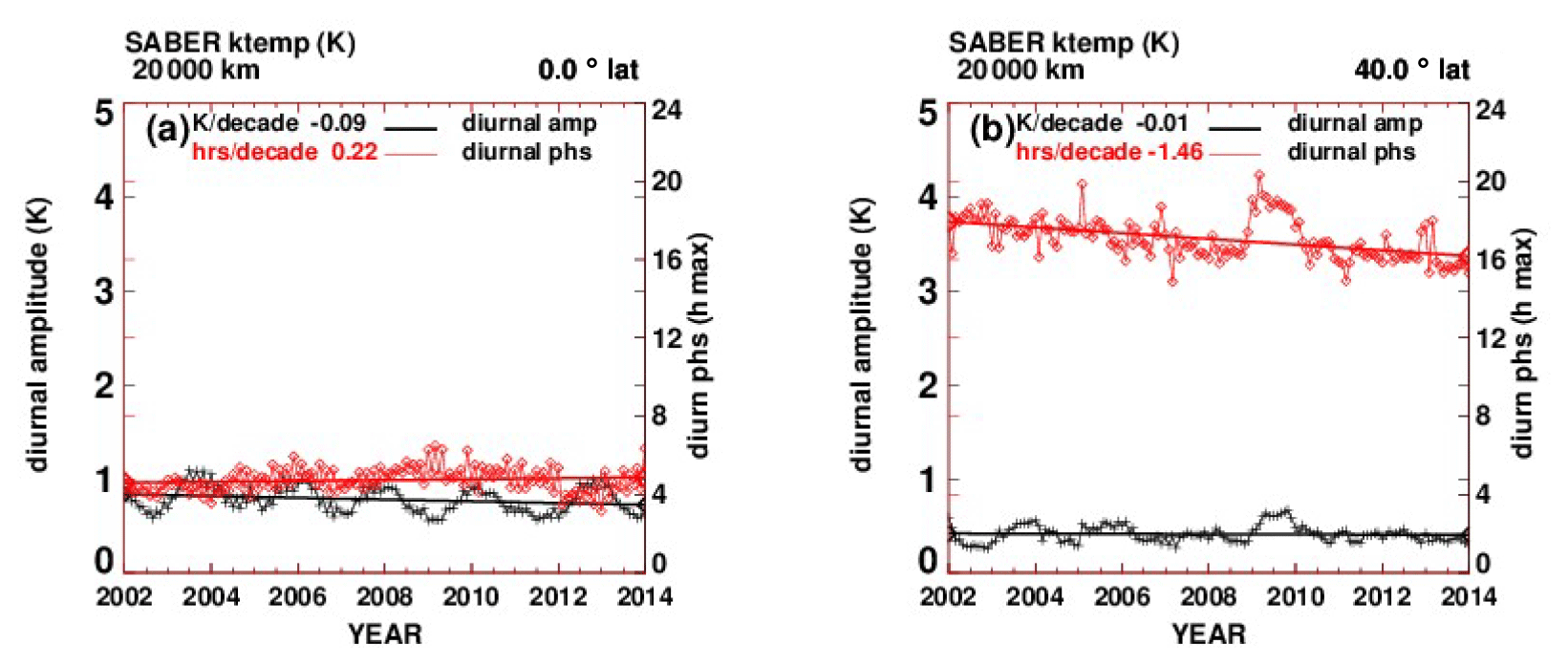
Figure A1(a) Temperature tidal diurnal amplitudes and phases at 20 km and the Equator. On the left axis scale, black line: tidal diurnal amplitude (K). On the right axis scale, red line: diurnal phase (h of maximum value). (b) As in (a) but at 40∘ N latitude.
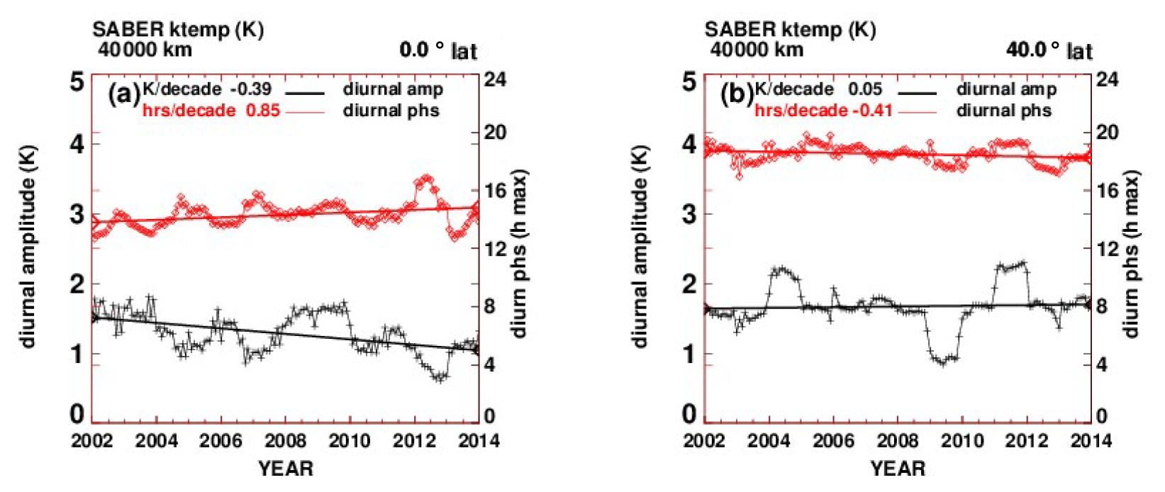
Figure A2(a) Temperature tidal diurnal amplitudes and phases at 40 km and the Equator. On the left axis scale, black line: tidal diurnal amplitude (K). On the right axis scale, red line: diurnal phase (h of maximum value). (b) As in (a) but at 40∘ N latitude.
Although the figures may give additional insight into the nature of the trends, there are caveats to be considered. We note that the semidiurnal amplitudes and phases can also be significant. We have derived a total of five Fourier components, and our numerical results reflect all five Fourier terms.
Because both amplitudes and phases exhibit trends, they need to be considered in parallel, in tandem, and this is difficult to discern qualitatively. In addition, because the trends are generally small, it is difficult to arrive at conclusions.
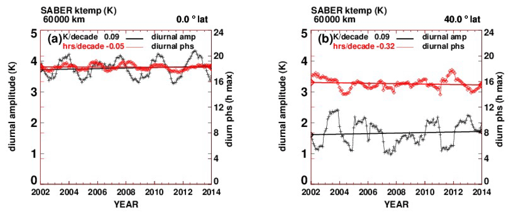
Figure A3(a) Temperature tidal diurnal amplitudes and phases at 60 km and the Equator. On the left axis scale, black line: tidal diurnal amplitude (K). On the right axis scale, red line: diurnal phase (h of maximum value). (b) As in (a) but at 40∘ N latitude.

Figure A4(a) Temperature tidal diurnal amplitudes and phases at 80 km and the Equator. On the left axis scale, black line: tidal diurnal amplitude (K). On the right axis scale, red line: diurnal phase (h of maximum value). (b) As in (a) but at 40∘ N latitude.

Figure A5(a) Temperature tidal diurnal amplitudes and phases at 90 km and the Equator. On the left axis scale, black line: tidal diurnal amplitude (K). On the right axis scale, red line: diurnal phase (h of maximum value). (b) As in (a) but at 40∘ N latitude.
The SABER data are freely available from the SABER project at http://saber.gats-inc.com/ (Russell and Mlynczak, 2015).
FH worked on the data analysis in addition to the science and interpretation of results. HG is a Principal Investigator on the TIMED/SABER satellite project and worked on the science and interpretation of the results, including effects of tides and their relation to the quasi-biennial oscillation (QBO).
The authors declare that they have no conflict of interest.
We thank the editor Gunter Stober and two anonymous referees, whose comments helped to improve the manuscript.
This paper was edited by Gunter Stober and reviewed by two anonymous referees.
Austin, J., Tourpali, K., Rozanov, E., Akiyoshi, H., Bekki, S., Bodeker, G., Brühl, C., Butchart, N., Chipperfield, M., Deushi, M., Fomichev, V. I., Giorgetta, M. A., Gray, L., Kodera, K., Lott, F., Manzini, E., Marsh, D., Matthes, K., Nagashima, T., Shibata, K., Stolarski, R. S., Struthers, H., and Tian, W.: Coupled chemistry climate model simulations of the solar cycle in ozone and temperature, J. Geophys. Res., 113, D11306, https://doi.org/10.1029/2007JD009391, 2008.
Brasseur, G. P. and Solomon, S.: Aeronomy of the Middle Atmosphere, Springer, Dordrecht, the Netherlands, 2005.
Forbes, J. M., Zhang, X., Palo, S., Russell, J, Mertens, C. J., and Mlynczak, M.: Tidal variability in the ionospheric dynamo region, J. Geophys. Res., 113, A02310, https://doi.org/10.1029/2007JA012737, 2008.
Funatsu, B. M., Claud, C., Keckhut, P., and Hauchecorne, A.: Cross-validation of Advanced Microwave Sounding Unit and lidar for long-term upper-stratospheric temperature monitoring, J. Geophys. Res., 113, D23108, https://doi.org/10.1029/2008JD010743, 2008.
Funatsu, B. M., Claud, C., Keckhut, P., Hauchecorne, A., and Leblanc, T.: Regional and seasonal stratospheric temperature trends in the last decade (2002–2014) from AMSU observations, J. Geophys. Res.-Atmos., 121, 8172–8185, https://doi.org/10.1002/2015JD024305, 2016.
Huang, F. T. and Mayr, H. G.: Ozone and temperature decadal solar-cycle responses, and their relation to diurnal variations in the stratosphere, mesosphere, and lower thermosphere, based on measurements from SABER on TIMED, Ann. Geophys., 37, 471–485, https://doi.org/10.5194/angeo-37-471-2019, 2019.
Huang, F. T., Mayr, H. G., Reber, C. A., Russell III, J. M., Mlynczak, M., and Mengel, J.: Zonal-mean temperature variations inferred from SABER measurements on TIMED compared withUARS observations, J. Geophys. Res., 111, A10S07, https://doi.org/10.1029/2005JA011427, 2006.
Huang, F. T., McPeters, R. D., Bhartia, P. K., Mayr, H. G., Frith, S. M., Russell III, J. M., and Mlynczak, M. G.: Temperature diurnal variations (migrating tides) in the stratosphere and lower mesosphere based on measurements from SABER on TIMED, J. Geophys. Res., 115, D16121, https://doi.org/10.1029/2009JD013698, 2010a.
Huang, F. T., Mayr, H. G., Russell III, J. M., and Mlynczak, M. G.: Ozone and temperature decadal trends in the stratosphere, mesosphere and lower thermosphere, based on measurements from SABER on TIMED, Ann. Geophys., 32, 935–949, https://doi.org/10.5194/angeo-32-935-2014, 2014.
Huang, F. T., Mayr, H. G., Russell III, J. M., and Mlynczak, M. G.: Ozone and temperature decadal responses to solar variability in the mesosphere and lower thermosphere, based on measurements from SABER on TIMED, Ann. Geophys., 34, 29–40, https://doi.org/10.5194/angeo-34-29-2016, 2016a.
Huang, F. T., Mayr, H. G., Russell III, J. M., and Mlynczak, M. G.: Ozone and temperature decadal responses to solar variability in the stratosphere and lower mesosphere, based on measurements from SABER on TIMED, Ann. Geophys., 34, 801–813, https://doi.org/10.5194/angeo-34-801-2016, 2016b.
Keckhut, P., Funatsu, B. M., Claud, C., and Hauchecorne, A.: Tidal effects on stratospheric temperature series derived from successive advanced microwave sounding units, Q. J. Roy. Meteor. Soc., 141, 477–483, https://doi.org/10.1002/qj.2368, 2015.
Khaykin, S. M., Funatsu, B. M., Hauchecorne, A., Godin-Beekmann, S., Claud, C., Keckhut, P., Pazmino, A., Gleisner, H., Nielson, J. K., Syndergaard, S., and Lauritsen, K. B.: Postmillennium changes in stratospheric temperature consistently resolved by GPS radio occultation and AMSU observations, Geophys. Res, Lett., 44, 7510–7518, https://doi.org/10.1002/2017GL074353, 2017.
Mayr, H. G. and Mengel, J. G.: Interannual variations of the diurnal tide in the mesosphere generated by the quasi-biennial oscillation, Geophys. Res, Lett., 110, D10111, https://doi.org/10.1029/2004JD005055, 2005.
McLandress, C., Shepherd, T. G., Jonsson, A. I., von Clarmann, T., and Funke, B.: A method for merging nadir-sounding climate records, with an application to the global-mean stratospheric temperature data sets from SSU and AMSU, Atmos. Chem. Phys., 15, 9271–9284, https://doi.org/10.5194/acp-15-9271-2015, 2015.
Mears, C. A. and Wentz, F. J.: Sensitivity of Satellite-Derived Tropospheric Temperature Trends to the Diurnal Cycle Adjustment, J. Climate, 29, 3629–3646, https://doi.org/10.1175/JCLI-D-15-0744.s1, 2016.
Mukhtarov, P., Pancheva, D., and Andonov, B.: Global structure and seasonal and interannual variability of the migrating diurnal tide seen in the SABER/TIMED temperatures between 20 and 120 km, J. Geophys. Res., 114, A02309, https://doi.org/10.1029/2008JA013759, 2009.
Nath, O. and Sridharan, S.: Long-termvariabilities and tendencies in zonal mean TIMED–SABER ozone and temperature in the middle atmosphere at 10–15∘ N, J. Atmos. Sol.-Terr. Phy., 120, 1–8, 2014.
Randel, W. J., Smith, A. K., Wu, F., Zou, C.-Z., and Qian, H.: Stratospheric temperature trends over 1979–2015 derived fromcombined SSU, MLS, and SABER satellite observations, J. Climate, 29, 4843–4859, https://doi.org/10.1175/JCLI-D-15-0629.1, 2016.
Russell III, J. M. and Mlynczak, M. G.: SABER data, available at: http://saber.gats-inc.com/, last access: 2015.
Russell III, J. M., Mlynczak, M. G., Gordley, L. L., Tansock, J., and Esplin, R.: An overview of the SABER experiment and preliminary calibration results, in: Proceedings of the SPIE, 44th Annual Meeting, Denver, Colorado, 18–23 July, 3756, 277–288, 1999.
She, C.-Y., Berger, U., Yan, Z.-A., Yuan, T., Lübken, F.-J., Krueger, D. A., and Hu, X.: Solar response and long‐term trend of midlatitude mesopause region temperature based on 28 years (1990–2017) of Na lidar observations, J. Geophys. Res.-Space, 124, 7140–7156, https://doi.org/10.1029/2019JA026759, 2019.
Zhang, X., Forbes, J. M., Hagan, M. E., Russell III, J. M., Palo, S. E., Mertens, C. J., and Mlynczak, M. G.: Monthly tidal temperatures 20–120 km from TIMED/SABER, J. Geophys. Res., 111, A10S08, https://doi.org/10.1029/2005JA011504, 2006.
Zou, C.-Z., Qian, H., Wang, W., Wang, L., and Long, C.: Recalibration and merging of SSU observations for stratospheric temperature trend studies, J. Geophys. Res., 119, 13180–13205, https://doi.org/10.1002/2014JD021603, 2014.