the Creative Commons Attribution 4.0 License.
the Creative Commons Attribution 4.0 License.
 | 16 Sep 2020
Magnetic field fluctuation properties of coronal mass ejection-driven sheath regions in the near-Earth solar wind
Emilia K. J. Kilpua
Dominique Fontaine
Simon W. Good
Matti Ala-Lahti
Adnane Osmane
Erika Palmerio
Emiliya Yordanova
Clement Moissard
Lina Z. Hadid
Miho Janvier
In this work, we investigate magnetic field fluctuations in three coronal mass ejection (CME)-driven sheath regions at 1 AU, with their speeds ranging from slow to fast. The data set we use consists primarily of high-resolution (0.092 s) magnetic field measurements from the Wind spacecraft. We analyse magnetic field fluctuation amplitudes, compressibility, and spectral properties of fluctuations. We also analyse intermittency using various approaches; we apply the partial variance of increments (PVIs) method, investigate probability distribution functions of fluctuations, including their skewness and kurtosis, and perform a structure function analysis. Our analysis is conducted separately for three different subregions within the sheath and one in the solar wind ahead of it, each 1 h in duration. We find that, for all cases, the transition from the solar wind ahead to the sheath generates new fluctuations, and the intermittency and compressibility increase, while the region closest to the ejecta leading edge resembled the solar wind ahead. The spectral indices exhibit large variability in different parts of the sheath but are typically steeper than Kolmogorov's in the inertial range. The structure function analysis produced generally the best fit with the extended p model, suggesting that turbulence is not fully developed in CME sheaths near Earth's orbit. Both Kraichnan–Iroshinikov and Kolmogorov's forms yielded high intermittency but different spectral slopes, thus questioning how well these models can describe turbulence in sheaths. At the smallest timescales investigated, the spectral indices indicate shallower than expected slopes in the dissipation range (between −2 and −2.5), suggesting that, in CME-driven sheaths at 1 AU, the energy cascade from larger to smaller scales could still be ongoing through the ion scale. Many turbulent properties of sheaths (e.g. spectral indices and compressibility) resemble those of the slow wind rather than the fast. They are also partly similar to properties reported in the terrestrial magnetosheath, in particular regarding their intermittency, compressibility, and absence of Kolmogorov's type turbulence. Our study also reveals that turbulent properties can vary considerably within the sheath. This was particularly the case for the fast sheath behind the strong and quasi-parallel shock, including a small, coherent structure embedded close to its midpoint. Our results support the view of the complex formation of the sheath and different physical mechanisms playing a role in generating fluctuations in them.
- Article
(4584 KB) - Full-text XML
-
Supplement
(494 KB) - BibTeX
- EndNote


Coronal mass ejection (CME)-driven sheath regions (e.g. Kilpua et al., 2017a) are turbulent large-scale heliospheric structures that are important drivers of disturbances in the near-Earth environment and present a useful natural laboratory for studying many fundamental plasma physical phenomena. Sheaths form gradually as the CME travels through the solar wind from the Sun to Earth, and they feature properties of both expansion and propagation sheaths (e.g. Siscoe and Odstrcil, 2008). As sheaths accumulate from layers of inhomogeneous plasma and magnetic field ahead, discontinuities and reconnection exhausts can be commonly found (e.g. Feng and Wang, 2013). Magnetic field fluctuations in the sheaths are both transmitted from the preceding solar wind and generated within the sheath, e.g. via physical processes at the shock and due to draping of the magnetic field around the driving ejecta (e.g. Gosling and McComas, 1987; Kataoka et al., 2005; Siscoe et al., 2007). Sheaths also embed various plasma waves; for instance, mirror mode and Alfvén ion cyclotron waves are frequently found (Ala-Lahti et al., 2018, 2019). The compressed and turbulent nature of the sheaths enhances solar wind–magnetosphere coupling efficiency when they interact with Earth's magnetic environment (Kilpua et al., 2017b). Sheaths have indeed been shown to be important drivers of geomagnetic storms (e.g. Tsurutani et al., 1988; Huttunen et al., 2002; Zhang et al., 2007; Echer et al., 2008; Yermolaev et al., 2010); in particular, they often cause intense responses in the high-latitude magnetosphere and ionosphere (e.g. Huttunen and Koskinen, 2004; Nikolaeva et al., 2011), they are related to intense and diverse wave activity in the inner magnetosphere (e.g. Kilpua et al., 2019b; Kalliokoski et al., 2020), and they produce drastic variations in high-energy electron fluxes in the Van Allen radiation belts (e.g. Hietala et al., 2014; Kilpua et al., 2015; Lugaz et al., 2015; Alves et al., 2016; Turner et al., 2019).
Despite their importance for heliophysics and solar–terrestrial studies, CME-driven sheath regions are currently investigated relatively little, and their multiscale structure is not well understood. In particular, a better understanding of the nature and properties of the magnetic field fluctuations in sheaths, and how these properties vary spatially within them, are crucial for understanding their formation and space weather impact. Detailed studies of magnetic field fluctuations in sheaths are also expected to yield new insight into outstanding problems in turbulence research, such as how intermittency in turbulence is related to the formation of coherent structures and discontinuities (e.g. current sheets) in plasmas.
Good et al. (2020) investigated the radial evolution of magnetic field fluctuations for a CME-driven sheath using almost radially aligned observations made by MESSENGER at ∼0.5 AU and STEREO B at ∼1 AU. At ∼0.5 AU, where the leading-edge shock was quasi-parallel, the downstream sheath plasma developed a range of large-angle field rotations, discontinuities, and complex structure that were absent in the upstream wind, with a corresponding steepening of the inertial-range spectral slope and an increase in the mean fluctuation compressibility in the sheath. At ∼1 AU, in contrast, the shock crossing was quasi-perpendicular and much less difference in fluctuation properties between the sheath plasma and upstream wind was observed. Intermittency in the sheath turbulence possibly grew between the spacecraft. The shock–sheath transition at MESSENGER had a qualitatively similar ageing effect on the plasma to that seen in the ambient solar wind with radial propagation between the two spacecraft. Moissard et al. (2019) performed a statistical investigation of magnetic field fluctuations in 42 CME-driven sheath regions observed in the near-Earth solar wind. In particular, the authors studied compressibility and anisotropy , where and P⟂ are the parallel and perpendicular power of fluctuations, respectively. They found that sheaths present increased compressibility and lower anisotropy when compared to the preceding solar wind or to the following CME ejecta. The total fluctuation power was also considerably (∼10 times) higher in the sheath than in the surrounding solar wind, consistent with some earlier studies (e.g. Kilpua et al., 2013). The fluctuation power was also found to be predominantly in the direction perpendicular to the magnetic field.
Properties of the driving CME and preceding solar wind are likely to have a significant role for turbulence in sheaths. Kilpua et al. (2013, 2019a) reported an increase in magnetic field fluctuation power with increasing CME speed. Moissard et al. (2019) found this same tendency and also emphasised the importance of the magnetic field fluctuation power in the preceding solar wind. A clear dependence of the inertial (magnetohydrodynamic) range spectra of the ion flux fluctuations on the large solar wind driver were found by Riazantseva et al. (2019), using high-resolution Spektr-R plasma data and Wind magnetic field data. They separated drivers into fast and slow solar wind, magnetic clouds and non-cloud ejecta, sheaths, and fast–slow stream interaction regions (SIRs; e.g. Richardson, 2018). They found, for example, that the inertial (magnetohydrodynamic) range spectral slopes in the slow solar wind, in sheaths ahead of non-cloud ejecta, and within magnetic clouds were less steep than the power law for Kolmogorov turbulence, while the slopes in the fast solar wind, in sheaths ahead of magnetic clouds, and within ejecta were closer to the Kolmogorov index. In the kinetic range, in turn, fluctuation spectra were steepest in compressive heliospheric structures, i.e. in sheaths and SIRs.
In this work, we analyse three CME-driven sheath regions in the near-Earth solar wind that present high, intermediate, and low speeds. The Mach numbers of the shocks preceding these sheaths range correspondingly from high (4.9) to low (1.8), and their shock angles range from quasi-parallel (33∘) to almost perpendicular (86∘). We investigate and compare distributions of the embedded magnetic field fluctuations, fluctuation amplitudes normalised to the mean magnetic field, compressibility, and intermittency. Our study is conducted for three separate 1 h periods within the sheaths, namely near the shock, in the middle of the sheath, and close to the ejecta leading edge. This division is applied because properties in sheath regions often change considerably from the shock to the ejecta leading edge, and magnetic field fluctuations in different parts can partly arise from different physical processes (e.g. Kilpua et al., 2019b). We also include in the study 1 h of the preceding solar wind for each event and investigate how fluctuation properties change from the solar wind to the sheath.
The manuscript is organised as follows: in Sect. 2 we describe the data sets used and some underlying assumptions. In Sect. 3 we present our analysis. First, we give a general overview of the three sheath events under study. Then, we investigate the properties of magnetic field fluctuations, spectral indices, and compressibility. Finally, we explore the intermittency of fluctuations in more detail by analysing distribution functions, skewness, kurtosis, and structure functions. In Sect. 4 we discuss, and in Sect. 5 we summarise our results.
We primarily use high-resolution magnetic field observations from the magnetic fields investigation (MFI; Lepping et al., 1995) instrument on board the Wind (Ogilvie and Desch, 1997) spacecraft. The magnetic field data during the observed events are available at 0.092 s cadence. We obtained the data through the NASA Goddard Space Flight Center Coordinated Data Analysis Web1 (CDAWeb). To provide an overview of the wider solar wind conditions for the studied events, we also used plasma data from Wind's solar wind experiment (SWE; Ogilvie et al., 1995) instrument, which are available at 90 s resolution. During the times of the events that are part of this study, Wind was located at the Lagrange L1 point.
In our analysis, we divide sheaths into three separate regions, each being 1 h in duration. Furthermore, we consider a 1 h region of solar wind preceding the shock and sheath, excluding the 30 min period immediately ahead of the shock. The three distinct regions within the sheath are termed the near-shock, mid-sheath, and near-leading edge (near-LE) regions. The near-shock region extends from the shock to the sheath, excluding the 15 min immediately following the shock, and the near-LE region ends 15 min before the leading edge of the interplanetary coronal mass ejections (ICMEs) ejecta. The 15 min interval closest to the shock and the ejecta leading edge have been excluded to avoid the shock transitions and most immediate shock processes and uncertainties in the timing of the ejecta leading edge, respectively. The mid-sheath regions are located around the middle of the sheath, except for the fast event for which the mid-sheath region was selected to capture a coherent magnetic field structure embedded in the sheath. We, however, emphasise that the results for the mid-sheath are likely to depend strongly on the selected interval.
The fluctuations in the magnetic field are defined here as , and fluctuation amplitude , where Δt is the timescale or time lag between two samples. We use 14 values of Δt that range from 0.092 to 736 s (12.3 min), where the values are successively doubled. The observations thus cover most of the inertial range (101 s ≲Δt≲103 s) and the upper part of the sub-ion (kinetic) range (Δt≲101 s).
We study magnetic field fluctuations in the spacecraft frame, which is in relative motion with respect to the solar wind frame. To justify the transformation from spacecraft frequency to wavenumber, and to relate observed timescales to length scales in the plasma, the so-called Taylor hypothesis (Taylor, 1938; Matthaeus and Goldstein, 1982) must be valid. The hypothesis states in this context that when the timescales of the magnetic field fluctuations are much less than the timescale of rapidly flowing solar wind, the path of a spacecraft travelling through solar wind represents an instantaneous spatial cut. This can be expressed in a simple way as (Howes et al., 2014), where vA is the Alfvén speed, and v the solar wind speed. The results are shown in Table 1, where it can be seen that for all events and subregions the criterion is met in this study.
3.1 Event overview
We analyse three CME-driven sheath regions detected by the Wind spacecraft in the near-Earth solar wind at the Lagrange L1 point. The key parameters of these events are listed in Table 1. The events were selected from the list of 81 sheaths published in Kilpua et al. (2019b) to have their speeds represent the lowest, median, and highest speeds of the whole population. The speed of the sheath was selected as our primary parameter for the event selection since solar wind turbulence studies often consider slow and fast wind separately due to their different evolution and origin, which affects their turbulent properties. We also required that the selected sheaths were at least 4 h in duration, were followed by a well-defined CME ejecta that was classified as a magnetic cloud in the Richardson and Cane ICME list2 (Richardson and Cane, 2010), presented a clear transition from the sheath to the ejecta, and that no other CMEs were present within a 1 d period prior to the interplanetary shock ahead of the sheath. The selected events are as follows: 14–15 December 2006 (fast sheath), 24–25 October 2011 (medium-speed sheath), and 31 October 2012 (slow sheath), with their mean speeds calculated over the duration of the whole sheath being 880, 503, and 351 km s−1, respectively. Table 1 also shows that the investigated events also have different shock strengths and shock speeds. The fast sheath was preceded by the strongest and fastest shock (4.9 and 919 km s−1), while the slow event was preceded by the weakest and slowest shock (1.8 and 391 km s−1). The shock angles (θBn; i.e., the angle between the shock normal and upstream magnetic field) also varied amongst the events; while the fastest sheath was associated with a quasi-parallel shock (33∘), the intermediate and slow sheaths were preceded by quasi-perpendicular shocks. For the slowest sheath, the shock angle was very close to the perpendicular (θBn=86∘). The shock configuration is also expected to affect magnetic field fluctuation properties in the sheath, in particular in the near-shock region (e.g. Bale et al., 2005a; Burgess et al., 2005).
Table 1Summary of the events analysed. The first two rows give the shock and CME ejecta leading edge (LE) times at Wind. The following rows give the shock parameters, namely magnetosonic Mach number (Mms), shock angle (θBn; i.e. the angle between the shock normal and upstream magnetic field), shock speed (Vshock), and upstream plasma beta (βu). The next rows give the sheath parameters, namely the duration of the sheath (ΔT), the average solar wind speed in the sheath (〈Vsheath〉), the average magnetic field magnitude (〈Bsheath〉), the parameter κ, defined as and tests the validity of the Taylor hypothesis (see Sect. 2 for details), and the planar magnetic structure (PMS) coverage, which indicates the percentage of the sheath subregions occupied by PMS-type field behaviour (see Sect. 3.1). The last rows give the average solar wind speed and κ values for the 1 h solar wind interval preceding the shock.
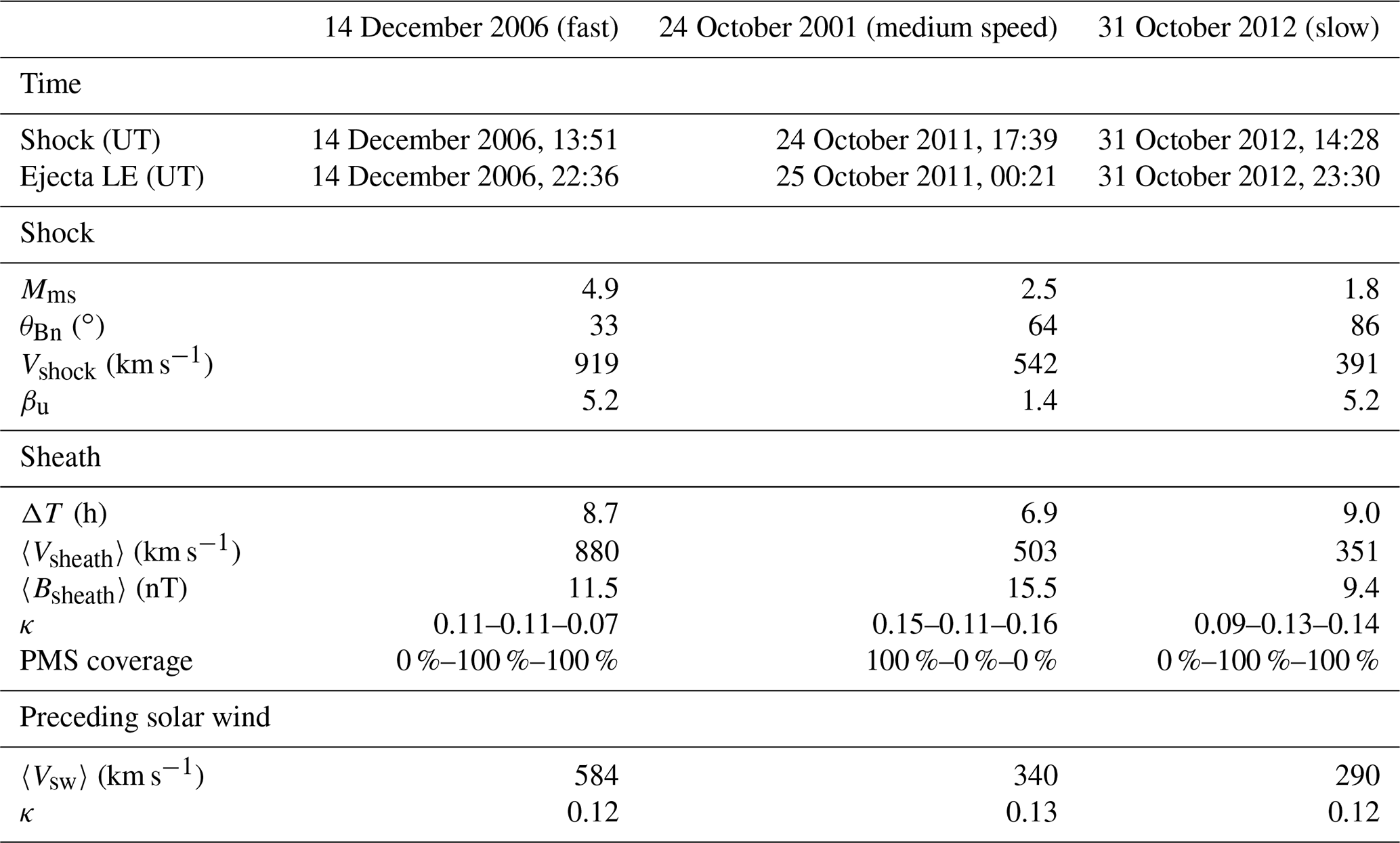
Figure 1 shows the solar wind conditions during the three events under study. The orange shaded intervals show the 1 h regions subject to a more detailed analysis. The first four panels give the interplanetary magnetic field (IMF) magnitude, IMF components in geocentric solar ecliptic (GSE) coordinates (blue – BX; green – BY; and red – BZ), solar wind speed, and density. It is clear that all three cases present well-defined sheath regions, with large-amplitude magnetic field fluctuations embedded, and enhanced solar wind density. It is, however, evident that the overall properties of the sheath vary considerably between the three events and from the shock to ejecta leading edge. We also note that the fast sheath is preceded by fast solar wind, while the medium-speed and slow sheaths are preceded by slow wind. The largest fluctuations seem to be associated with the north–south magnetic field component (BZ).
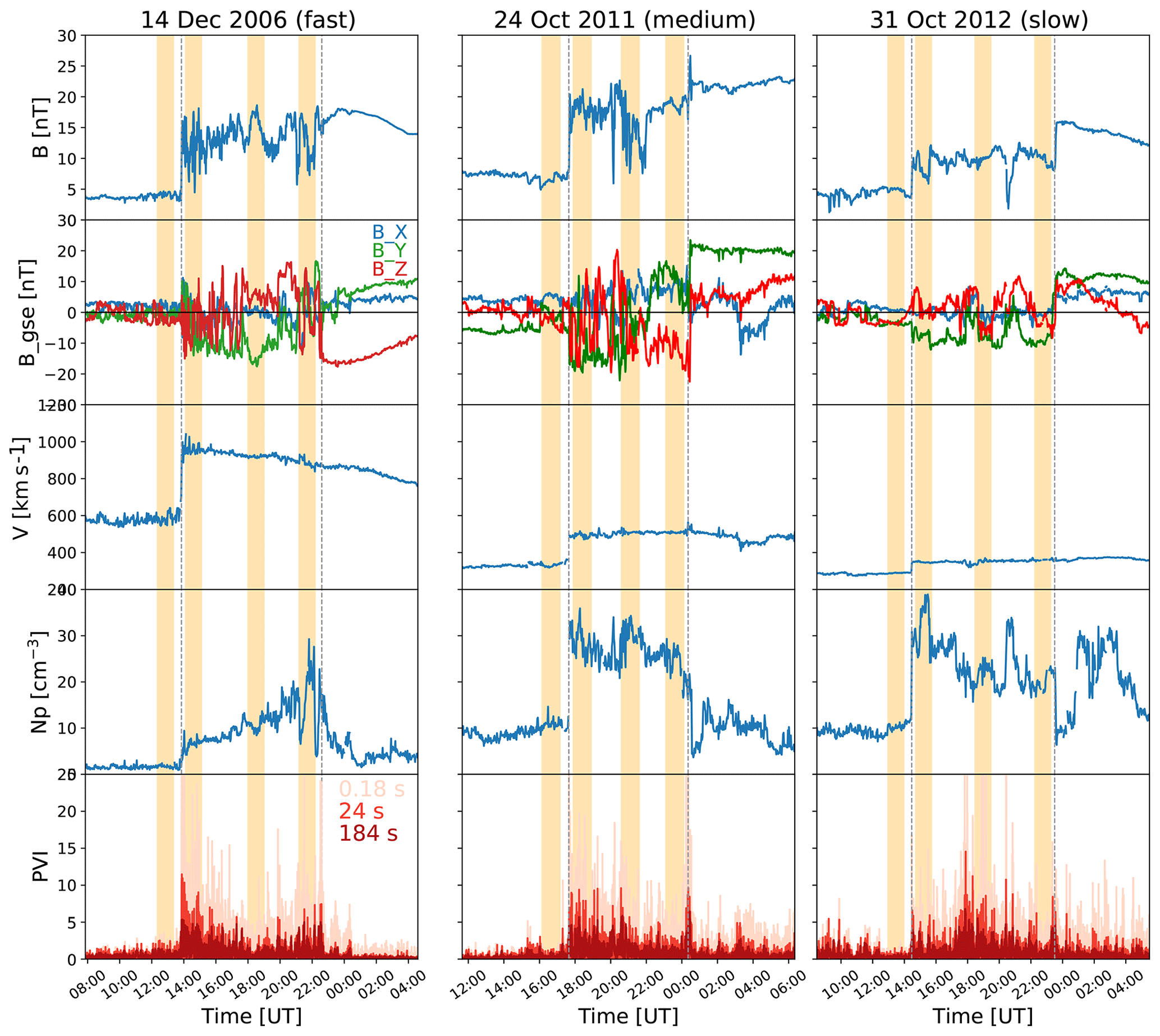
Figure 1Interplanetary magnetic field and plasma parameters measured at Wind near the Lagrange L1 point for the three analysed events. The panels give the (a) magnetic field magnitude, (b) magnetic field components in GSE coordinates (blue – BX; green – BY; and red – BZ), (c) solar wind speed, (d) density, and (e) partial variance of increments (PVIs) values calculated for 0.18, 24, and 184 s. The orange shaded regions show the 1 h region in the preceding solar wind and those representing three different parts of the sheath, namely near-shock, mid-sheath, and near-LE regions.
The last panel of Fig. 1 gives the normalised partial variance of increments (PVIs). The PVI parameter is defined as follows:
where the average in the denominator is taken over the whole interval shown. This quantity is used to detect coherent structures or discontinuities (e.g. Greco et al., 2018; Zhou et al., 2019). We calculate the PVI here using three different time lags between two data points, namely Δt=0.18, 24, and 186 s (with 0.18 s corresponding to the kinetic range, and 24 and 186 s corresponding to the inertial range). The figure shows that the PVI exhibits a number of spikes throughout most of the sheaths investigated, suggesting that intermittent structures are frequently present. The largest PVI spikes in the fast and medium-speed sheath occur close to the shock, while for the slow sheath they are found close to the middle part of the sheath. The coherent structure in the fast sheath exhibits a low PVI. Another interesting feature visible from the PVI panel is that the near-LE regions, in particular for the medium-speed and slow sheaths, have similar PVI levels to the solar wind ahead of them (excluding the peaks at the sheath–ejecta transition).
Table 1 shows the percentage of the sheath subregions occupied by planar magnetic structures (PMSs) determined with the method described in Palmerio et al. (2016). PMSs are periods during which the variations of the magnetic field vectors remain nearly parallel to a fixed plane over an extended time period (e.g. Nakagawa et al., 1989; Jones and Balogh, 2000). PMSs typically cover a significant part of the sheath and can be present in all parts of the sheath (Palmerio et al., 2016). In CME-driven sheaths, they are thought to arise from processes at the shock (i.e. the alignment and amplification of pre-existing discontinuities; e.g. Neugebauer et al., 1993; Kataoka et al., 2005) and field line draping around the CME ejecta (e.g. Gosling and McComas, 1987). As reported by Kataoka et al. (2005) and Palmerio et al. (2016), PMSs are most frequently found behind strong quasi-perpendicular shocks with high upstream plasma beta. The fast sheath and the slow one had no PMSs in their near-shock region, but their mid-sheath and near-LE regions were fully covered by planar fields. The lack of PMSs in the near-shock region for the fast sheath is likely due to the quasi-parallel shock configuration, while for the slow sheath it is probably due to its leading shock being weak (Mms=1.8). The medium-speed sheath, in turn, presented planar fields in the near-shock region but no PMSs in the other subregions. The comparison of planar periods with the PVI values shown in Fig. 1 does not reveal an obvious correlation.
3.2 Distributions and averages of magnetic field fluctuations
Figure 2 shows the probability distribution functions (PDFs) of the normalised fluctuation amplitude δB∕B for timescales Δt ranging from 0.092 s (light red) to 736 s (dark red). δB is defined in Sect. 2, and B is the mean magnetic field amplitude calculated over the time interval Δt. This approach is similar to, for example, Chen et al. (2015), Matteini et al. (2018), and Good et al. (2020). These studies have indicated that, in the solar wind, fluctuations have predominantly small normalised fluctuation amplitudes (δB∕B values <1) at smaller Δt, but PDFs spread to larger δB∕B values at larger Δt. δB∕B values exceeding signify large directional changes in the field (exceeding 90∘), while values >2 indicate that fluctuations must be at least partly compressional (e.g. Chen et al., 2015). Note that for purely Alfvénic (i.e. incompressible) fluctuations the field magnitude does not change, and δB∕B must be <2. The columns show, from left to right, different subregions and, from top to bottom, the three different events.

Figure 2Probability distribution functions of δB∕B for different timescales Δt (shown as curves in different colours) for (top) 14 December 2006, (middle) 24 October 2011, and (bottom) 31 October 2012 events. The leftmost columns give the results for the solar wind preceding the shock, and the following three columns represent the three different sheath subregions.
The solar wind preceding the medium-speed and slow sheaths has practically all δB∕B values <1 (left panels of Fig. 2), meaning that there are no significant rotations of the field direction (no larger than 60∘ for the pure rotation case). The fast event (14 December 2006), in turn, is preceded by a solar wind with clearly larger normalised fluctuation amplitudes. The δB∕B values are nevertheless mostly <2, suggesting that fluctuations are largely Alfvénic (see above). We also note that the solar wind ahead of the fast sheath could be affected by foreshock waves since it is ahead of the quasi-parallel shock, as discussed in Sect. 3.1.
Comparison of the preceding solar wind and near-shock regions shows that the normalised fluctuation amplitudes are spread to considerably larger values in the near-shock region for all events and timescales investigated. This can be due to the generation of new fluctuations or amplification (in magnitude and/or change in the field direction) of pre-existing fluctuations relative to the mean field. For the medium-speed and slow sheath distributions, δB∕B values are mostly confined to in the near-shock region, which means that there are no significant rotations, while for the fast sheath there is a significant fraction of values >2 for scales Δt≳6 s, meaning that large rotations of the field direction exist and fluctuations must be at least partly compressional.
Figure 2 clearly shows that the PDFs vary considerably in different sheath subregions. This is particularly evident in the fast sheath. Both the near-shock and near-LE regions have PDFs extending to , but for the near-LE region this occurs for the larger timescales only (Δt≳48 s), i.e. at scales within the inertial range, while for the near-shock regions PDFs populate for Δt≳1.5 s. Within the small coherent structure near the middle of the fast sheath, fluctuations are, in turn, restricted to , thus being much smaller than in the other parts of the sheath or preceding solar wind. For the medium- and slow-speed sheaths, the largest δB∕B values occur in the mid-sheath region, and in the case of the medium-speed sheath, δB∕B exceeds 2 for the largest scales.
One interesting feature in Fig. 2 is that the near-LE distributions resemble those in the solar wind ahead quite closely, both in terms of their extent of higher δB∕B values and shape of the curves. This is most distinct for the medium-speed and slow sheaths for which δB∕B values are mostly confined to <1. For the fast sheath, distributions in the near-LE region at larger scales are, however, clearly flatter and less smooth than in the solar wind ahead (or in the near-shock region).
Figure 2 also reveals the expected general trend; for the smallest timescales, PDFs have sharp peaks at low δB∕B values and then decay exponentially, while at larger timescales the distributions become broader, in particular in the sheaths. This behaviour, i.e. that distributions of normalised fluctuations become more Gaussian and shift towards larger values with increasing timescales, is consistent with previous studies carried out in the solar wind (e.g. Sorriso-Valvo et al., 2001; Chen et al., 2015; Matteini et al., 2018). We will return to investigate this in more detail in Sect. 3.5.1.
We now consider the average fluctuation amplitudes across the range of timescales. The top and middle panels of Fig. 3 show the mean values of δB and δB∕B as a function of timescale. In the top panel, the ion cyclotron timescales (tci) are also plotted, using the mean magnetic field magnitude over the whole subregion in question. tci is obtained as an inverse of ion cyclotron frequency (fci) doppler shifted to the spacecraft frame, using ; see e.g. Chen et al. (2015).
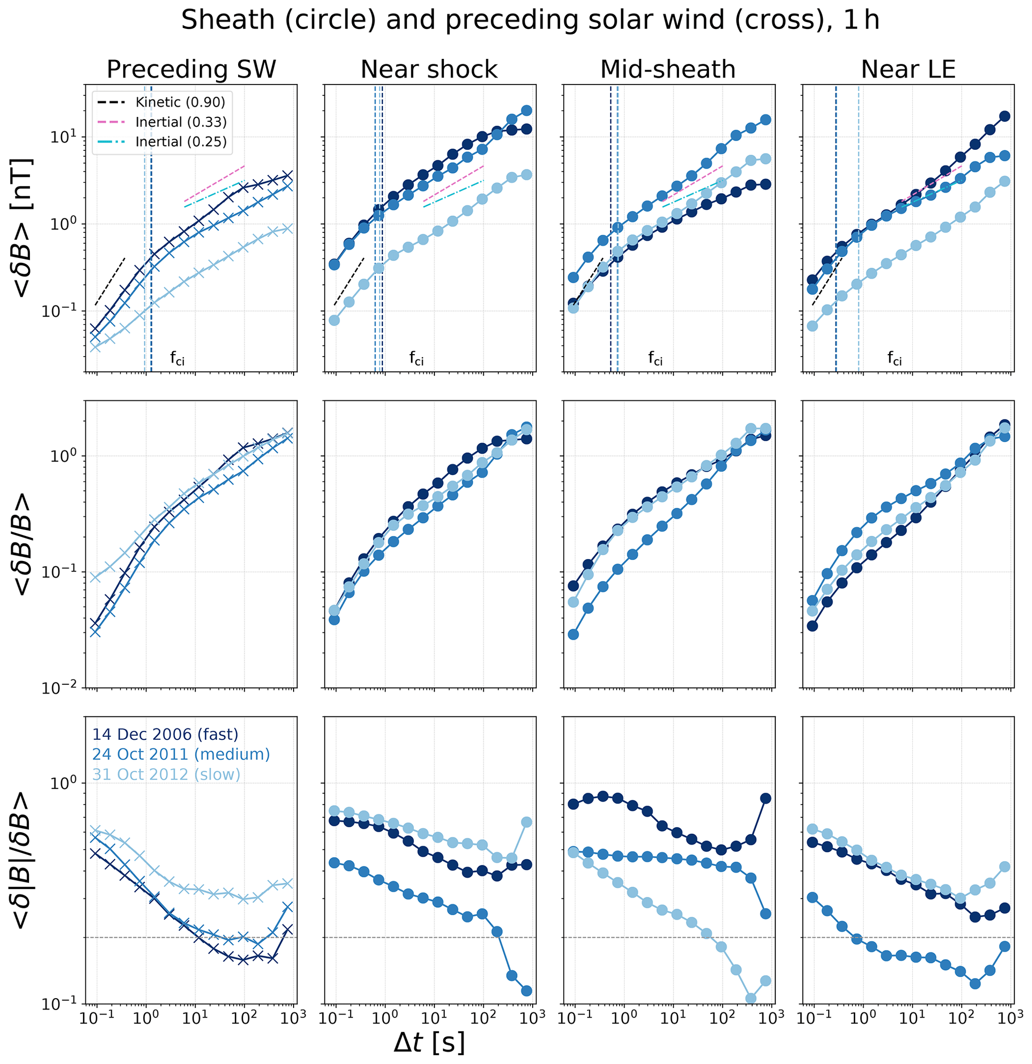
Figure 3Means of fluctuation amplitudes 〈δB〉, normalised fluctuations 〈δB∕B〉, and fluctuation compressibility as functions of timescale Δt. Results are shown separately for the preceding solar wind (crosses) and three different regions of the sheaths (circles). Different colours represent fast (dark blue), intermediate speed (medium blue), and slow (light blue) sheaths. The dashed vertical lines show the ion cyclotron scales calculated using the magnetic field magnitude averaged over the region in question.
In the preceding solar wind intervals, mean fluctuation amplitudes 〈δB〉 and normalised fluctuation amplitudes 〈δB∕B〉 are highest ahead of the fast sheath and lowest ahead of the slow sheath. We, however, note that differences are relatively small, in particular for the mean fluctuation amplitudes between the fast and medium-speed sheath. As is to be expected when considering the field compression at the shock, 〈δB〉 are considerably higher in the near-shock region than in the preceding solar wind for all events and timescales. The 〈δB∕B〉 values are also higher in the near-shock and mid-sheath regions than in the solar wind ahead, which is also reported in Good et al. (2020). This suggests that the transition from the solar wind to the sheath generates new and/or enhances pre-existing magnetic field fluctuations at all timescales.
Matteini et al. (2018) reported that the spectra of normalised fluctuation amplitudes collapsed on the same curve for the solar wind periods observed by Helios and Ulysses, suggesting the modulation of the field fluctuations with the magnetic field magnitude. Their results were, however, obtained at varying heliospheric distances and solar wind speeds. In our study, 〈δB〉 curves are organised according to the solar wind speed as mentioned above. This trend is maintained throughout the sheath, except for the small coherent structure in the midpoint of the fast sheath that exhibits both lower 〈δB〉 and 〈δB∕B〉 values (especially so at larger scales) than in the solar wind ahead or in the mid-sheath regions of the other two sheaths.
3.3 Spectral indices
Several studies have investigated how the power spectrum of solar wind magnetic field fluctuations is in agreement with predictions made by turbulence theories (e.g. Coleman, 1968; Bavassano et al., 1982; Horbury and Balogh, 2001; Bale et al., 2005b; Tsurutani et al., 2018; Verscharen et al., 2019). Kolmogorov's spatially homogeneous hydrodynamic turbulence model gives (i.e. spectral index ; Kolmogorov, 1941) and is based on the assumption that energy cascades from larger to smaller scales through eddies that break down evenly and are space filling. The modification of Kolmogorov's model for a magnetohydromagnetic fluid, based on works by Iroshnikov (1964) and Kraichnan (1965), takes into consideration the interactions between oppositely propagating Alfvén waves and equipartitioning between magnetic and kinetic energy. In the inertial regime of the Kraichnan–Iroshinikov model, the energy spectrum is proportional to (i.e. spectral index ), i.e. less steep than in the Kolmogorov model. The energy is then dissipated in the kinetic range, and the breakpoint occurs around the ion cyclotron scale (, where fci is the ion cyclotron frequency). The kinetic regime exhibits a steeper spectral slope than the inertial regime, with spectral index typically reported in the solar wind (e.g. Alexandrova et al., 2013; Bruno et al., 2017; Huang et al., 2017). The timescales studied here should generally be below the energy-driving f−1 regime, which occurs at frequencies f≳10−3 Hz for the fast wind, i.e. timescales ≳16.7 min (e.g. Bruno and Carbone, 2013), and at frequencies f≳10−4 Hz, i.e. timescales ≳166.7 min or 2.7 h for the slow wind (e.g. Bruno, 2019). This regime, known as the energy-containing scale, is likely composed of fluctuations with various origins and remains debated (see e.g. discussion in Bruno et al., 2019). We note that some of the curves in the top panels of Fig. 3, in particular the preceding solar wind and near-shock subregions in the fast sheath, exhibit a flattening trend towards the largest timescales that could indicate the transition to the f−1 regime. Another possibility is that, as discussed in Sect. 3.2, foreshock waves can affect, and could result in, a small hump seen at timescales around 100 s.
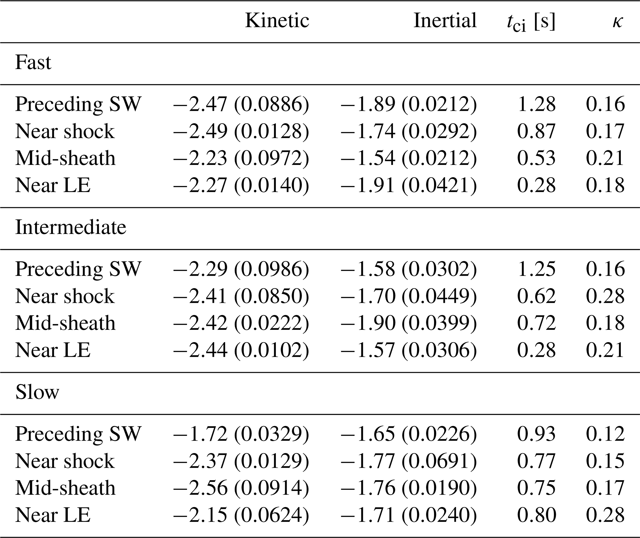
The 〈δB∕B〉 values in the top panels of Fig. 3 can be used to calculate the slopes, as their gradients are related to turbulence in the inertial range. This stems from the connection of δB2 at scale l to k-space spectral power P(k) as , where and P(k)≈kα (e.g. Matteini et al., 2018; Good et al., 2020). The pink dashed lines l0.33 in Fig. 3 show the Kolmogorov scaling, and the cyan dashed and dotted lines l0.25 show the Kraichnan–Iroshinikov scaling in the inertial range. Note that the l0.33 and l0.25 given in the figure correspond to and , respectively (e.g. Matteini et al., 2018). In the kinetic range we have plotted the scaling l0.9 (). Table 2 shows the kinetic and inertial range spectral indices for the preceding solar wind and in the three subregions of the sheath. The kinetic range indices are determined using the first three timescales from 0.092 to 0.37 s, and the inertial range indices are determined using five timescales from 6 to 96 s. The timescales used to calculate the inertial scale indices are above the ion cyclotron timescales for all cases and fall into the region where the 〈δB〉 curves have approximately a linear behaviour (see Fig. 3). They are also well above the 0.3 Hz (3 s) of the dissipation range breakpoint found in the extensive statistical study at the Lagrange L1 point by Smith et al. (2006).
In the kinetic range, the spectral slopes are consistently less steep than the −2.8 index cited above. For the solar wind preceding the slow sheath, the kinetic range spectral index is −1.72, while in other regions they are distributed between −2.23 and −2.49. In the inertial range the spectral indices vary considerably. The near-shock region for the fast sheath, near-shock, and near-LE regions for the medium-speed sheath and the preceding solar wind region for the slow sheath have their inertial range spectral indices matching or close to the Kolmogorov index (−1.67). The mid-sheath region for the fast sheath and the preceding solar wind for the medium-speed sheath exhibit, in turn, their spectral index close to the Kraichnan–Iroshinikov value (−1.5). Otherwise, the spectral indices are clearly steeper than Kolmogorov's. For the fast sheath, the slope in the preceding solar wind region could have been affected by the possible foreshock-wave-related hump (see above), and the slope could be, in reality, closer to Kolmogorov's.
Table 2Spectral indices as calculated by fitting a straight line in log space for kinetic range (Δt=0.092–0.37 s; three consecutive time lags) and inertial range (Δt=24–96 s; five consecutive time lags). The values in the parenthesis show the standard deviation errors associated with the fitting. The third column gives the ion cyclotron period for each region. The last column gives that tests the validity of the Taylor hypothesis (see Sect. 2 for details).
3.4 Compressibility
The bottom panels of Fig. 3 show the mean of . This parameter gives the compressibility of magnetic fluctuations, i.e. the mean amount of compression as a fraction of the total fluctuation amplitude, as a function of timescale. The horizontal line is at (Matteini et al., 2018), which represents the typical upper threshold of the level of compressibility in magnetic field fluctuations found for the fast solar wind in the inertial regime; the slow solar wind tends to have values exceeding 0.2.
For all cases investigated, compressibility increases from the solar wind ahead to the near-shock region, suggesting that the locally generated new fluctuations in the sheath are at least partly compressible. This occurs for all timescales for the fast and slow sheaths. For the medium-speed sheath the two largest scales show a decrease, with compressibility values <0.2. Again, it is possible that this decrease at the largest scales is due to a larger statistical error since the magnetic field magnitude does not change that much in this subregion when compared to other events. The solar wind preceding the fast sheath has values below 0.2 in the inertial range, consistent with its speed being in the fast wind range (see Fig. 1).
Figure 3 shows that the level of compressibility varies considerably in different subregions of the sheath. For the fast sheath, compressibility is relatively high in all sheath subregions and above the preceding solar wind values, in particular in the small coherent structure near the middle of the sheath. This is in agreement with normalised fluctuation amplitudes 〈δ∕B〉 being low in the region (Sect. 3.2), as compressible and/or parallel fluctuations are known to have lower amplitudes and/or power than Alfvénic and/or perpendicular fluctuations (i.e. there is power anisotropy). For the medium-speed sheath, compressibility values are also high in the mid-sheath, but in the near-LE region, in turn, fluctuations are even less compressible than in the preceding solar wind and for most timescales below 0.2. The slow sheath has most compressible fluctuations in the near-shock and near-LE regions, comparable to values for the fast sheath, but in the mid-sheath region compressibility values fall below the preceding solar wind values and even the 0.2 threshold for the largest timescales (Δt>96 s). In all instances, it can be seen that compressibility generally decreases from the smallest scales until about 100 s. This is a well-known trend from previous solar wind studies (e.g. Chen et al., 2015; Matteini et al., 2018; Good et al., 2020). We note that the increase for the few highest timescales could be related to statistical errors in the data, as discussed above.
3.5 Intermittency
Several studies have shown that fluctuations in the solar wind are typically strongly intermittent (e.g. Burlaga, 1991; Feynman and Ruzmaikin, 1994; Marsch and Tu, 1994, 1997; Pagel and Balogh, 2001; Yordanova et al., 2009). Intermittency describes the inhomogeneity in the energy transfer between scales and is manifested as a lack of self-similarity in fluctuation distributions between scales (see, e.g., reviews by Horbury et al., 2005; Sorriso-Valvo et al., 2005; Bruno, 2019; Verscharen et al., 2019). In the solar wind, it can arise from coherent structures, such as current sheets and discontinuities. The PVI parameter shown in the bottom panel of Fig. 1 already gives some indication that intermittent structures were embedded throughout the sheaths analysed.
3.5.1 Probability distribution functions
Deviations from a Gaussian distribution in fluctuation PDFs at different timescales can reveal the presence of intermittency. Figure 4 shows distributions of for different Δt values. Here, σ is the standard deviation and μ the mean of δBZ calculated using a 15 min sliding average. The black dashed line shows the normal distribution for which the standard deviation and mean correspond to that of the distribution calculated using the 6 s timescale, but we note that normal distributions for the other timescales shown would be almost inseparable from the 6 s curve. Similar PDFs for BX and BY are shown in the Supplement (Figs. S1 and S2). We investigate here in detail the Z component of the IMF since it has the largest importance for the solar wind magnetosphere coupling and geo-efficiency of the sheath. We note that PDFs for different components are overall very similar, but BZ has somewhat heavier tails than the other components (also suggesting higher intermittency). This is consistent with Fig. 1, which shows the largest amplitude fluctuations for BZ.
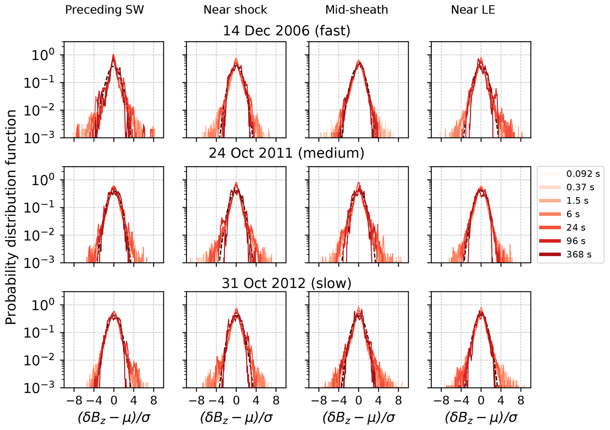
Figure 4Probability distribution functions of (where μ is the average and σ is the standard deviation of δBZ calculated over a 15 min sliding window) for different timescales Δt (shown as curves in different colours) for (top) 14 December 2006, (middle) 24 October 2011, and (bottom) 31 October 2012 events. The leftmost columns give the results for the solar wind preceding the shock, and the following three columns give the results for three different sheath subregions. The black dashed line shows the Gaussian for 6 s timescale.
The distributions in Fig. 4 are clearly non-Gaussian and particularly so at smaller timescales (light red curves) where they are spikier and have flatter tails; these are clear signs of intermittency. At larger timescales (dark red curves), distributions become generally more Gaussian, consistent with, e.g., Greco et al. (2008). Non-self-similarity is also qualitatively evident in Fig. 4.
3.5.2 Skewness and kurtosis
In order to characterise the non-Gaussian aspects of the distributions, we compute the higher-order moments. Figure 5 gives the skewness and kurtosis calculated for the distributions shown in Fig. 4. Skewness is related to the third distribution moment and gives information on the degree of distribution asymmetry. For the normal distribution, skewness is zero, i.e. the distribution is symmetric around the mean value. Positive skewness indicates an extended tail at larger values than the mean (i.e. weighting and a longer tail towards the right), whereas negative skewness indicates an extended tail at smaller values than the mean (i.e. weighting and a longer tail towards the left). Kurtosis is related to the fourth distribution moment and can be used as the proxy of large fluctuations that are an indication of intermittency (e.g. Krommes, 2002; Osmane et al., 2015). PDFs with long tails have larger kurtosis than narrow PDFs. For the normal distribution, kurtosis is 3; values larger than 3 indicate flatter tails, while values less than 3 indicate lighter tails. In Fig. 5 we have subtracted the value 3 from the kurtosis, so that 0 depicts the normal distribution for both kurtosis and skewness.
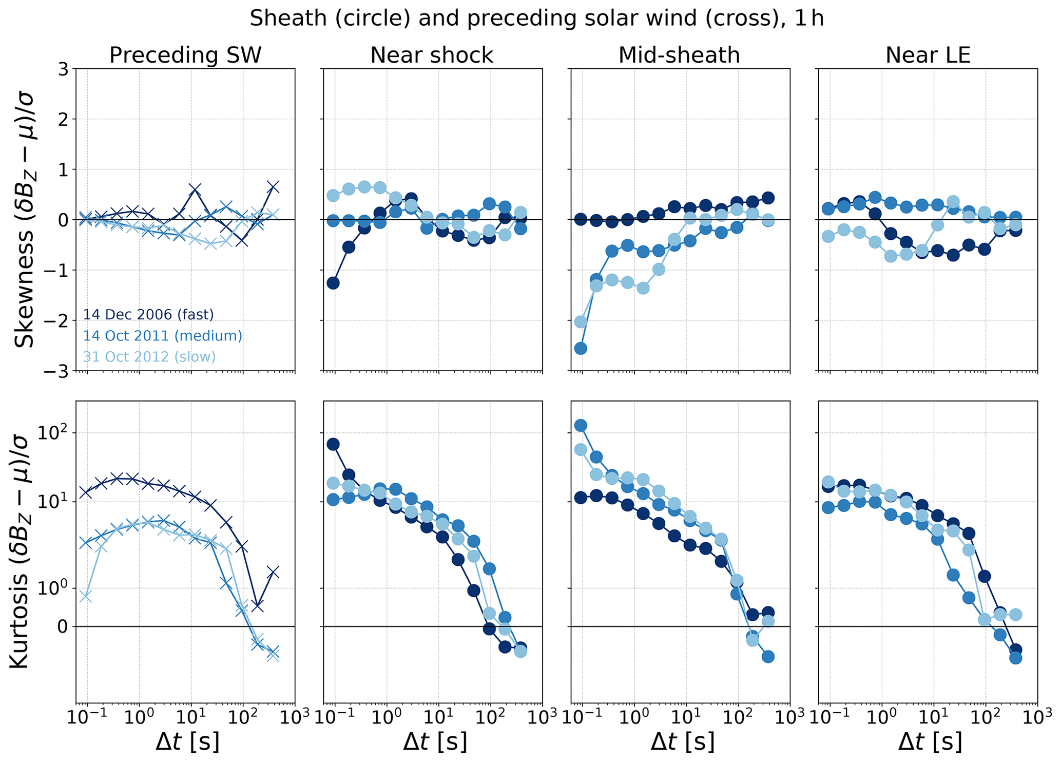
Figure 5Skewness (top) and kurtosis (bottom) calculated for δBZ as a function of timescale Δt. Different colours and panels represent the fast (dark blue), intermediate speed (medium blue), and slow (light blue) sheaths. The dots indicate the values in the sheath, and the crosses indicate the values in the preceding solar wind.
For all investigated subregions skewness has mostly small absolute values (<1), suggesting that distributions and fluctuations are generally symmetric around the mean (∼0 nT). There are no obvious drastic differences in skewness between the preceding solar wind and the sheath. One feature visible from the plot is that, for all events, the skewness in the preceding sheath tends to have stronger negative values, signifying that there is an excess of negative fluctuations, while in the solar wind ahead both negative and positive skewness values are observed more evenly. The largest absolute magnitudes of skewness (i.e. indicating largest asymmetries when compared to a Gaussian distribution) are found for the medium-speed and slow sheaths in the mid-sheath region.
The kurtosis values are nearly all positive, indicating an excess of high-amplitude δBZ fluctuations with respect to the normal distribution. In the majority of cases, kurtosis decreases towards zero through the inertial range, indicating that distributions become more Gaussian with increasing timescales. This is consistent with the qualitative assessment of distribution shapes discussed in Sect. 3.5.1. In the solar wind, kurtosis peaks broadly near the small-scale end of the inertial range and reduces in value with decreasing scale through the kinetic range (most clear for the medium-speed and slow event). Across the same scales in the sheaths, in contrast, kurtosis flattens or continues to increase with reducing scale. Peaks in kurtosis are associated with the inertial–kinetic spectral breakpoint (e.g. Chen et al., 2015); the ion cyclotron period (Table 1), which is in the vicinity of this spectral break, is larger in the preceding solar wind than in the sheaths, which may partly explain the more obvious kurtosis peaks. There is also a clear general increase in kurtosis between the solar wind ahead and near-LE regions for the slow and intermediate-speed events, while there is no significant change in values for the fast event. This could indicate that the near-LE distributions are less peaked for the fast sheath, i.e. in contrast to the behaviour of the medium-speed and slow sheaths.
3.5.3 Structure function analysis
Intermittency can be also investigated using structure functions (e.g. Bruno and Carbone, 2013). The structure function of order m of the fluctuation amplitude in the ith magnetic field component is as follows:
If the system conforms to a self-similar scaling law, then . The scaling exponent is (i.e. ) in Kolmogorov's turbulence and in the Kraichnan–Iroshinikov model.
To account for intermittency and inhomogeneities in the energy transfer between scales, various turbulence models have been proposed in the literature (see a more detailed description from, e.g., Horbury and Balogh, 1997; Bruno, 2019). Several models have been shown to fit observations reasonably well; for brevity, only results for the p model are shown here. We note that other models were tested, e.g. the random β model (Frisch et al., 1978; Paladin and Vulpiani, 1987) and the She–Lévêque model (She and Leveque, 1994), but it was found that the p model agreed best with the observed structure function scaling.
The standard p model by Meneveau and Sreenivasan (1987, see also Tu et al., 1996) assumes fully developed turbulence in which intermittency arises from the unequal breakdown of eddies, i.e. resulting daughter eddies having different amounts of energy. The structure function scaling exponents in the p model are defined as follows:
where the intermittency parameter p varies between 0.5 and 1. The parameter q is 3 in the Kolmogorov form and 4 for the Kraichnan–Iroshinikov form (e.g. Carbone, 1993). The p value of 0.5 corresponds to the non-intermittent case, giving for Kolmogorov and for Kraichnan–Iroshinikov turbulence. In the non-intermittent case, the structure function scaling exponents are linear with the moment m. Where there is intermittency, the scaling exponents flatten for larger m and curves become nonlinear. The maximum intermittency in both cases occurs for p=1, i.e. g(m)=1.
The extended p model (Tu et al., 1996; Marsch and Tu, 1997) describes turbulence that is not fully developed, as has been identified, for example, in the inner heliosphere. In the Kolmogorov form, it is as follows:
and in the Kraichnan–Iroshinikov form, as follows:
Here two parameters, namely p and α′, are needed to describe the turbulence cascade because the cascade depends on the scale for underdeveloped turbulence. Thus, the power spectral index is not linearly related to the second-order structure function exponent (as is the case for fully developed turbulence) but includes spatial inhomogeneity. The intermittency parameter, p, again gives the spatial inhomogeneity of the cascade rate, while the α′ parameter is the intrinsic spectral slope describing the scaling properties of the space-averaged cascade rate. The first terms on the right-hand sides of the previous two equations now represent the scale dependence of the cascade, and the second terms represent intermittency. The spectral index is related to the intrinsic spectral index and p parameter in the Kolmogorov form, as follows:
and in the Kraichnan–Iroshinikov form, as follows:
Structure functions up to m=4 only have been calculated since our 1 h data intervals (with sampling resolution of 0.092 s) include only approximately 39 130 data points (see, e.g., discussion in Horbury and Balogh, 1997). The scaling indices are calculated over timescales from 6 to 96 s within the inertial range (see Sect. 3.3). The results are given for the total structure function obtained by summing together the structure functions of the three components of the magnetic field as, for example, in Pei et al. (2016).
In Fig. 6, the standard p model scaling exponent curves are plotted as a function of m for p=0.5–1. The observational results are shown as lime-green crosses (solar wind ahead) and dots (sheath subregions). Orange curves correspond to Kolmogorov (K) scalings and blue curves correspond to Kraichnan–Iroshinikov (K–I) scalings for varying amounts of intermittency, p. The grey horizontal line gives the maximum intermittency case (i.e. p=1; g(m)=1), and the pink and cyan curves give the non-intermittent (i.e. p=0.5) cases corresponding to Kolmogorov and Kraichnan–Iroshinikov turbulence, respectively. The thick black curves show the best nonlinear least square fits to the extended p model.
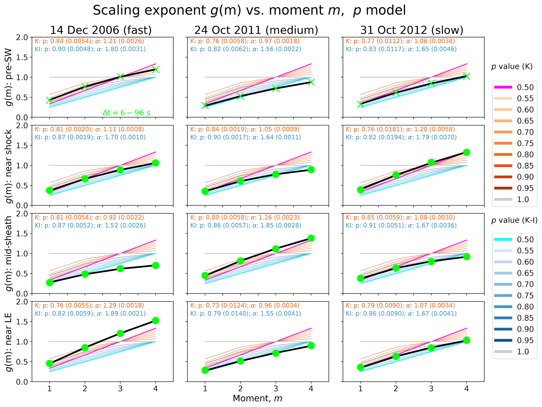
Figure 6The dots and crosses show the scaling exponent g(m) for the structure function as a function of moment m (m is set to range from 1 to 4) for the preceding solar wind and three subregions of the sheath. The orange and blue curves show the results for the standard p model, with p ranging from 0.5 to 1 in steps of 0.05 for the Kolmogorov's (K) and Kraichnan–Iroshinikov (K–I) forms, respectively. The non-intermittent cases (p=0.5) are shown in pink (K) and cyan (K–I), while the grey horizontal curve gives the maximum intermittency case (p=1). The bright green dots show the results calculated for timescales Δt=6–96 s, corresponding to the inertial range. The thick black line shows the least square fits for the extended p model. The values show the values of p and α parameters for the Kolmogorov's (orange) and Kraichnan–Iroshinikov (blue) forms, with standard deviation errors in parenthesis.
We note that, for the majority of cases, the standard p model curves do not match well with the observed g(m) curve (lime-green dots and crosses); there are either significant deviations between the observed and modelled points, the observed points do not follow the model trends, or both. The best agreement with the standard p model is with the solar wind ahead of the fast sheath, consistent with the Kolmogorov form at high p values (∼0.85). The near-shock region of the fast sheath and the solar wind ahead the slow sheath coincide, in turn, relatively closely with the Kraichnan–Iroshinikov form of the standard p model, also at high p values. In all other cases, the observed values deviate from the standard p model curves, particularly deeper in the fast sheath.
In both intermittent and non-intermittent cases, the structure function should have either g(3)=1 for the Kolmogorov scaling or g(4)=1 for the Kraichnan–Iroshinikov scaling. There are several regions in our data events for which neither g(3)≈1 nor g(4)≈1 hold. We note that significant deviations from these values can give rise to false non-intermittent signatures as discussed, e.g., in Pagel and Balogh (2002).
The extended p model can be fitted with the data with excellent agreement, and the Kolmogorov and Kraichnan–Iroshinikov forms overlap (black thick curve). However, these two forms of the model yield very different p and α values; these values are given in the panels of Fig. 6, with the corresponding standard deviation errors in parenthesis. The errors are of the order 10−3. We note that the Kraichnan–Iroshinikov form fits yield consistently larger p values than the Kolmogorov form fits but both indicate high intermittency. The values of spectral indices given by the Kraichnan–Iroshinikov form are, however, clearly more consistent with the spectral indices shown in Table 2 that were calculated for the fitting for 〈δB〉 using the same timescale range.
We have investigated magnetic field fluctuations in three CME-driven sheath regions observed in the solar wind at the Lagrange L1 point. Three parts of the sheath were studied separately, corresponding to the regions just adjacent to the shock (near shock), at or near the middle of the sheath (mid-sheath), and adjacent to the ejecta leading edge (near LE). The results were also compared with the solar wind preceding the sheaths.
For all three cases, we found that the spectral and turbulent properties differed considerably between the preceding solar wind and the sheath. This was the case despite very different overall event properties, e.g. the speed of the sheath and preceding shock, shock angle and strength, level of upstream fluctuations, and upstream solar wind speed and plasma beta. This is in contrast with the sheath analysed by Good et al. (2020), who found clear differences between the solar wind ahead and in the sheath at the orbit of Mercury but not near the orbit of Earth. However, they investigated fluctuations throughout the sheath collectively, while we have investigated three subregions separately. The sheath analysed in their work was slow and, at Earth's orbit, the preceding shock had a quasi-perpendicular configuration. In our study, we emphasise that some clear changes between the solar wind ahead and sheaths occurred (particularly in the near-shock subregion), including the slow sheath preceded by an almost-perpendicular shock.
First, distributions of normalised magnetic field fluctuations were flatter and spread to considerably higher values in the near-shock region than in the preceding solar wind for all events. For the fast sheath in particular, values demonstrated the existence of significant rotations and compressional fluctuations. This is expected as the processes at the shock are more efficient the faster and stronger the shock is; for example, fast shocks are expected to cause alignment and amplification of pre-existing solar wind discontinuities more efficiently, provide more free energy for wave generation, etc. (e.g. Neugebauer et al., 1993; Kataoka et al., 2005; Kilpua et al., 2013; Ala-Lahti et al., 2018, 2019). The quasi-parallel nature of the shock could also have enhanced the fluctuations for the fast event. For all cases, the distribution of the magnetic field fluctuations in the near-LE region appear quite similar to those in the pre-existing solar wind (consistent with the PVI results). The kurtosis analysis revealed further details as more peaked near-LE distributions for medium and slow sheaths. We also note that, in the inertial range, spectral indices were the most similar between the solar wind ahead and the near-LE region. This could be understood by considering that the part of the sheath closest to the ejecta leading edge is not affected by the shock, and, for the slower sheaths, processes at the leading edge are not affected that much either. The near-LE region of the fast sheath had, however, distinctly flat δB∕B distributions and extended tails when compared to the solar wind ahead and the slower sheaths. This could indicate an effective magnetic field draping process by the CME ejecta. As discussed by Gosling and McComas (1987) and McComas et al. (1988), the amount of draping increases with the CME speed. The detailed connection of the draping to sheath small-scale structures has, however, not yet been established. The mean amplitudes and normalised amplitudes of fluctuations were higher in the sheath than in the preceding solar wind, which is expected as the shock compresses the plasma and field ahead.
The compressibility was also generally higher in the sheath than in the preceding solar wind, suggesting that the new fluctuations that were generated in the transition from the solar wind ahead to the ejecta were mostly compressible. We also found that, in terms of compressibility, sheaths behave more like the slow solar wind than the fast wind; i.e., we found values above 0.2 to dominate in the sheath, which is in agreement with what is found for the slow wind (Bavassano et al., 1982; Bruno and Carbone, 2013). This was also the case for the fastest sheath in our study that was preceded by fast wind, with values below 0.2.
The inertial range spectral indices in our study for sheath subregions were mostly clearly steeper than Kolmogorov's spectral index of −1.67. Borovsky (2012) reported steeper slopes for the magnetic field fluctuations for the slow solar wind (spectral index −1.7) than for the fast wind (spectral index −1.54). This also suggests that turbulence in sheaths more resembles turbulence in the slow wind than in the fast wind. We, however, emphasise that spectral indices in our study exhibited quite large variability. Interestingly also, the fast solar wind ahead of the fast sheath had a steeper spectral index than the slow solar wind ahead of the medium-speed and slow sheaths, which had their spectral indices close to Kraichnan–Iroshinikov's and Kolmogorov's values, respectively. This could be, however, related to the interference of foreshock waves. The kinetic range spectral indices in turn indicated consistently shallower slopes (spectral indices varying from about −2.1 to −2.5) than what is on average observed in the solar wind (spectral index ; see Sect. 3.3). Several previous studies have also reported that, in the solar wind, both kinetic and inertial spectral indices exhibit a large range of values (e.g. Leamon et al., 1998; Smith et al., 2006; Borovsky, 2012). This is the case also in the magnetosheath (e.g. Alexandrova et al., 2008). The inertial range spectral indices in the solar wind tend to also steepen towards Kolmogorov's with increasing distance from the Sun (e.g. Bavassano et al., 1982). Sahraoui et al. (2009) reported average spectral indices matching our values (from −2.3 to −2.5) in their study of magnetic field fluctuations in the near-Earth solar wind using Cluster observations for about a 3 h time interval in the frequency range 4–35 Hz (i.e. 2.5–0.03 s). They observed another spectral breakpoint at 35 Hz, close to the electron gyro-scale, after which the slopes further steepened with the spectral index (see also Sahraoui et al., 2010; Alexandrova et al., 2013; Bruno et al., 2017). Sahraoui et al. (2009) argued that only a relatively small part of the energy is damped at ion scales where the kinetic Alfvén wave cascade still occurs from larger to smaller scales, whereas most of the dissipation occurs in the electron scales where the observed slopes were much steeper. The observations we used in our study are not high cadence enough to capture this second breakpoint, but the kinetic range spectral indices being close to those of Sahraoui et al. (2009) imply that this could also generally be the case for CME-driven sheath regions. The statistical study of Huang et al. (2017) found that, in the Earth's magnetosheath in the inertial scale, the spectral indices were close to −1, resembling thus the energy-driven scale in the solar wind rather than Kolmogorov's . Spectral indices close to Kolmogorov's were only observed further away from the bow shock at the flanks and close to the magnetopause. The majority of the events were dominated by compressible magnetosonic-like fluctuations.
We investigated intermittency using various methods. First, we found that the PVI values are generally high in the sheaths when compared to the ambient solar wind, suggesting that sheaths frequently embed intermittent structures. This is in agreement with Zhou et al. (2019). Our analysis of the kurtosis and distributions of normalised fluctuations also suggests that sheaths have, in general, high intermittency. Generally, intermittency increases with distance from the Sun and is higher in the fast, rather than in the slow, wind (Pagel and Balogh, 2001; Wawrzaszek et al., 2015; Bruno, 2019). The slow wind in turn shows strong variability in its intermittency (e.g. Pagel and Balogh, 2002). The fact that CME-driven sheaths feature high intermittency at 1 AU suggests that intermittent structures are actively formed during the formation and evolution of sheaths in interplanetary space. This is consistent with sheaths being heliospheric structures that gather over long periods of time (up to several days near the Earth's orbit), from inhomogeneous solar wind plasma that is compressed and processed at the CME shock and then piles up at the ejecta leading edge. Good et al. (2020) also found a possible increase in intermittency for their slow CME sheath from Mercury's orbit to Earth's orbit. The authors suggested that it likely is due to the development of intermittent structures, for example, current sheets in the sheath during CME propagation. This scenario is consistent with generally steep inertial range spectral indices in CME-driven sheaths as current. As suggested by, for example, the analysis in Li et al. (2012), current sheets in the solar wind could generally steepen the spectra. We also note that our analysis hinted that intermittency in BZ is larger than in BX or BY. This is an interesting point for future research and could be related to processes in action at the shock and/or CME leading edge creating, in particular, out-of-ecliptic magnetic field fluctuations (e.g. field line draping discussed in the Introduction).
Our structure function analysis showed that the standard p model did not generally match the observed g(m) curve features. The best match was found for the fast solar wind preceding the fast sheath. The extended p model, however, yielded a very good fit both for the Kolmogorov and Kraichnan–Iroshinikov forms, and the curves were indistinguishable. This has been the case also in some previous studies in the solar wind (e.g. Horbury and Balogh, 1997; Horbury et al., 1997) and has also been reported for the studies of turbulence in Earth's magnetosheath (e.g. Yordanova et al., 2008) and in the magnetospheric cusp (e.g. Yordanova et al., 2004). In addition, the Kraichnan–Iroshinikov form yielded consistently larger intermittency parameter p and α values, also reported earlier (e.g. Tu et al., 1996; Yordanova et al., 2004). They also clearly matched better with the indices we obtained from the fitting of the mean magnetic field fluctuations for the corresponding timescales. These findings would suggest that turbulence in the sheath is not fully developed at the orbit of Earth and is more consistent with the Kraichnan–Iroshinikov picture than Kolmogorov's; i.e., sheaths would behave more like a magnetofluid, which would agree with sheaths being structures with high magnetic field magnitudes. We note that previous studies have also reported that the Kraichnan–Iroshinikov form produces better fits, particularly in cases of solar wind periods with a strong magnetic field (e.g. Podesta, 2011). The results are, however, partly contradictory in the sense that the slopes were Kraichnan–Iroshinikov-like (−1.5) only for a few cases. It could be that CME-driven sheaths can embed plenty of structures (current sheets with large amplitude and large angle directional field changes, magnetic holes, reconnection exhausts, plasma interfaces, and plasma blobs) even in relatively short periods of time and are thus not described so well by the current turbulent models. Li et al. (2012) also suggested that Kolmogorov-like spectra in the solar wind could also result from the presence of intermittent current sheets where the field direction changes rapidly; i.e., as a consequence, the spectra would steepen from Kraichnan–Iroshinikov to Kolmogorov.
Our study highlights that turbulent properties can vary strongly within the sheath and are controlled by various factors, including the properties of the solar wind ahead; for example, its plasma beta and level of turbulence, the shock strength and configuration, path of the spacecraft through the shock–sheath–ejecta structure, and the properties of the driving CME ejecta, in particular by its speed (Kilpua et al., 2013; Moissard et al., 2019). The variations were in general most drastic for the fastest sheath and most subtle for the slowest sheath in our study. We emphasise that we investigated only one subregion in the middle of the sheath here, and it would be interesting to study how turbulent properties vary across the whole sheath from the shock to the ejecta leading edge, e.g. by applying a sliding window. Our study also revealed a small-scale coherent structure within the 14 December 2006 fast sheath. This substructure had distinct properties featuring, for example, clearly depressed δB∕B values, high compressibility, and a very shallow spectral slope with an inertial range spectral index close to Kraichnan–Iroshinikov's value. Regarding intermittency, compressibility, and general absence of Kolmogorov's type turbulence, CME sheaths (in particular in regions close to the shock) are similar to planetary magnetosheaths, which implies the universality of those properties in a compressible medium and also the universality regarding the role of the shock in destroying the correlation between the turbulent fluctuations in the solar wind, as discussed in Huang et al. (2017). The f−1 spectrum was, however, not found.
To summarise, based on our case study of three CME-driven sheath regions observed at the Lagrange L1 point, the magnetic field fluctuation amplitudes, normalised fluctuation amplitudes, and compressibility are enhanced in the sheath when compared to the solar wind ahead. The transition to the sheath thus generates new fluctuations and/or amplifies (in magnitude and/or change in the field direction) pre-existing fluctuations relative to the mean field. The intermittency was also found to be higher in the sheath than in the preceding solar wind for many of the investigated subregions. These findings applied for all three sheaths involved, featuring different speeds, shock strengths, and shock angles. Turbulent properties and spectral indices also varied quite considerably between the studied events and the sheath subregions, which reflects the complex structure and formation process of the sheaths of various properties. In general, turbulence in sheaths resembles that of the slow solar wind, and we found this to be valid even for the fast sheath preceded by fast wind. According to our study, turbulence in the sheath is not fully developed, likely due to processes that are constantly in action at the shock and close to the ejecta leading edge as the CME ploughs its way through interplanetary space. This can also explain the high intermittency in sheaths. We also found indications that, in sheaths, the energy cascade from larger to smaller scales could still be partly ongoing at the ion scales, which suggests that the majority of the dissipation would occur at electron scales (not captured by our study).
Future studies focusing more deeply on how sheath turbulence varies from the shock to the ejecta leading edge and extensive statistical studies connecting sheath properties to preceding solar wind and driver characteristics would shed light on these issues. The Parker Solar Probe (Fox et al., 2016) and the Solar Orbiter (Müller et al., 2013) will also make it possible to analyse sheath properties and turbulence with varying heliospheric distances and possibly provide multi-spacecraft encounters of CME sheaths, allowing us to probe how sheath characteristics evolve from the nose of the shock to the CME flanks.
The Wind data were obtained through CDAWeb (https://cdaweb.sci.gsfc.nasa.gov/index.html/; NASA, 2020).
The supplement related to this article is available online at: https://doi.org/10.5194/angeo-38-999-2020-supplement.
EKJK did the main data analysis and compiled the figures. EKJK, DF, and SWG planned the majority of the research and approaches to be used in the study. EP performed the PMS analysis. All authors contributed to the methods and physical interpretations and to the writing of the paper.
The authors declare that they have no conflict of interest.
The results presented herein have been achieved under the framework of the Finnish Centre of Excellence in Research of Sustainable Space (Academy of Finland; grant no. 1312390), which we gratefully acknowledge. This project has received funding from the European Research Council (ERC) under the European Union's Horizon 2020 research and innovation programme (grant no. ERC-COG 724391). Emilia K. J. Kilpua acknowledges the Academy of Finland project, SMASH (grant no. 310445). Erika Palmerio's research was supported by the NASA Living With a Star Jack Eddy Postdoctoral Fellowship program, administered by UCAR's Cooperative Programs for the Advancement of Earth System Science (CPAESS; grant no. NNX16AK22G). Emiliya Yordanova's research was supported by the Swedish Civil Contingencies Agency (MSB; grant no. Dnr.2016-2102).
This research has been supported by the European Research Council (SolMAG; grant no. 724391), the Academy of Finland, Luonnontieteiden ja Tekniikan Tutkimuksen Toimikunta (grant no. 1312390), the Academy of Finland, Luonnontieteiden ja Tekniikan Tutkimuksen Toimikunta (grant no. 310445), the NASA Living With a Star Jack Eddy Postdoctoral Fellowship Program (grant no. NNX16AK22G), and the Swedish Civil Contingencies Agency (grant no. 2016-2102).
This paper was edited by Anna Milillo and reviewed by two anonymous referees.
Ala-Lahti, M., Kilpua, E. K. J., Souček, J., Pulkkinen, T. I., and Dimmock, A. P.: Alfvén Ion Cyclotron Waves in Sheath Regions Driven by Interplanetary Coronal Mass Ejections, J. Geophys. Res.-Space, 124, 3893–3909, https://doi.org/10.1029/2019JA026579, 2019. a, b
Ala-Lahti, M. M., Kilpua, E. K. J., Dimmock, A. P., Osmane, A., Pulkkinen, T., and Souček, J.: Statistical analysis of mirror mode waves in sheath regions driven by interplanetary coronal mass ejection, Ann. Geophys., 36, 793–808, https://doi.org/10.5194/angeo-36-793-2018, 2018. a, b
Alexandrova, O., Lacombe, C., and Mangeney, A.: Spectra and anisotropy of magnetic fluctuations in the Earth's magnetosheath: Cluster observations, Ann. Geophys., 26, 3585–3596, https://doi.org/10.5194/angeo-26-3585-2008, 2008. a
Alexandrova, O., Chen, C. H. K., Sorriso-Valvo, L., Horbury, T. S., and Bale, S. D.: Solar Wind Turbulence and the Role of Ion Instabilities, Space Sci. Rev., 178, 101–139, https://doi.org/10.1007/s11214-013-0004-8, 2013. a, b
Alves, L. R., Da Silva, L. A., Souza, V. M., Sibeck, D. G., Jauer, P. R., Vieira, L. E. A., Walsh, B. M., Silveira, M. V. D., Marchezi, J. P., Rockenbach, M., Lago, A. D., Mendes, O., Tsurutani, B. T., Koga, D., Kanekal, S. G., Baker, D. N., Wygant, J. R., and Kletzing, C. A.: Outer radiation belt dropout dynamics following the arrival of two interplanetary coronal mass ejections, Geophys. Res. Lett., 43, 978–987, https://doi.org/10.1002/2015GL067066, 2016. a
Bale, S. D., Balikhin, M. A., Horbury, T. S., Krasnoselskikh, V. V., Kucharek, H., Möbius, E., Walker, S. N., Balogh, A., Burgess, D., Lembège, B., Lucek, E. A., Scholer, M., Schwartz, S. J., and Thomsen, M. F.: Quasi-perpendicular Shock Structure and Processes, Space Sci. Rev., 118, 161–203, https://doi.org/10.1007/s11214-005-3827-0, 2005a. a
Bale, S. D., Kellogg, P. J., Mozer, F. S., Horbury, T. S., and Reme, H.: Measurement of the Electric Fluctuation Spectrum of Magnetohydrodynamic Turbulence, Phys. Rev. Lett., 94, 215002, https://doi.org/10.1103/PhysRevLett.94.215002, 2005b. a
Bavassano, B., Dobrowolny, M., Mariani, F., and Ness, N. F.: Radial evolution of power spectra of interplantary Alfvénic turbulence, J. Geophys. Res.-Space, 87, 3617–3622, https://doi.org/10.1029/JA087iA05p03617, 1982. a, b, c
Borovsky, J. E.: The velocity and magnetic field fluctuations of the solar wind at 1 AU: Statistical analysis of Fourier spectra and correlations with plasma properties, J. Geophys. Res.-Space, 117, A05104, https://doi.org/10.1029/2011JA017499, 2012. a, b
Bruno, R.: Intermittency in Solar Wind Turbulence From Fluid to Kinetic Scales, Earth Space Sci., 6, 656–672, https://doi.org/10.1029/2018EA000535, 2019. a, b, c, d
Bruno, R. and Carbone, V.: The Solar Wind as a Turbulence Laboratory, Living Rev. Sol. Phys., 10, 2, https://doi.org/10.12942/lrsp-2013-2, 2013. a, b, c
Bruno, R., Telloni, D., DeIure, D., and Pietropaolo, E.: Solar wind magnetic field background spectrum from fluid to kinetic scales, Mon. Not. R. Astron. Soc., 472, 1052–1059, https://doi.org/10.1093/mnras/stx2008, 2017. a, b
Bruno, R., Telloni, D., Sorriso-Valvo, L., Marino, R., De Marco, R., and D'Amicis, R.: The low-frequency break observed in the slow solar wind magnetic spectra, Astron. Astrophys., 627, A96, https://doi.org/10.1051/0004-6361/201935841, 2019. a
Burgess, D., Lucek, E. A., Scholer, M., Bale, S. D., Balikhin, M. A., Balogh, A., Horbury, T. S., Krasnoselskikh, V. V., Kucharek, H., Lembège, B., Möbius, E., Schwartz, S. J., Thomsen, M. F., and Walker, S. N.: Quasi-parallel Shock Structure and Processes, Space Sci. Rev., 118, 205–222, https://doi.org/10.1007/s11214-005-3832-3, 2005. a
Burlaga, L. F.: Intermittent turbulence in the solar wind, J. Geophys. Res.-Space, 96, 5847–5851, https://doi.org/10.1029/91JA00087, 1991. a
Carbone, V.: Cascade model for intermittency in fully developed magnetohydrodynamic turbulence, Phys. Rev. Lett., 71, 1546–1548, https://doi.org/10.1103/PhysRevLett.71.1546, 1993. a
Chen, C. H. K., Matteini, L., Burgess, D., and Horbury, T. S.: Magnetic field rotations in the solar wind at kinetic scales, Mon. Not. R. Astron. Soc., 453, L64–L68, https://doi.org/10.1093/mnrasl/slv107, 2015. a, b, c, d, e, f
Coleman, P. J.: Turbulence, Viscosity, and Dissipation in the Solar-Wind Plasma, Astrophys. J., 153, 371, https://doi.org/10.1086/149674, 1968. a
Echer, E., Gonzalez, W. D., and Tsurutani, B. T.: Interplanetary conditions leading to superintense geomagnetic storms (Dst nT) during solar cycle 23, Geophys. Res. Lett., 35, L06S03, https://doi.org/10.1029/2007GL031755, 2008. a
Feng, H. and Wang, J.: Magnetic-reconnection exhausts in the sheath of magnetic clouds, Astron. Astrophys., 559, A92, https://doi.org/10.1051/0004-6361/201322522, 2013. a
Feynman, J. and Ruzmaikin, A.: Distribution of the interplanetary magnetic field revisited, J. Geophys. Res.-Space, 99, 17645–17652, https://doi.org/10.1029/94JA01098, 1994. a
Fox, N. J., Velli, M. C., Bale, S. D., Decker, R., Driesman, A., Howard, R. A., Kasper, J. C., Kinnison, J., Kusterer, M., Lario, D., Lockwood, M. K., McComas, D. J., Raouafi, N. E., and Szabo, A.: The Solar Probe Plus Mission: Humanity's First Visit to Our Star, Space Sci. Rev., 204, 7–48, https://doi.org/10.1007/s11214-015-0211-6, 2016. a
Frisch, U., Sulem, P. L., and Nelkin, M.: A simple dynamical model of intermittent fully developed turbulence, J. Fluid Mech., 87, 719–736, https://doi.org/10.1017/S0022112078001846, 1978. a
Good, S. W., Ala-Lahti, M., Palmerio, E., Kilpua, E. K. J., and Osmane, A.: Radial Evolution of Magnetic Field Fluctuations in an Interplanetary Coronal Mass Ejection Sheath, Astrophys. J., 893, 110, https://doi.org/10.3847/1538-4357/ab7fa2, 2020. a, b, c, d, e, f, g
Gosling, J. T. and McComas, D. J.: Field line draping about fast coronal mass ejecta – A source of strong out-of-the-ecliptic interplanetary magnetic fields, Geophys. Res. Lett., 14, 355–358, https://doi.org/10.1029/GL014i004p00355, 1987. a, b, c
Greco, A., Chuychai, P., Matthaeus, W. H., Servidio, S., and Dmitruk, P.: Intermittent MHD structures and classical discontinuities, Geophys. Res. Lett., 35, L19111, https://doi.org/10.1029/2008GL035454, 2008. a
Greco, A., Matthaeus, W. H., Perri, S., Osman, K. T., Servidio, S., Wan, M., and Dmitruk, P.: Partial Variance of Increments Method in Solar Wind Observations and Plasma Simulations, Space Sci. Rev., 214, 1, https://doi.org/10.1007/s11214-017-0435-8, 2018. a
Hietala, H., Kilpua, E. K. J., Turner, D. L., and Angelopoulos, V.: Depleting effects of ICME-driven sheath regions on the outer electron radiation belt, Geophys. Res. Lett., 41, 2258–2265, https://doi.org/10.1002/2014GL059551, 2014. a
Horbury, T. S. and Balogh, A.: Structure function measurements of the intermittent MHD turbulent cascade, Nonlin. Processes Geophys., 4, 185–199, https://doi.org/10.5194/npg-4-185-1997, 1997. a, b, c
Horbury, T. S. and Balogh, A.: Evolution of magnetic field fluctuations in high-speed solar wind streams: Ulysses and Helios observations, J. Geophys. Res.-Space, 106, 15929–15940, https://doi.org/10.1029/2000JA000108, 2001. a
Horbury, T. S., Balogh, A., Forsyth, R. J., and Smith, E. J.: ULYSSES observations of intermittent heliospheric turbulence, Adv. Space Res., 19, 847–850, https://doi.org/10.1016/S0273-1177(97)00290-1, 1997. a
Horbury, T. S., Forman, M. A., and Oughton, S.: Spacecraft observations of solar wind turbulence: an overview, Plasma Phys. Contr. F., 47, B703–B717, https://doi.org/10.1088/0741-3335/47/12B/S52, 2005. a
Howes, G. G., Klein, K. G., and TenBarge, J. M.: Validity of the Taylor Hypothesis for Linear Kinetic Waves in the Weakly Collisional Solar Wind, Astrophys. J., 789, 106, https://doi.org/10.1088/0004-637X/789/2/106, 2014. a
Huang, S. Y., Hadid, L. Z., Sahraoui, F., Yuan, Z. G., and Deng, X. H.: On the Existence of the Kolmogorov Inertial Range in the Terrestrial Magnetosheath Turbulence, Astrophys. J. Lett., 836, L10, https://doi.org/10.3847/2041-8213/836/1/L10, 2017. a, b, c
Huttunen, K. E. J. and Koskinen, H. E. J.: Importance of post-shock streams and sheath region as drivers of intense magnetospheric storms and high-latitude activity, Ann. Geophys., 22, 1729–1738, https://doi.org/10.5194/angeo-22-1729-2004, 2004. a
Huttunen, K. E. J., Koskinen, H. E. J., and Schwenn, R.: Variability of magnetospheric storms driven by different solar wind perturbations, J. Geophys. Res.-Space, 107, 1121, https://doi.org/10.1029/2001JA900171, 2002. a
Iroshnikov, P. S.: Turbulence of a Conducting Fluid in a Strong Magnetic Field, Soviet Astron., 7, 566–571, 1964. a
Jones, G. H. and Balogh, A.: Context and heliographic dependence of heliospheric planar magnetic structures, J. Geophys. Res.-Space, 105, 12713–12724, https://doi.org/10.1029/2000JA900003, 2000. a
Kalliokoski, M. M. H., Kilpua, E. K. J., Osmane, A., Turner, D. L., Jaynes, A. N., Turc, L., George, H., and Palmroth, M.: Outer radiation belt and inner magnetospheric response to sheath regions of coronal mass ejections: a statistical analysis, Ann. Geophys., 38, 683–701, https://doi.org/10.5194/angeo-38-683-2020, 2020. a
Kataoka, R., Watari, S., Shimada, N., Shimazu, H., and Marubashi, K.: Downstream structures of interplanetary fast shocks associated with coronal mass ejections, Geophys. Res. Lett., 32, L12103, https://doi.org/10.1029/2005GL022777, 2005. a, b, c, d
Kilpua, E. K. J., Hietala, H., Koskinen, H. E. J., Fontaine, D., and Turc, L.: Magnetic field and dynamic pressure ULF fluctuations in coronal-mass-ejection-driven sheath regions, Ann. Geophys., 31, 1559–1567, https://doi.org/10.5194/angeo-31-1559-2013, 2013. a, b, c, d
Kilpua, E. K. J., Hietala, H., Turner, D. L., Koskinen, H. E. J., Pulkkinen, T. I., Rodriguez, J. V., Reeves, G. D., Claudepierre, S. G., and Spence, H. E.: Unraveling the drivers of the storm time radiation belt response, Geophys. Res. Lett., 42, 3076–3084, https://doi.org/10.1002/2015GL063542, 2015. a
Kilpua, E., Koskinen, H. E. J., and Pulkkinen, T. I.: Coronal mass ejections and their sheath regions in interplanetary space, Living Rev. Sol. Phys., 14, 5, https://doi.org/10.1007/s41116-017-0009-6, 2017a. a
Kilpua, E. K. J., Balogh, A., von Steiger, R., and Liu, Y. D.: Geoeffective Properties of Solar Transients and Stream Interaction Regions, Space Sci. Rev., 212, 1271–1314, https://doi.org/10.1007/s11214-017-0411-3, 2017b. a
Kilpua, E. K. J., Fontaine, D., Moissard, C., Ala-Lahti, M., Palmerio, E., Yordanova, E., Good, S. W., Kalliokoski, M. M. H., Lumme, E., Osmane, A., Palmroth, M., and Turc, L.: Solar Wind Properties and Geospace Impact of Coronal Mass Ejection-Driven Sheath Regions: Variation and Driver Dependence, Space Weather, 17, 1257–1280, https://doi.org/10.1029/2019SW002217, 2019a. a
Kilpua, E. K. J., Turner, D. L., Jaynes, A. N., Hietala, H., Koskinen, H. E. J., Osmane, A., Palmroth, M., Pulkkinen, T. I., Vainio, R., Baker, D., and Claudepierre, S. G.: Outer Van Allen Radiation Belt Response to Interacting Interplanetary Coronal Mass Ejections, J. Geophys. Res.-Space, 124, 1927–1947, https://doi.org/10.1029/2018JA026238, 2019b. a, b, c
Kolmogorov, A.: The Local Structure of Turbulence in Incompressible Viscous Fluid for Very Large Reynolds' Numbers, Akademiia Nauk SSSR Doklady, 30, 301–305, 1941. a
Kraichnan, R. H.: Inertial-Range Spectrum of Hydromagnetic Turbulence, Phys. Fluids, 8, 1385–1387, https://doi.org/10.1063/1.1761412, 1965. a
Krommes, J. A.: Fundamental statistical descriptions of plasma turbulence in magnetic fields, Phys. Rep., 360, 1–352, https://doi.org/10.1016/S0370-1573(01)00066-7, 2002. a
Leamon, R. J., Smith, C. W., Ness, N. F., Matthaeus, W. H., and Wong, H. K.: Observational constraints on the dynamics of the interplanetary magnetic field dissipation range, J. Geophys. Res.-Space, 103, 4775–4788, https://doi.org/10.1029/97JA03394, 1998. a
Lepping, R. P., Acũna, M. H., Burlaga, L. F., Farrell, W. M., Slavin, J. A., Schatten, K. H., Mariani, F., Ness, N. F., Neubauer, F. M., Whang, Y. C., Byrnes, J. B., Kennon, R. S., Panetta, P. V., Scheifele, J., and Worley, E. M.: The Wind Magnetic Field Investigation, Space Sci. Rev., 71, 207–229, https://doi.org/10.1007/BF00751330, 1995. a
Li, G., Qin, G., Hu, Q., and Miao, B.: Effect of current sheets on the power spectrum of the solar wind magnetic field using a cell model, Adv. Space Res., 49, 1327–1332, https://doi.org/10.1016/j.asr.2012.02.008, 2012. a, b
Lugaz, N., Farrugia, C. J., Huang, C.-L., and Spence, H. E.: Extreme geomagnetic disturbances due to shocks within CMEs, Geophys. Res. Lett., 42, 4694–4701, https://doi.org/10.1002/2015GL064530, 2015. a
Marsch, E. and Tu, C. Y.: Non-Gaussian probability distributions of solar wind fluctuations, Ann. Geophys., 12, 1127–1138, https://doi.org/10.1007/s00585-994-1127-8, 1994. a
Marsch, E. and Tu, C.-Y.: Intermittency, non-Gaussian statistics and fractal scaling of MHD fluctuations in the solar wind, Nonlin. Processes Geophys., 4, 101–124, https://doi.org/10.5194/npg-4-101-1997, 1997. a, b
Matteini, L., Stansby, D., Horbury, T. S., and Chen, C. H. K.: On the 1∕f Spectrum in the Solar Wind and Its Connection with Magnetic Compressibility, Astrophys. J. Lett., 869, L32, https://doi.org/10.3847/2041-8213/aaf573, 2018. a, b, c, d, e, f, g
Matthaeus, W. H. and Goldstein, M. L.: Measurement of the rugged invariants of magnetohydrodynamic turbulence in the solar wind, J. Geophys. Res.-Space, 87, 6011–6028, https://doi.org/10.1029/JA087iA08p06011, 1982. a
McComas, D. J., Gosling, J. T., Winterhalter, D., and Smith, E. J.: Interplanetary magnetic field draping about fast coronal mass ejecta in the outer heliosphere, J. Geophys. Res.-Space, 93, 2519–2526, https://doi.org/10.1029/JA093iA04p02519, 1988. a
Meneveau, C. and Sreenivasan, K. R.: Simple multifractal cascade model for fully developed turbulence, Phys. Rev. Lett., 59, 1424–1427, https://doi.org/10.1103/PhysRevLett.59.1424, 1987. a
Moissard, C., Fontaine, D., and Savoini, P.: A Study of Fluctuations in Magnetic Cloud-Driven Sheaths, J. Geophys. Res.-Space, 124, 8208–8226, https://doi.org/10.1029/2019JA026952, 2019. a, b, c
Müller, D., Marsden, R. G., St. Cyr, O. C., and Gilbert, H. R.: Solar Orbiter. Exploring the Sun-Heliosphere Connection, Sol. Phys., 285, 25–70, https://doi.org/10.1007/s11207-012-0085-7, 2013. a
Nakagawa, T., Nishida, A., and Saito, T.: Planar magnetic structures in the solar wind, J. Geophys. Res.-Space, 94, 11761–11775, https://doi.org/10.1029/JA094iA09p11761, 1989. a
NASA: Coordinated Data Analysis Web (CDAWeb), available at: https://cdaweb.sci.gsfc.nasa.gov/index.html/, last access: 18 August 2020. a
Neugebauer, M., Clay, D. R., and Gosling, J. T.: The origins of planar magnetic structures in the solar wind, J. Geophys. Res.-Space, 98, 9383–9390, https://doi.org/10.1029/93JA00216, 1993. a, b
Nikolaeva, N. S., Yermolaev, Y. I., and Lodkina, I. G.: Dependence of geomagnetic activity during magnetic storms on the solar wind parameters for different types of streams, Geomagn. Aeronomy+, 51, 49–65, https://doi.org/10.1134/S0016793211010099, 2011. a
Ogilvie, K. W. and Desch, M. D.: The wind spacecraft and its early scientific results, Adv. Space Res., 20, 559–568, https://doi.org/10.1016/S0273-1177(97)00439-0, 1997. a
Ogilvie, K. W., Chornay, D. J., Fritzenreiter, R. J., Hunsaker, F., Keller, J., Lobell, J., Miller, G., Scudder, J. D., Sittler, E. C., J., Torbert, R. B., Bodet, D., Needell, G., Lazarus, A. J., Steinberg, J. T., Tappan, J. H., Mavretic, A., and Gergin, E.: SWE, A Comprehensive Plasma Instrument for the Wind Spacecraft, Space Sci. Rev., 71, 55–77, https://doi.org/10.1007/BF00751326, 1995. a
Osmane, A., Dimmock, A. P., and Pulkkinen, T. I.: Universal properties of mirror mode turbulence in the Earth's magnetosheath, Geophys. Res. Lett., 42, 3085–3092, https://doi.org/10.1002/2015GL063771, 2015. a
Pagel, C. and Balogh, A.: A study of magnetic fluctuations and their anomalous scaling in the solar wind: the Ulysses fast-latitude scan, Nonlin. Processes Geophys., 8, 313–330, https://doi.org/10.5194/npg-8-313-2001, 2001. a, b
Pagel, C. and Balogh, A.: Intermittency in the solar wind: A comparison between solar minimum and maximum using Ulysses data, J. Geophys. Res.-Space, 107, 1178, https://doi.org/10.1029/2002JA009331, 2002. a, b
Paladin, G. and Vulpiani, A.: Anomalous scaling laws in multifractal objects, Phys. Rep., 156, 147–225, https://doi.org/10.1016/0370-1573(87)90110-4, 1987. a
Palmerio, E., Kilpua, E. K. J., and Savani, N. P.: Planar magnetic structures in coronal mass ejection-driven sheath regions, Ann. Geophys., 34, 313–322, https://doi.org/10.5194/angeo-34-313-2016, 2016. a, b, c
Pei, Z., He, J., Wang, X., Tu, C., Marsch, E., Wang, L., and Yan, L.: Influence of intermittency on the anisotropy of magnetic structure functions of solar wind turbulence, J. Geophys. Res.-Space, 121, 911–924, https://doi.org/10.1002/2015JA021057, 2016. a
Podesta, J. J.: On the energy cascade rate of solar wind turbulence in high cross helicity flows, J. Geophys. Res.-Space, 116, A05101, https://doi.org/10.1029/2010JA016306, 2011. a
Riazantseva, M. O., Rakhmanova, L. S., Zastenker, G. N., Yermolaev, Y. I., and Lodkina, I. G.: Features of the Spectral Characteristics of Plasma Fluctuations in Different Large-Scale Streams of the Solar Wind, Geomagn. Aeronomy+, 59, 127–135, https://doi.org/10.1134/S0016793219020117, 2019. a
Richardson, I. G.: Solar wind stream interaction regions throughout the heliosphere, Living Rev. Sol. Phys., 15, 1, https://doi.org/10.1007/s41116-017-0011-z, 2018. a
Richardson, I. G. and Cane, H. V.: Near-Earth Interplanetary Coronal Mass Ejections During Solar Cycle 23 (1996–2009): Catalog and Summary of Properties, Sol. Phys., 264, 189–237, https://doi.org/10.1007/s11207-010-9568-6, 2010. a
Sahraoui, F., Goldstein, M. L., Robert, P., and Khotyaintsev, Y. V.: Evidence of a Cascade and Dissipation of Solar-Wind Turbulence at the Electron Gyroscale, Phys. Rev. Lett., 102, 231102, https://doi.org/10.1103/PhysRevLett.102.231102, 2009. a, b, c
Sahraoui, F., Goldstein, M. L., Belmont, G., Canu, P., and Rezeau, L.: Three Dimensional Anisotropic k Spectra of Turbulence at Subproton Scales in the Solar Wind, Phys. Rev. Lett., 105, 131101, https://doi.org/10.1103/PhysRevLett.105.131101, 2010. a
She, Z.-S. and Leveque, E.: Universal scaling laws in fully developed turbulence, Phys. Rev. Lett., 72, 336–339, https://doi.org/10.1103/PhysRevLett.72.336, 1994. a
Siscoe, G. and Odstrcil, D.: Ways in which ICME sheaths differ from magnetosheaths, J. Geophys. Res.-Space, 113, A00B07, https://doi.org/10.1029/2008JA013142, 2008. a
Siscoe, G., MacNeice, P. J., and Odstrcil, D.: East-west asymmetry in coronal mass ejection geoeffectiveness, Space Weather, 5, S04002, https://doi.org/10.1029/2006SW000286, 2007. a
Smith, C. W., Hamilton, K., Vasquez, B. J., and Leamon, R. J.: Dependence of the Dissipation Range Spectrum of Interplanetary Magnetic Fluctuationson the Rate of Energy Cascade, Astrophys. J. Lett., 645, L85–L88, https://doi.org/10.1086/506151, 2006. a, b
Sorriso-Valvo, L., Carbone, V., Giuliani, P., Veltri, P., Bruno, R., Antoni, V., and Martines, E.: Intermittency in plasma turbulence, Planet. Space Sci., 49, 1193–1200, https://doi.org/10.1016/S0032-0633(01)00060-5, 2001. a
Sorriso-Valvo, L., Carbone, V., and Bruno, R.: On the Origin of the Strong Intermittent Nature of Interplanetary Magnetic Field, Space Sci. Rev., 121, 49–53, https://doi.org/10.1007/s11214-006-5559-1, 2005. a
Taylor, G. I.: Production and Dissipation of Vorticity in a Turbulent Fluid, Proc. R. Soc. Lon. Ser.-A, 164, 15–23, https://doi.org/10.1098/rspa.1938.0002, 1938. a
Tsurutani, B. T., Gonzalez, W. D., Tang, F., Akasofu, S. I., and Smith, E. J.: Origin of interplanetary southward magnetic fields responsible for major magnetic storms near solar maximum (1978–1979), J. Geophys. Res.-Space, 93, 8519–8531, https://doi.org/10.1029/JA093iA08p08519, 1988. a
Tsurutani, B. T., Lakhina, G. S., Sen, A., Hellinger, P., Glassmeier, K.-H., and Mannucci, A. J.: A Review of Alfvénic Turbulence in High-Speed Solar Wind Streams: Hints From Cometary Plasma Turbulence, J. Geophys. Res.-Space, 123, 2458–2492, https://doi.org/10.1002/2017JA024203, 2018. a
Tu, C.-Y., Marsch, E., and Rosenbauer, H.: An extended structure-function model and its application to the analysis of solar wind intermittency properties, Ann. Geophys., 14, 270–285, https://doi.org/10.1007/s00585-996-0270-9, 1996. a, b, c
Turner, D. L., Kilpua, E. K. J., Hietala, H., Claudepierre, S. G., O'Brien, T. P., Fennell, J. F., Blake, J. B., Jaynes, A. N., Kanekal, S., Baker, D. N., Spence, H. E., Ripoll, J.-F., and Reeves, G. D.: The Response of Earth's Electron Radiation Belts to Geomagnetic Storms: Statistics From the Van Allen Probes Era Including Effects From Different Storm Drivers, J. Geophys. Res.-Space, 124, 1013–1034, https://doi.org/10.1029/2018JA026066, 2019. a
Verscharen, D., Klein, K. G., and Maruca, B. A.: The multi-scale nature of the solar wind, Living Rev. Sol. Phys., 16, 5, https://doi.org/10.1007/s41116-019-0021-0, 2019. a, b
Wawrzaszek, A., Echim, M., Macek, W. M., and Bruno, R.: Evolution of Intermittency in the Slow and Fast Solar Wind beyond the Ecliptic Plane, Astrophys. J. Lett., 814, L19, https://doi.org/10.1088/2041-8205/814/2/L19, 2015. a
Yermolaev, Yu. I., Nikolaeva, N. S., Lodkina, I. G., and Yermolaev, M. Yu.: Specific interplanetary conditions for CIR-, Sheath-, and ICME-induced geomagnetic storms obtained by double superposed epoch analysis, Ann. Geophys., 28, 2177–2186, https://doi.org/10.5194/angeo-28-2177-2010, 2010. a
Yordanova, E., Grzesiak, M., Wernik, A. W., Popielawska, B., and Stasiewicz, K.: Multifractal structure of turbulence in the magnetospheric cusp, Ann. Geophys., 22, 2431–2440, https://doi.org/10.5194/angeo-22-2431-2004, 2004. a, b
Yordanova, E., Vaivads, A., André, M., Buchert, S. C., and Vörös, Z.: Magnetosheath Plasma Turbulence and Its Spatiotemporal Evolution as Observed by the Cluster Spacecraft, Phys. Rev. Lett., 100, 205003, https://doi.org/10.1103/PhysRevLett.100.205003, 2008. a
Yordanova, E., Balogh, A., Noullez, A., and von Steiger, R.: Turbulence and intermittency in the heliospheric magnetic field in fast and slow solar wind, J. Geophys. Res.-Space, 114, A08101, https://doi.org/10.1029/2009JA014067, 2009. a
Zhang, J., Richardson, I. G., Webb, D. F., Gopalswamy, N., Huttunen, E., Kasper, J. C., Nitta, N. V., Poomvises, W., Thompson, B. J., Wu, C.-C., Yashiro, S., and Zhukov, A. N.: Solar and interplanetary sources of major geomagnetic storms (Dst nT) during 1996–2005, J. Geophys. Res.-Space, 112, A10102, https://doi.org/10.1029/2007JA012321, 2007. a
Zhou, Z., Zuo, P., Feng, X., Wang, Y., Jiang, C., and Song, X.: Intermittencies and Local Heating in Magnetic Cloud Boundary Layers, Sol. Phys., 294, 149, https://doi.org/10.1007/s11207-019-1537-0, 2019. a, b
http://cdaweb.gsfc.nasa.gov/ (last access: 18 August 2020)
http://www.srl.caltech.edu/ACE/ASC/DATA/level3/icmetable2.htm (last access: 18 August 2020)