the Creative Commons Attribution 4.0 License.
the Creative Commons Attribution 4.0 License.
 | 13 Jul 2020
Magnetic-local-time dependency of radiation belt electron precipitation: impact on ozone in the polar middle atmosphere
Daniel R. Marsh
Monika E. Szeląg
Niilo Kalakoski
The radiation belts are regions in the near-Earth space where solar wind electrons are captured by the Earth's magnetic field. A portion of these electrons is continuously lost into the atmosphere where they cause ionization and chemical changes. Driven by the solar activity, the electron forcing leads to ozone variability in the polar stratosphere and mesosphere. Understanding the possible dynamical connections to regional climate is an ongoing research activity which supports the assessment of greenhouse-gas-driven climate change by a better definition of the solar-driven variability. In the context of the Coupled Model Intercomparison Project Phase 6 (CMIP6), energetic electron and proton precipitation is included in the solar-forcing recommendation for the first time. For the radiation belt electrons, the CMIP6 forcing is from a daily zonal-mean proxy model. This zonal-mean model ignores the well-known dependency of precipitation on magnetic local time (MLT), i.e. its diurnal variability. Here we use the Whole Atmosphere Community Climate Model with its lower-ionospheric-chemistry extension (WACCM-D) to study effects of the MLT dependency of electron forcing on the polar-ozone response. We analyse simulations applying MLT-dependent and MLT-independent forcings and contrast the resulting ozone responses in monthly-mean data as well as in monthly means at individual local times. We consider two cases: (1) the year 2003 and (2) an extreme, continuous forcing. Our results indicate that the ozone responses to the MLT-dependent and the MLT-independent forcings are very similar, and the differences found are small compared to those caused by the overall uncertainties related to the representation of electron forcing in climate simulations. We conclude that the use of daily zonal-mean electron forcing will provide an accurate ozone response in long-term climate simulations.
- Article
(8348 KB) - Full-text XML
- BibTeX
- EndNote


Energetic particle precipitation (EPP) and its impact on middle-atmospheric polar ozone is recognized as a potential driver for dynamical connections between space weather and regional climate variability (Andersson et al., 2014, and references therein). For the Coupled Model Intercomparison Project Phase 6 (CMIP6), EPP is included for the first time in the recommended solar-forcing data set (Matthes et al., 2017). The CMIP6 EPP set includes ionization in the troposphere–stratosphere–mesosphere–lower thermosphere due to solar protons (1–300 MeV), mid-energy electrons (E=30–1000 keV), and galactic cosmic rays. Auroral electrons affecting thermospheric altitudes can be included in high-top models using the CMIP6 record of geomagnetic indices Ap and Kp, while models with an upper altitude limit at ≈80 km can use a parameterized, EPP-produced odd nitrogen at the upper boundary. The combined EPP forcing time series is based on measurements, proxy models, reconstructions, repetitions of historical solar cycles, and future scenarios. For climate simulations, it provides a continuous data set from 1850 to 2300 which is publicly available from the SPARC (Stratosphere-troposphere Processes and their Role in Climate) SOLARIS-HEPPA website (https://solarisheppa.geomar.de/cmip6, last access: 15 December 2019).
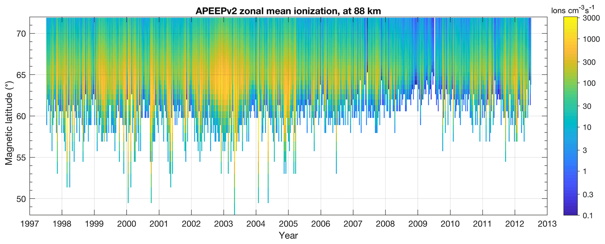
Figure 1Ionization rates from the APEEPv2 model. The daily data have been averaged into 10 d resolution for clarity. The white areas indicate no data and correspond to satellite flux measurements that were screened for being below the noise floor. Tick marks on the x axis are in the middle of each year.
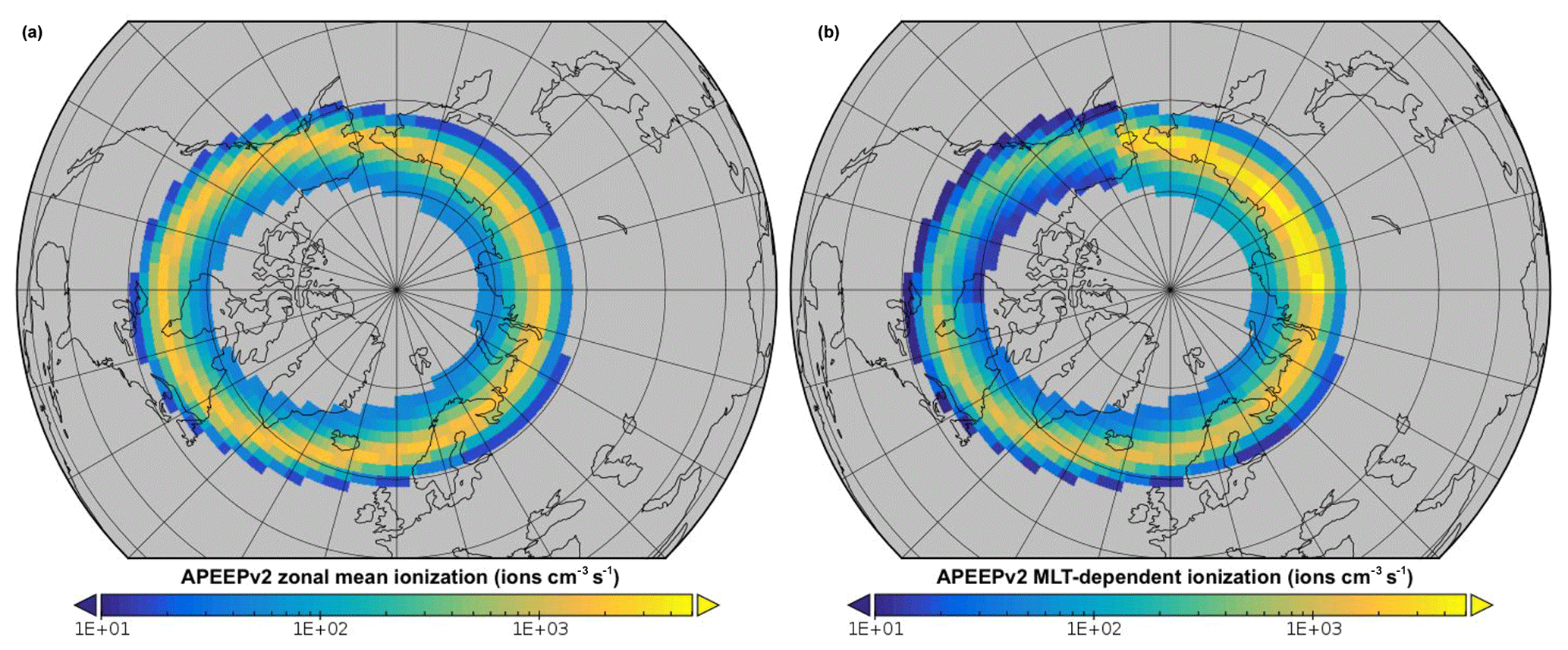
Figure 2Extreme-case ionization rates at an approximative altitude of 75 km (0.0264 hPa) and midnight UT presented on the WACCM-D geographic latitude–longitude grid. (a) APEEPv2 zonal-mean forcing. (b) APEEPv2 MLT-dependent forcing over eight 3 h sectors. Grey areas have no APEEP forcing.
In the CMIP6 EPP data set, the ionization rates due to mid-energy electrons (MEEs) have been calculated using a precipitation model driven by the geomagnetic Ap index (van de Kamp et al., 2016). This model is based on electron flux observations of the Medium-Energy Proton and Electron Detectors (MEPED) flying aboard the Polar-orbiting Operational Environmental Satellites (POES). It provides daily zonal-average ionization rates. Thus, the model neglects the diurnal variation in magnetic local time (MLT) which can be up to several orders of magnitude, e.g. in the MEPED measurements (Horne et al., 2009; Whittaker et al., 2014), and is represented in some particle precipitation models (e.g. AIMOS – Atmospheric Ionization Module OSnabrück; Wissing and Kallenrode, 2009, http://aimos.physik.uos.de, last access: 15 June 2020).
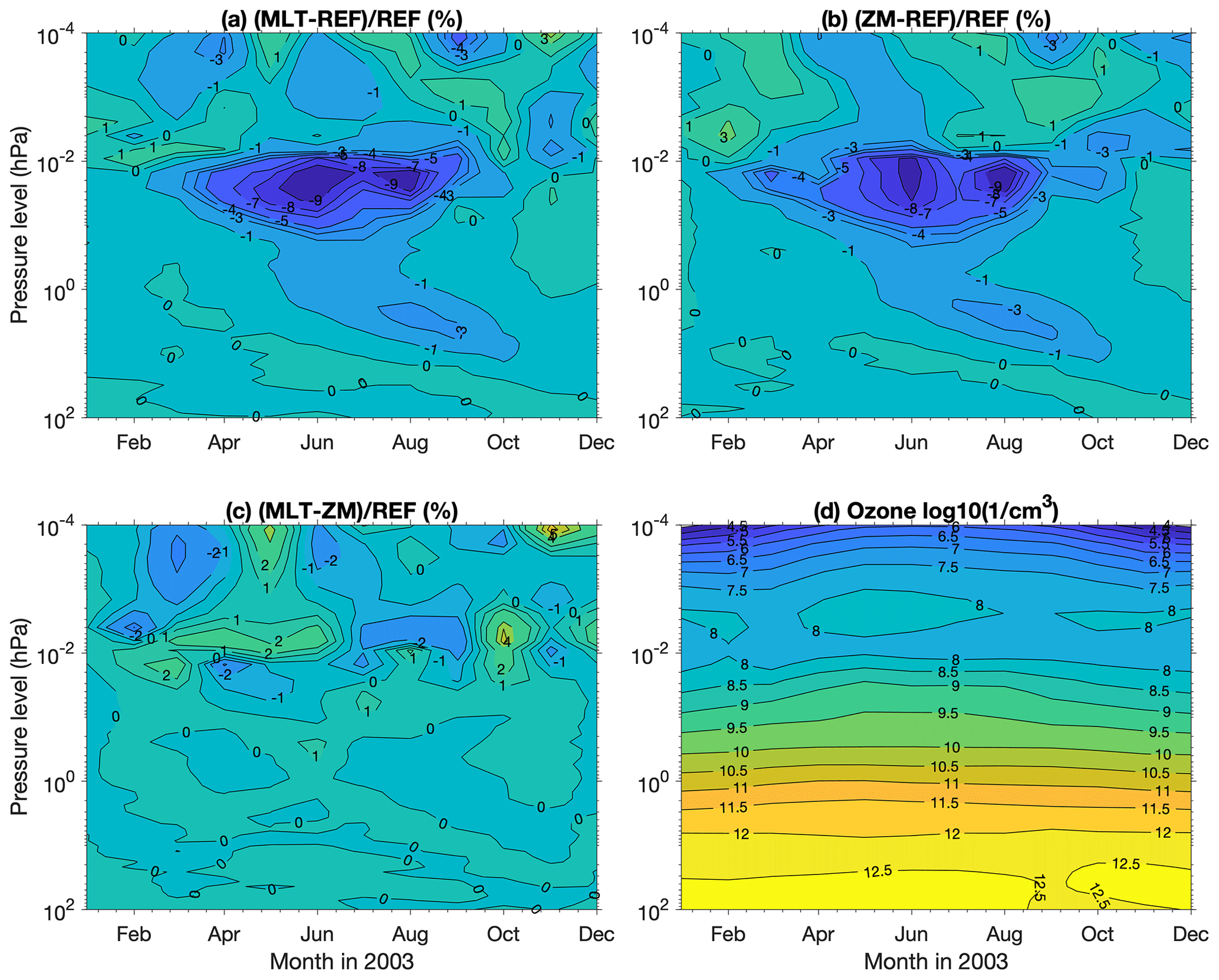
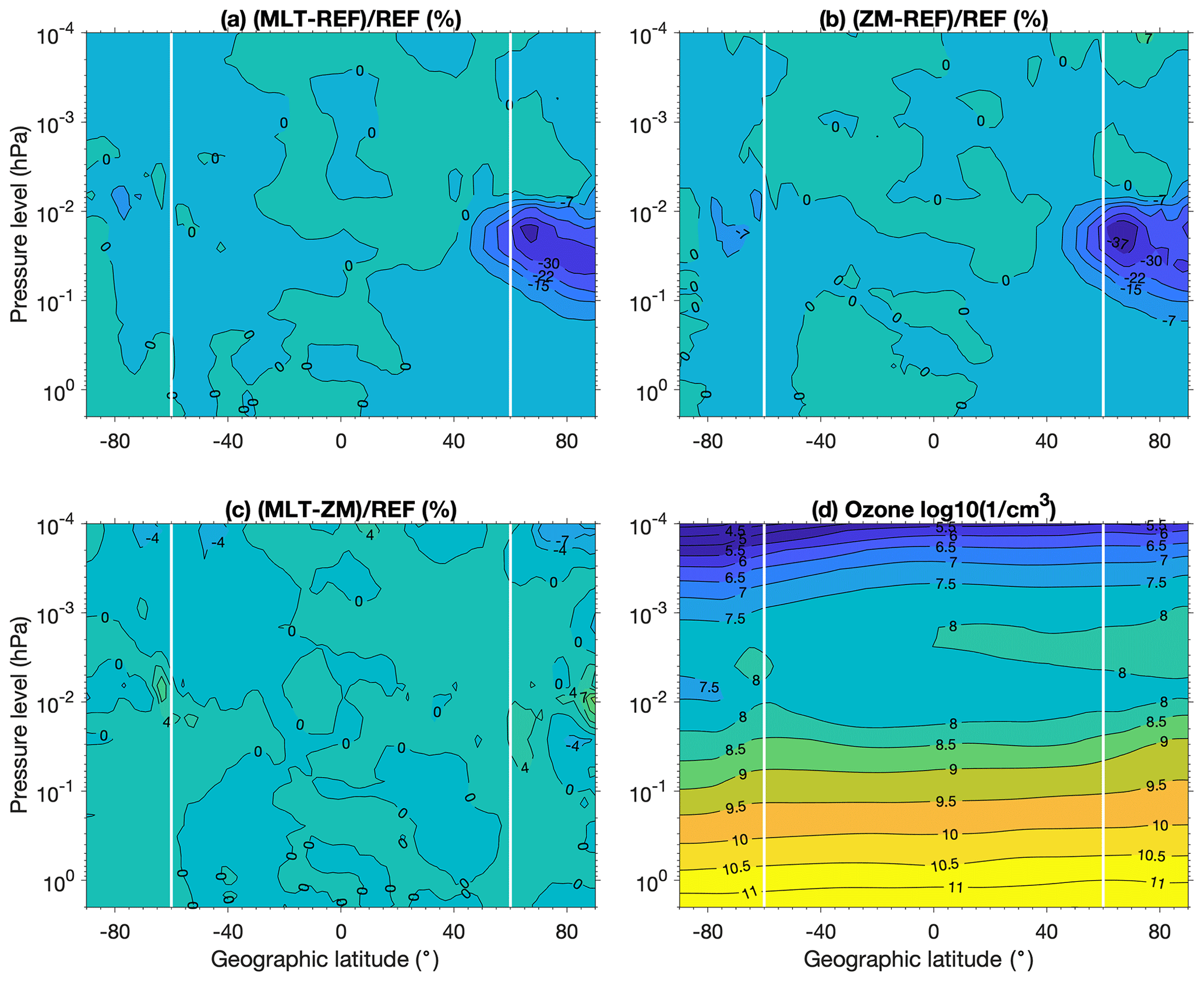
Figure 3Southern Hemisphere (SH) polar-cap ozone monthly means for the year 2003. (a) Relative differences between simulations using MLT-dependent and no MEE forcing. (b) Relative differences between simulations using the zonal mean and no MEE forcing. (c) Relative differences between simulations using MLT-dependent and zonal-mean MEE forcing. (d) Ozone concentration 10-based logarithm from simulations with MLT-dependent MEE.
Due to the energy range used for MEE, i.e. E=30–1000 keV, the bulk of the ionization effects are in the mesosphere at altitudes from 90 to 60 km, corresponding to pressure levels ≈0.001–0.1 hPa (van de Kamp et al., 2016). At these altitudes, EPP causes ionization, production of odd hydrogen (), and HOx-driven catalytic depletion of ozone. Odd nitrogen () is produced and enhanced as well, which can increase the HOx-driven mesospheric ozone depletion by changing the partitioning between HOx species (Verronen and Lehmann, 2015). In polar winter, NOx loss through photodissociation is diminished, and enhanced amounts can be transported from the mesosphere to the stratosphere inside the polar vortex (Callis and Lambeth, 1998; Siskind et al., 2000; Funke et al., 2005; Randall et al., 2009; Päivärinta et al., 2016). This leads to ozone depletion in the upper stratosphere through NOx-driven catalytic loss cycles, typically in late winter and spring (Fytterer et al., 2015; Damiani et al., 2016).
Any MLT dependency in EPP ionization affects the short-term HOx and ozone responses in the mesosphere. The EPP-related HOx production arises from H2O dissociation in reaction sequences forming positive cluster ions, such as H+(H2O), and is also linked to the production of HNO3 through negative-ion chemistry (Verronen and Lehmann, 2013). The HOx production efficiency increases with larger amounts of H2O but decreases with increasing EPP ionization. In addition to HOx, the efficient catalytic loss of ozone requires atomic oxygen which is abundant in the daytime mesosphere. Several studies have reported a diurnal variability in the efficiency of HOx production and magnitude of mesospheric ozone depletion during EPP (Solomon et al., 1981; Aikin and Smith, 1999; Verronen et al., 2005, 2006; Verronen and Lehmann, 2013). The ozone response is dependent on HOx, atomic oxygen, and the electron / negative ion ratio, which have diurnal cycles in the mesosphere.
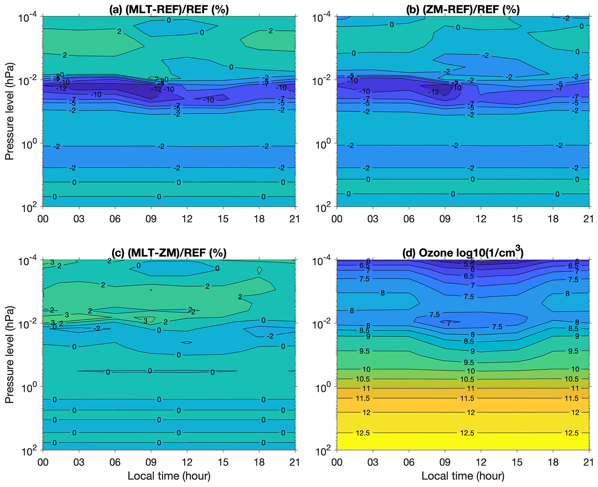
Figure 4Southern Hemisphere (SH) polar-cap ozone. Local-solar-time (LST) means for August 2003. Panels (a)–(d) are as in Fig. 3.
Considering the diurnal variability of ozone depletion reported earlier, it seems clear that the MLT dependency of the MEE forcing must be important if ozone data are analysed at a temporal resolution finer than a day. However, the CMIP6 MEE forcing is intended for multi-decadal climate simulations, which are typically analysed on longer timescales, e.g. as monthly averages. Due to the complexity of factors affecting ozone depletion, it is not clear if results of such an analysis are significantly dependent on the diurnal variability of the EPP forcing. Assessing this would be essential because an accurate representation of middle-atmospheric ozone is crucially needed in climate simulations, e.g. to initiate the dynamical coupling with the troposphere (Andersson et al., 2014).
In this paper, we study the importance of the MLT dependency of the MEE forcing. We do this by comparing atmospheric simulations with daily zonal-mean MEE, i.e. CMIP6 style forcing, to simulations using MLT-dependent MEE. An updated version of the MEE precipitation model includes the dependency on MLT (van de Kamp et al., 2018). The simulations are made with a variant of the Whole Atmosphere Community Climate Model, WACCM-D, which includes mesospheric chemistry of positive and negative ions and is designed for particle precipitation studies in the mesosphere and upper stratosphere (Verronen et al., 2016). WACCM-D allows for detailed simulations of the ion-neutral chemistry interaction leading to HOx production, in contrast to the simple parameterizations that are typically used. We analyse the monthly-mean results as well as the monthly averages at different local times and discuss the differences in the ozone impact in the context of overall uncertainties in the MEE forcing.
Here we use version 1.0.5 of the Community Earth System Model (CESM) with WACCM-D in a similar configuration to that used by Andersson et al. (2016). Version 4 of WACCM is used as described in Marsh et al. (2013). The model was run at latitude × longitude resolution with 88 pressure levels between the ground and the top altitude of hPa (≈140 km). The model is configured in a specified dynamics mode; i.e. surface pressure and horizontal winds and temperatures up to 50 km were constrained to NASA's Modern-Era Retrospective Analysis for Research and Applications (MERRA; Rienecker et al., 2011). The standard EPP input includes precipitation in the auroral regions by electrons with a characteristic energy of 2 keV and a Maxwellian energy distribution as well as ionization due to solar protons at energies between 1 and 300 MeV. In addition, we applied ionization due to galactic cosmic rays (GCRs) from the Nowcast of Atmospheric Ionizing Radiation for Aviation Safety (NAIRAS) model (http://sol.spacenvironment.net/~nairas/, last access: 15 November 2017). Compared to the CMIP6 GCR ionization rates, which are calculated with a Monte Carlo method (Usoskin et al., 2010), NAIRAS ionization rates are about a factor of 2 lower in the stratosphere (Jackman et al., 2016).
For the radiation belt electron precipitation, we used the APEEP (Ap-driven energetic electron precipitation) proxy model version 2 by van de Kamp et al. (2018). Fitted to satellite-based electron observations and using the geomagnetic Ap index as the sole driver, APEEP provides integrated electron fluxes above 30 keV energy and energy-flux gradients at McIlwain L shells between 2 and 10, i.e. between 44 and 72∘ of magnetic latitude. This latitude region is primarily influenced by electrons from the outer Van Allen radiation belt (e.g. Baker et al., 2018). APEEPv2 can output daily zonal averages or daily averages for eight MLT sectors. Compared to the earlier version 1 (van de Kamp et al., 2016), APEEPv2 applies a more conservative noise floor screening for satellite data and provides, in addition to daily zonal means, daily MLT-dependent output over eight 3 h sectors. The purpose of the APEEP models is to allow for multi-decadal climate simulations with electron forcing; e.g. the APEEPv1 atmospheric ionization rates are included in the solar-forcing recommendation of the CMIP6 project, as described in Matthes et al. (2017). For the purpose of this study, the new provision is MLT-dependent MEE ionization production rates. Figure 1 shows ionization rates at 88 km altitude from APEEPv2 for the period between 1998 and 2012. The variation with solar activity is clear, with the lowest ionization seen in 2009 during the solar minimum. The strongest ionization is in the declining phase of the solar cycle, peaking in 2003. The ionization typically maximizes at magnetic latitudes of 60–70∘.
We performed WACCM-D simulations using three different MEE ionization forcings: (1) no MEE (REF; reference), (2) APEEPv2 zonal mean (ZM), and (3) APEEPv2 MLT-dependent (MLT). Note that we calculated APEEPv2 zonal-mean ionization from APEEPv2 MLT ionization to make sure that the daily total energy input is the same for simulations with input 2 and 3. All simulations included the standard aurora and solar-proton-event (SPE) forcing, along with the NAIRAS GCR forcing. Two cases were selected: the year 2003 for high APEEP impact and an extreme case. For the extreme case, high APEEP ionization on 7 March 2005 was first multiplied by a factor of 10 at all altitudes and L shells and then applied constantly in a 3-month simulation from January to March 2002. The extreme case is thus somewhat arbitrary but nevertheless useful for verifying the 2003 results with a very strong and perpetual MEE forcing. The ionization rates for the extreme case are shown in Fig. 2 on the WACCM latitude–longitude grid at an altitude of ≈75 km. MLT is defined as the magnetic longitude from the midnight magnetic meridian, converted to hours at 1 h per 15∘. The difference in forcing between the zonal mean and the MLT-dependent forcing is clear: the MLT ionization is strongest in the early-morning-to-noon sector and has a minimum in the early afternoon. During each 24 h simulation period, these patterns rotate once around the pole, at each time step following MLT. Even at this relatively low altitude, the zonal-mean ionization rate reaches 2000 cm−3 s−1 in the middle of the radiation belt latitudes, while the 2003 mean at the same altitude and latitude is about 65 cm−3 s−1 (not shown).
Obviously, the MLT-dependent forcing produces results that should have differences to those from the ZM forcing if we looked at the hourly output from WACCM-D. This particularly applies to species which have short chemical lifetimes, such as ions. For some neutral species, like HOx, the APEEP-driven differences in production are partly masked by the background diurnal variability of chemical production and loss and are not seen as clearly as in the ionization rates shown in Fig. 2.
However, since the APEEP models are designed to be used in multi-decadal climate simulations such as those conducted during CMIP6, it is more interesting to ask if the analysis of such simulations gives different answers if the MLT-dependent APEEP forcing is applied. Typically, long climate simulations are analysed using monthly-mean data. Thus we concentrate on WACCM-D monthly-mean output first. Then, we also consider different local solar times (LSTs) separately from hourly output data saved separately. This would be similar to the analysis of data from polar-orbiting satellites, since such measurements are typically made at limited local times for any given latitude.
The ozone changes caused by EPP have been suggested to drive the top-down dynamical coupling between the middle atmosphere and the troposphere. Thus we start our analysis directly with ozone and then go on to the ozone-affecting NOx and HOx. The polar-cap means shown in the following sections were calculated as area-weighted (cosine-of-latitude scaling) averages at the geographic latitudes 60–90∘. We concentrate more on the Southern Hemisphere (SH), because there geomagnetic latitudes span over a wider range of geographic latitudes than in the Northern Hemisphere (NH) and thus cover a wider range of background conditions and diurnal variability, especially during winter. Thus we can expect that, overall, the MLT dependency of APEEP forcing should be a more important factor in the SH atmosphere.
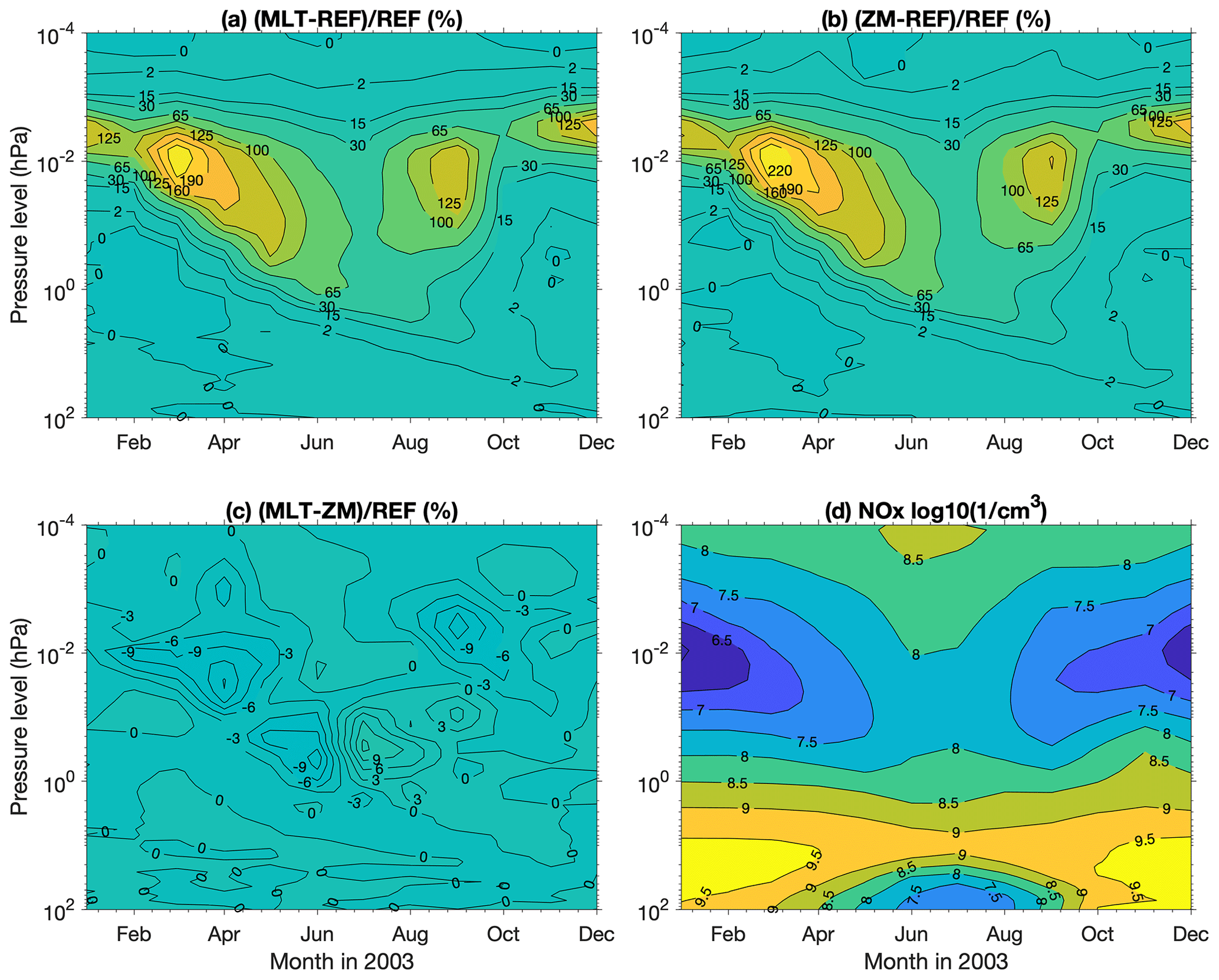
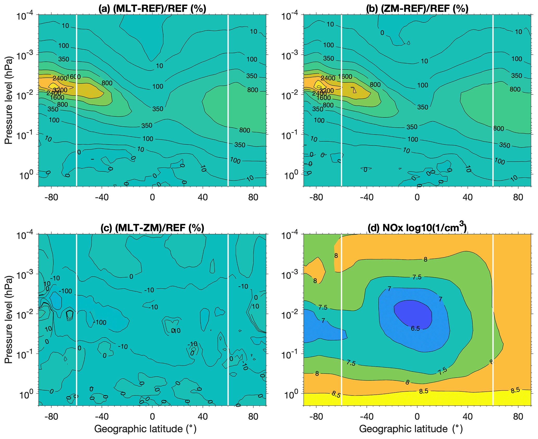
Figure 7Southern Hemisphere (SH) polar-cap NOx, monthly means for year 2003. Panels (a)–(d) are as in Fig. 3.
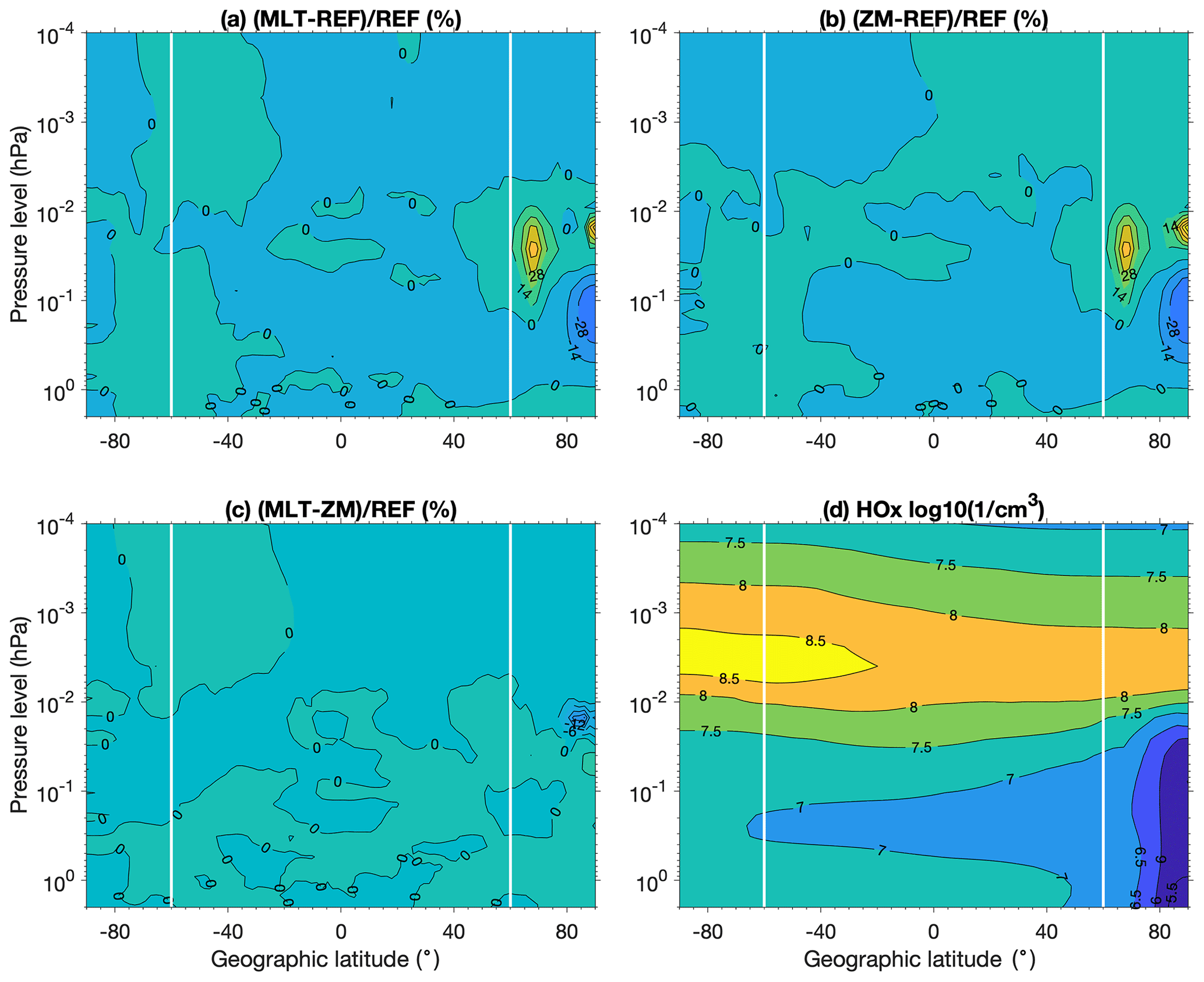
Figure 8February monthly-mean zonal-mean HOx () from the extreme-case simulation. Panels (a)–(d) are as in Fig. 3.
3.1 Ozone
Figure 3 shows the monthly-mean results for the SH polar cap in the year 2003. In Fig. 3a, the impact of MLT-dependent APEEP forcing on mesospheric ozone is strongest, with up to ≈10 % depletion, between April and September at the pressure levels between 0.1 and 0.01 hPa. The depletion is mainly caused by the additional HOx production, with a contribution from the additional NOx production (Verronen and Lehmann, 2015). In the stratosphere, depletion up to ≈3 % is seen from June to October, descending from 1 to 10 hPa. The stratospheric depletion and the descent are both caused by increased NOx descending inside the polar vortex from the production region in the mesosphere–lower thermosphere towards lower altitudes. The APEEP effects are moderate in October and November due to the major effect from the great Halloween solar proton event (e.g. Funke et al., 2011), which is included in all simulations. Above 0.01 hPa, the ozone effect becomes less consistent, i.e. both small increases and decreases are seen, partly due to atomic oxygen changes affecting the total odd-oxygen balance. Overall and qualitatively, our results agree well with mesospheric and stratospheric ozone responses from simulations using free-running dynamics, e.g. with those presented by Andersson et al. (2018).
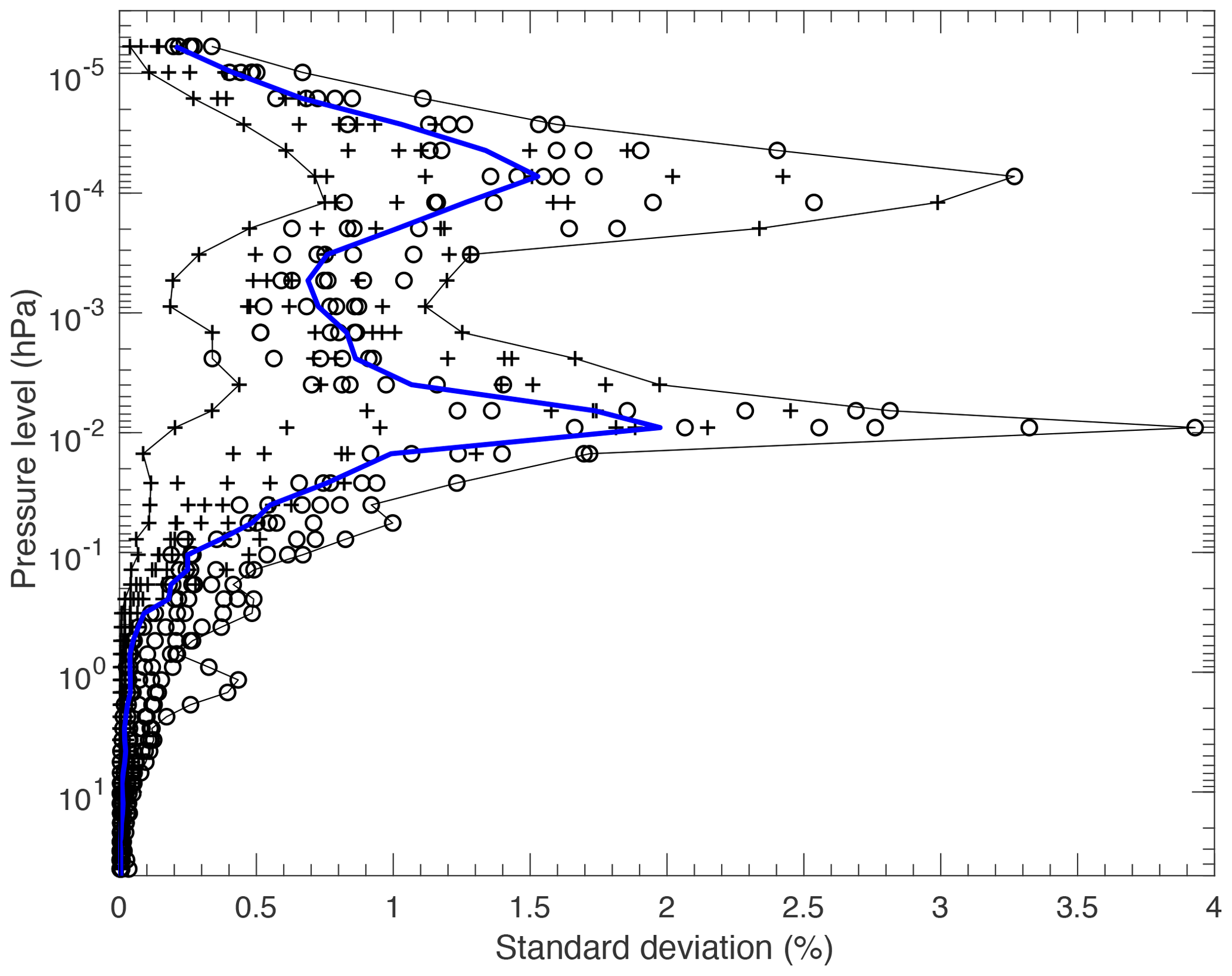
Figure 9Standard deviation (SD) of the Southern Hemisphere (SH) polar-cap monthly ozone anomalies from a 10-member ensemble of SD-WACCM-D APEEP REF simulations, relative to the ensemble mean. Plus signs (+) indicate SDs for the individual months of January, February, March, October, November, and December (summer); circles are for individual months from April to September (winter); black lines are the minimum and maximum SD at each pressure level; and the blue thick line is the median of all monthly SDs.
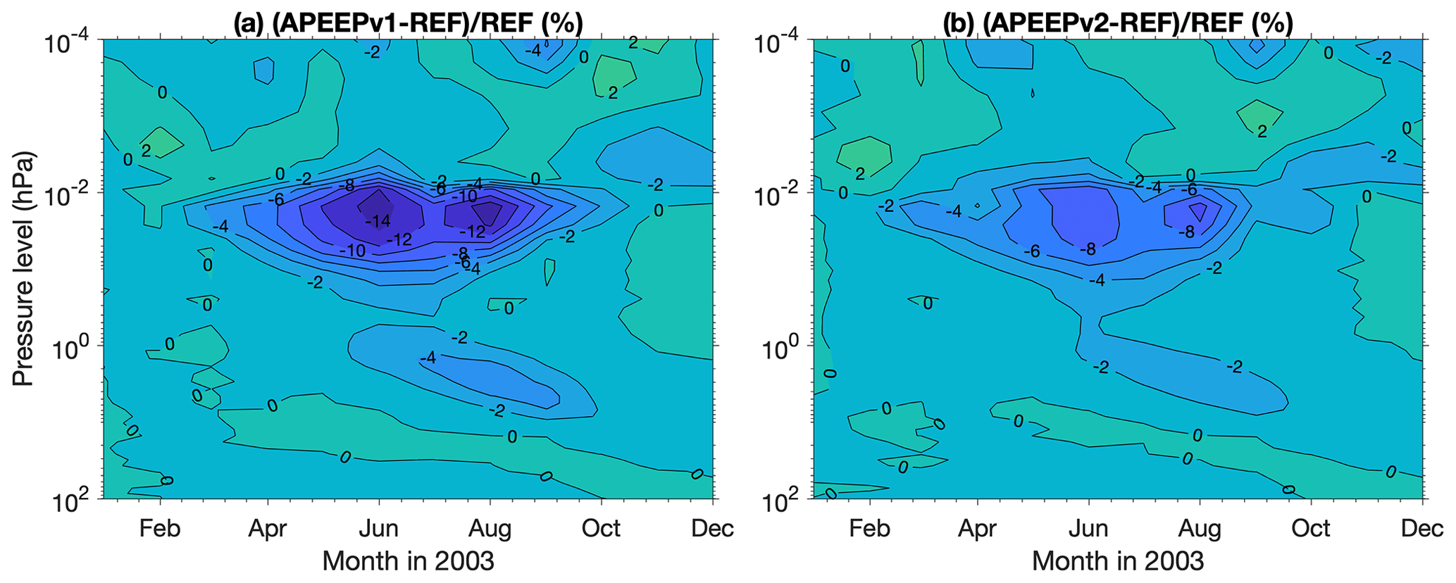
Figure 10Southern Hemisphere (SH) polar-cap ozone monthly means for the year 2003. (a) Relative differences between simulations using APEEPv1 and no MEE forcing. (b) Relative differences between simulations using APEEPv2 and no MEE forcing. Note that panel (b) shows the same data as Fig. 3b, but the contour lines are different.
Figure 3b shows the impact of the ZM APEEP forcing on ozone. The magnitude and extent of the response is clearly very similar to the response caused by the MLT-dependent forcing shown in Fig. 3a. For a more detailed view, Fig. 3c shows the relative difference between simulations using the MLT and the ZM APEEP forcing. The REF simulation (no MEE) is used as a reference here, as it was in panels (a) and (b), so that the percentage numbers in the three panels are directly comparable. The main response patterns below 0.01 hPa in panels (a) and (b) are not seen in panel (c), which indicates that applying MLT dependency has little effect for the monthly-mean ozone impact. Around the 0.01 hPa ozone minimum, there is a region with relative increases and decreases of a few percent.
In the following, we selected August 2003 for a closer study of the effects at different LSTs. As seen in Fig. 3, August has a clear APEEP impact in both the mesosphere and the upper stratosphere. The LST analysis results for other months (not shown) are qualitatively similar to the August results but depend on the overall APEEP impact in each month.
Figure 4 shows the LST mean results for the SH polar cap in August 2003. In other words, the eight LST sectors (3 h each) have been averaged separately over the entire month. Data in each sector are similar to what would be available from satellite instruments which measure at limited local times at each latitude. In Fig. 4a, the impact of APEEP MLT is seen in three altitude stripes across all LSTs. Between 1 and 10 hPa, the depletion of ozone due to descending NOx is not dependent on the LST, and there is no clear diurnal variability of background ozone either (Fig. 4d). From 0.1 to 0.01 hPa, the daytime depletion is at a slightly lower altitude range than at night. However, this is mostly related to the diurnal variability of ozone concentration at these altitudes (Fig. 4d). Around 0.001 hPa, an increase of a few percent is seen especially at nighttime. The increase comes from the production of atomic oxygen, with a lower production from the MLT-dependent forcing at the noon–afternoon sectors. The APEEP contribution is also less important in the daytime when solar extreme-ultraviolet (EUV) radiation dissociates oxygen molecules leading to ozone production.
The response to the ZM APEEP forcing is shown in Fig. 4b, and it is again very similar to the response caused by the MLT-dependent forcing. Figure 4c shows the relative difference between the simulations using the APEEP MLT and the APEEP ZM forcing. Around 0.001 hPa, the MLT forcing depletes 1 %–2 % more ozone than the ZM forcing at all LSTs. This is particularly seen in the early-morning hours when the MLT forcing produces more atomic oxygen compared to the ZM forcing. This effect reaches down to the 0.01 hPa ozone minimum. At 0.1–0.01 hPa, the MLT forcing adds to the ozone depletion by a few percent consistently at all LSTs, which is a minor difference when compared to the 7 %–15 % impact seen in panels (a) and (b) of Fig. 4. Both MLT and ZM forcing produce the largest depletion from midnight to the early morning. In the stratosphere, the differences are less than 1 %.
Figure 5 shows an example of our results from the extreme case; the data shown are monthly zonal means for February. Here we look at the MEE forcing region only, i.e. in the mesosphere and above, because the 3-month span of this simulation is not long enough for the NOx transport to cause full stratospheric effects. The ozone impacts below 0.1 hPa are thus small (not shown). Although both hemispheres were equally forced with APEEP, except for the differences in the geographic extent of magnetic latitudes, the ozone effect is much clearer over the NH winter pole (Fig. 5a and b) due to a faster recovery in the summer pole through production driven by O2 photodissociation. Depletion is seen at an altitude range between 0.01 and 0.5 hPa at the latitudes poleward of 45∘, with the strongest effect reaching 45 % just below 0.01 hPa and north of 60∘. The depletion here is naturally stronger than for the year 2003 because the extreme APEEP forcing was applied throughout the simulation. The response extends down to latitude, which is consistent with the extent of the APEEP forcing (see Fig. 2). The simulations with the ZM and the MLT forcings give very similar results, and the differences are generally marginal in the range of a few percent, except in a few small and isolated regions.
3.2 Odd nitrogen
The chemical lifetime of odd nitrogen (NOx) is days to months in the mesosphere–lower thermosphere, and its concentration can easily accumulate especially during polar winter conditions. Therefore, one would expect that a faithful representation of the MLT dependency of the APEEP forcing and the related NOx production is probably not crucial for the NOx distribution or the NOx-driven ozone depletion in the upper stratosphere.
Figure 6 shows the monthly zonal-mean results for February from the extreme case. The largest increases, reaching up to and beyond an order of magnitude, are seen between 0.1 and 0.001 hPa at the polar latitudes, i.e. at the latitudes and altitudes where the APEEP forcing is applied. The increase extends from the polar regions to all latitudes, with the mid and low latitudes outside the forcing region showing a smaller but still >100 % impact in large regions. The SH effect is relatively stronger in magnitude than the NH effect due to the lower background concentration there. In the NH, the beginning effect of NOx descent inside the polar vortex extends the impact towards the stratopause. The MLT and the ZM forcings again produce a very similar response in both magnitude and spatial extent, with the differences being small compared to the overall effect. However, the MLT forcing results in up to 1∕10 less NOx in the peak response regions around 0.01 hPa than the ZM forcing, except above the 80 ∘ latitudes at the poles. At the pressure levels below 0.05 hPa and above 0.003 hPa the relative differences are smaller.
Figure 7 shows the monthly-mean results for the SH polar cap in the year 2003. In the summer months, the APEEP forcing enhances NOx down to the middle mesosphere only, due to the lack of downward transport combined with the efficient loss from solar photodissociation. During the winter months, when less radiation is available and the chemical lifetime of NOx increases, NOx created by APEEP above 0.1 hPa descends inside the polar vortex towards the stratospheric altitudes. Relatively, the NOx enhancement is strongest during the autumn and spring, due to a combination of lower solar photodissociation and lower background concentration than in the summer and winter, respectively. The results we show in Fig. 7 agree qualitatively well with the season-dependent NOx responses from WACCM simulations using free-running dynamics (e.g. Andersson et al., 2018). The differences between the response to APEEP MLT and ZM are rather small. In general, the differences in the resulting NOx concentration are less than 1∕10, except in July around 0.2 hPa. In the autumn and early winter, the MLT forcing results in a smaller NOx response in the mesosphere compared to the ZM forcing, while in the late winter the MLT forcing produces more NOx in the lower mesosphere.
3.3 Odd hydrogen
The odd-hydrogen (HOx) production from H2O by the APEEP ionization is restricted to the altitudes below 0.01 hPa (≈80 km), due to the small amount of H2O available for ion chemistry at the altitudes above. This is clearly seen in Fig. 8a, which shows the monthly zonal-mean response to APEEP MLT for February from the extreme case: there is no clear response above 0.01 hPa at any latitude. Also, the SH summer pole shows little effect due to the APEEP contribution being less than that from the solar Lyman-α photodissociation of H2O. In the NH winter pole, the largest region of HOx increase is at 0.1–0.01 hPa and at the latitudes between 40 and 80∘, i.e. exactly in the region of direct APEEP forcing. In contrast, a clear decrease is seen below 0.04 hPa at the high latitudes above 80∘, in a region where the HOx background concentration is very small. This happens outside the APEEP HOx production region and seems to be a chemical response to enhanced NOx, similar to the decrease in HOx at 45–60 km shown by Verronen and Lehmann (2015) in their Fig. 1.
Our results indicate that the MLT-dependent diurnal variability of MEE forcing can be ignored without causing large differences in simulated ozone responses on monthly timescales. The same conclusion applies to monthly averages calculated at individual local times. When comparing the simulations using a daily zonal-average MEE and an MLT-dependent MEE, differences in the magnitude of the response do exist, but they are not more than a few percent for ozone. The spatial patterns of response are very similar between the simulations. Thus, the lack of MLT dependency in the current CMIP6 MEE forcing data should not create any important uncertainty in long-term climate simulations.
Our simulations use the MERRA-specified dynamics up to 50 km altitude. In the stratosphere, the small chemical differences between the simulations suggest that any differences in dynamics or dynamical feedback would also be small. Above 50 km, our simulations are dynamically free running. In general, the specified dynamics below 50 km control much of the dynamics at altitudes above as well. Thus, dynamical differences between simulations using specified dynamics should be much smaller than between fully free-running simulations. Nevertheless, as seen in Fig. 3c for ozone, the relative differences between the APEEP MLT and the APEEP ZM simulations above 0.1 hPa (≈60 km) increase from <1 % to up to 2 %–4 % around 0.01 hPa, are smaller around 0.001 hPa, and then increase again around 0.0001 hPa. Although part of this increase in relative differences comes from the smaller background values of ozone than at the altitudes below (see Fig. 3d), there should also be a contribution from the free-running dynamics. To quantify this contribution, we performed a 10-member ensemble of simulations for the year 2003, with specified dynamics and no MEE forcing. From this ensemble, we calculated the standard deviation of monthly-mean polar-cap anomalies (N=10), individually for each month, and show them for the SH in Fig. 9. Below 0.1 hPa, i.e. at the altitudes where the specified dynamics are applied, SD is always below 0.5 %. Above, there are two SD maxima around 0.01 and 0.0001 hPa, on average 1.5 %–2 % and reaching up to 3 %–4 % in the winter months. These maxima coincide with the increased ozone differences seen in Fig. 3c and have a similar magnitude. Thus the ozone differences between simulations, seen when using different MLT dependencies for the applied APEEP forcing, are within the statistical variability coming from the free-running model dynamics and are not significant.
To put the uncertainties caused by the MEE MLT dependency into a wider context, Fig. 10 shows a SH ozone impact comparison between simulations using a zonal-mean forcing from APEEPv1 and APEEPv2 for the year 2003. The ozone impact from APEEPv1 is, in general, about twice as large as that from APEEPv2. This is seen for the mesospheric HOx-driven depletion in midwinter as well as for the springtime NOx-driven depletion in the upper stratosphere. The difference in ozone impact is a result of the lower ionization rates in APEEPv2, caused by a more careful consideration of the MEPED instrument noise floor (van de Kamp et al., 2018). Further, recent studies have demonstrated that the uncertainties related to the MEPED electron flux measurements, which the APEEP models are based on, can reach an order of magnitude in certain conditions and particularly when fluxes are low (Nesse Tyssøy et al., 2019). Thus it seems clear that the impact of uncertainties related to the electron flux observations greatly exceeds those related to the MLT dependency applied in atmosphere and climate simulations.
We conclude that for the monthly-mean atmospheric impact caused by MEE that ignoring the MLT dependency does not create significant differences in simulations. This does not apply for atmospheric impacts in daily or hourly timescales, which should be studied separately. Finally, it is important to note that good MLT coverage is a crucial factor when making MEE flux observations because of the order-of-magnitude variability with MLT (e.g. in Fig. 2). Even when atmospheric simulations can be made with a zonal-mean MEE forcing, it is important to apply a forcing that provides the correct total amount of energy input, and this requires flux measurements that have an adequate MLT coverage. Nevertheless, the assessment of ozone and NOx responses does not need a complete MLT coverage, which eases the observational requirements for any new atmospheric instrument or existing data sets.
All model data used are available from the corresponding author upon request (pekka.verronen@oulu.fi). CESM source code is distributed freely through a public Subversion code repository (http://www.cesm.ucar.edu/models/cesm1.0/, last access: 7 July 2020). WACCM-D was officially released with CESM version 2.0 in June 2018 (http://www.cesm.ucar.edu/models/cesm2/, last access: 7 July 2020). The APEEP ionization data sets are available from the CHAMOS web page (http://chamos.fmi.fi/chamos_apeep.html, last access: 9 July 2020) and the SOLARIS-HEPPA web page (https://solarisheppa.geomar.de/cmip6, last access: 9 July 2020), see also van de Kamp et al. (2016, 2018).
PTV and DRM planned the research and prepared the model and the simulations with input from MES and NK. PTV carried out the simulations and the analysis and led the writing of the paper. All authors contributed to the discussion and the writing of the final paper.
The authors declare that they have no conflict of interest.
The authors would like to thank the CHAMOS group (http://chamos.fmi.fi) for useful discussions. This material is based upon work supported in part by the National Center for Atmospheric Research, which is a major facility sponsored by the National Science Foundation (cooperative agreement no. 1852977). Daniel R. Marsh is also supported by an NSF award for “Collaborative Research: CEDAR – Quantifying the Impact of Radiation Belt Electron Precipitation on Atmospheric Reactive Nitrogen Oxides (NOx) and Ozone (O3)” (no. 1650918).
This research has been supported by a National Science Foundation award for “Collaborative Research: CEDAR – Quantifying the Impact of Radiation Belt Electron Precipitation on Atmospheric Reactive Nitrogen Oxides (NOx) and Ozone (O3)” (grant no. 1650918).
This paper was edited by Gunter Stober and reviewed by two anonymous referees.
Aikin, A. C. and Smith, H. J. P.: Mesospheric constituent variations during electron precipitation events, J. Geophys. Res., 104, 26457–26472, 1999. a
Andersson, M. E., Verronen, P. T., Rodger, C. J., Clilverd, M. A., and Seppälä, A.: Missing driver in the Sun-Earth connection from energetic electron precipitation impacts mesospheric ozone, Nat. Commun., 5, 5197, https://doi.org/10.1038/ncomms6197, 2014. a, b
Andersson, M. E., Verronen, P. T., Marsh, D. R., Päivärinta, S.-M., and Plane, J. M. C.: WACCM-D – Improved modeling of nitric acid and active chlorine during energetic particle precipitation, J. Geophys. Res.-Atmos., 121, 10328–10341, https://doi.org/10.1002/2015JD024173, 2016. a
Andersson, M. E., Verronen, P. T., Marsh, D. R., Seppälä, A., Päivärinta, S.-M., Rodger, C. J., Clilverd, M. A., Kalakoski, N., and van de Kamp, M.: Polar Ozone Response to Energetic Particle Precipitation Over Decadal Time Scales: The Role of Medium-Energy Electrons, J. Geophys. Res.-Atmos., 123, 607–622, https://doi.org/10.1002/2017JD027605, 2018. a, b
Baker, D. N., Erickson, P. J., Fennell, J. F., Foster, J. C., Jaynes, A. N., and Verronen, P. T.: Space weather effects in the Earth's radiation belts, Space Sci. Rev., 214, 17, https://doi.org/10.1007/s11214-017-0452-7, 2018. a
Callis, L. B. and Lambeth, J. D.: NOy formed by precipitating electron events in 1991 and 1992: Descent into the stratosphere as observed by ISAMS, Geophys. Res. Lett., 25, 1875–1878, https://doi.org/10.1029/98GL01219, 1998. a
Damiani, A., Funke, B., Santee, M. L., Cordero, R. R., and Watanabe, S.: Energetic particle precipitation: A major driver of the ozone budget in the Antarctic upper stratosphere, Geophys. Res. Lett., 43, 3554–3562, https://doi.org/10.1002/2016GL068279, 2016. a
Funke, B., López-Puertas, M., Gil-Lopez, S., von Clarmann, T., Stiller, G. P., Fischer, H., and Kellmann: Downward transport of upper atmospheric NOx into the polar stratosphere and lower mesosphere during the Antarctic 2003 and Arctic 2002/2003 winters, J. Geophys. Res., 110, D24308, https://doi.org/10.1029/2005JD006463, 2005. a
Funke, B., Baumgaertner, A., Calisto, M., Egorova, T., Jackman, C. H., Kieser, J., Krivolutsky, A., López-Puertas, M., Marsh, D. R., Reddmann, T., Rozanov, E., Salmi, S.-M., Sinnhuber, M., Stiller, G. P., Verronen, P. T., Versick, S., von Clarmann, T., Vyushkova, T. Y., Wieters, N., and Wissing, J. M.: Composition changes after the “Halloween” solar proton event: the High Energy Particle Precipitation in the Atmosphere (HEPPA) model versus MIPAS data intercomparison study, Atmos. Chem. Phys., 11, 9089–9139, https://doi.org/10.5194/acp-11-9089-2011, 2011. a
Fytterer, T., Mlynczak, M. G., Nieder, H., Pérot, K., Sinnhuber, M., Stiller, G., and Urban, J.: Energetic particle induced intra-seasonal variability of ozone inside the Antarctic polar vortex observed in satellite data, Atmos. Chem. Phys., 15, 3327–3338, https://doi.org/10.5194/acp-15-3327-2015, 2015. a
Horne, R. B., Lam, M. M., and Green, J. C.: Energetic electron precipitation from the outer radiation belt during geomagnetic storms, Geophys. Res. Lett., 36, L19104, https://doi.org/10.1029/2009GL040236, 2009. a
Jackman, C. H., Marsh, D. R., Kinnison, D. E., Mertens, C. J., and Fleming, E. L.: Atmospheric changes caused by galactic cosmic rays over the period 1960–2010, Atmos. Chem. Phys., 16, 5853–5866, https://doi.org/10.5194/acp-16-5853-2016, 2016. a
Marsh, D. R., Mills, M., Kinnison, D., Lamarque, J.-F., Calvo, N., and Polvani, L.: Climate change from 1850 to 2005 simulated in CESM1(WACCM), J. Clim., 26, 7372–7391, https://doi.org/10.1175/JCLI-D-12-00558.1, 2013. a
Matthes, K., Funke, B., Andersson, M. E., Barnard, L., Beer, J., Charbonneau, P., Clilverd, M. A., Dudok de Wit, T., Haberreiter, M., Hendry, A., Jackman, C. H., Kretschmar, M., Kruschke, T., Kunze, M., Langematz, U., Marsh, D. R., Maycock, A., Misios, S., Rodger, C. J., Scaife, A. A., Seppälä, A., Shangguan, M., Sinnhuber, M., Tourpali, K., Usoskin, I., van de Kamp, M., Verronen, P. T., and Versick, S.: Solar Forcing for CMIP6, Geosci. Model Dev., 10, 2247–2302, https://doi.org/10.5194/gmd-10-2247-2017, 2017. a, b
Nesse Tyssøy, H., Haderlein, A., Sandanger, M. I., and Stadsnes, J.: Intercomparison of the POES/MEPED loss cone electron fluxes with the CMIP6 parametrization, J. Geophys. Res.-Space, 124, 628–642, https://doi.org/10.1029/2018JA025745, 2019. a
Päivärinta, S.-M., Verronen, P. T., Funke, B., Gardini, A., Seppälä, A., and Andersson, M. E.: Transport versus energetic particle precipitation: Northern polar stratospheric NOx and ozone in January–March 2012, J. Geophys. Res.-Atmos., 121, 6085–6100, https://doi.org/10.1002/2015JD024217, 2016. a
Randall, C. E., Harvey, V. L., Siskind, D. E., France, J., Bernath, P. F., Boone, C. D., and Walker, K. A.: NOx descent in the Arctic middle atmosphere in early 2009, Geophys. Res. Lett., 36, L18811, https://doi.org/10.1029/2009GL039706, 2009. a
Rienecker, M. M., Suarez, M. J., Gelaro, R., Todling, R., Bacmeister, J., Liu, E., Bosilovich, M. G., Schubert, S. D., Takacs, L., Kim, G.-K., Bloom, S., Chen, J., Collins, D., Conaty, A., da Silva, A., Gu, W., Joiner, J., Koster, R. D., Lucchesi, R., Molod, A., Owens, T., Pawson, S., Pegion, P., Redder, C. R., Reichle, R., Robertson, F. R., Ruddick, A. G., Sienkiewicz, M., and Woollen, J.: MERRA: NASA's Modern-Era Retrospective Analysis for Research and Applications, J. Clim., 24, 3624–3648, https://doi.org/10.1175/JCLI-D-11-00015.1, 2011. a
Siskind, D. E., Nedoluha, G. E., Randall, C. E., Fromm, M., and Russell III, J. M.: An assessment of Southern Hemisphere stratospheric NOx enhancements due to transport from the upper atmosphere, Geophys. Res. Lett., 27, 329–332, 2000. a
Solomon, S., Rusch, D. W., Gérard, J.-C., Reid, G. C., and Crutzen, P. J.: The effect of particle precipitation events on the neutral and ion chemistry of the middle atmosphere: II. Odd hydrogen, Planet. Space Sci., 8, 885–893, 1981. a
Usoskin, I. G., Kovaltsov, G. A., and Mironova, I. A.: Cosmic ray induced ionization model CRAC : CRII: An extension to the upper atmosphere, J. Geophys. Res.-Atmos., 115, D10302, https://doi.org/10.1029/2009JD013142, 2010. a
van de Kamp, M., Seppälä, A., Clilverd, M. A., Rodger, C. J., Verronen, P. T., and Whittaker, I. C.: A model providing long-term datasets of energetic electron precipitation during geomagnetic storms, J. Geophys. Res.-Atmos., 121, 12520–12540, https://doi.org/10.1002/2015JD024212, 2016. a, b, c, d
van de Kamp, M., Rodger, C. J., Seppälä, A., Clilverd, M. A., and Verronen, P. T.: An updated model providing long-term datasets of energetic electron precipitation, including zonal dependence, J. Geophys. Res.-Atmos., 123, 9891–9915, https://doi.org/10.1029/2017JD028253, 2018. a, b, c, d
Verronen, P. T. and Lehmann, R.: Analysis and parameterisation of ionic reactions affecting middle atmospheric HOx and NOy during solar proton events, Ann. Geophys., 31, 909–956, https://doi.org/10.5194/angeo-31-909-2013, 2013. a, b
Verronen, P. T. and Lehmann, R.: Enhancement of odd nitrogen modifies mesospheric ozone chemistry during polar winter, Geophys. Res. Lett., 42, 10445–10452, https://doi.org/10.1002/2015GL066703, 2015. a, b, c
Verronen, P. T., Seppälä, A., Clilverd, M. A., Rodger, C. J., Kyrölä, E., Enell, C.-F., Ulich, T., and Turunen, E.: Diurnal variation of ozone depletion during the October-November 2003 solar proton events, J. Geophys. Res., 110, A09S32, https://doi.org/10.1029/2004JA010932, 2005. a
Verronen, P. T., Seppälä, A., Kyrölä, E., Tamminen, J., Pickett, H. M., and Turunen, E.: Production of odd hydrogen in the mesosphere during the January 2005 solar proton event, Geophys. Res. Lett., 33, L24811, https://doi.org/10.1029/2006GL028115, 2006. a
Verronen, P. T., Andersson, M. E., Marsh, D. R., Kovács, T., and Plane, J. M. C.: WACCM-D – Whole Atmosphere Community Climate Model with D-region ion chemistry, J. Adv. Model. Earth Syst., 8, 954–975, https://doi.org/10.1002/2015MS000592, 2016. a
Whittaker, I. C., Clilverd, M. A., and Rodger, C. J.: Characteristics of precipitating energetic electron fluxes relative to the plasmapause during geomagnetic storms, J. Geophys. Res.-Space Phys., 119, 8784–8800, https://doi.org/10.1002/2014JA020446, 2014. a
Wissing, J. M. and Kallenrode, M.-B.: Atmospheric Ionization Module Osnabrück (AIMOS): A 3-D model to determine atmospheric ionization by energetic charged particles from different populations, J. Geophys. Res., 114, A06104, https://doi.org/10.1029/2008JA013884, 2009. a