the Creative Commons Attribution 4.0 License.
the Creative Commons Attribution 4.0 License.
 | 16 Jun 2020
Comparison of quiet-time ionospheric total electron content from the IRI-2016 model and from gridded and station-level GPS observations
Gizaw Mengistu Tsidu
Mulugeta Melaku Zegeye
Earth's ionosphere is an important medium of radio wave propagation in modern times. However, the effective use of the ionosphere depends on the understanding of its spatiotemporal variability. Towards this end, a number of ground- and space-based monitoring facilities have been set up over the years. The information from these stations has also been complemented by model-based studies. However, assessment of the performance of ionospheric models in capturing observations needs to be conducted. In this work, the performance of the IRI-2016 model in simulating the total electron content (TEC) observed by a network of Global Positioning System (GPS) receivers is evaluated based on the RMSE, the bias, the mean absolute error (MAE) and skill score, the normalized mean bias factor (NMBF), the normalized mean absolute error factor (NMAEF), the correlation, and categorical metrics such as the quantile probability of detection (QPOD), the quantile categorical miss (QCM), and the quantile critical success index (QCSI). The IRI-2016 model simulations are evaluated against gridded International Global Navigation Satellite System (GNSS) Service (IGS) GPS-TEC and TEC observations at a network of GPS receiver stations during the solar minima in 2008 and solar maxima in 2013. The phases of modeled and simulated TEC time series agree strongly over most of the globe, as indicated by a high correlations during all solar activities with the exception of the polar regions. In addition, lower RMSE, MAE, and bias values are observed between the modeled and measured TEC values during the solar minima than during the solar maxima from both sets of observations. The model performance is also found to vary with season, longitude, solar zenith angle, and magnetic local time. These variations in the model skill arise from differences between seasons with respect to solar irradiance, the direction of neutral meridional winds, neutral composition, and the longitudinal dependence of tidally induced wave number four structures. Moreover, the variation in model performance as a function of solar zenith angle and magnetic local time might be linked to the accuracy of the ionospheric parameters used to characterize both the bottom- and topside ionospheres. However, when the NMBF and NMAEF are applied to the data sets from the two distinct solar activity periods, the difference in the skill of the model during the two periods decreases, suggesting that the traditional model evaluation metrics exaggerate the difference in model skill. Moreover, the performance of the model in capturing the highest ends of extreme values over the geomagnetic equator, midlatitudes, and high latitudes is poor, as noted from the decrease in the QPOD and QCSI as well as an increase in the QCM over most of the globe with an increase in the threshold percentile TEC values from 10 % to 90 % during both the solar minimum and the solar maximum periods. The performance of IRI-2016 in simulating observed low (as low as the 10th percentile) and high (higher than the 90th percentile) TEC correctly over equatorial ionization anomaly (EIA) crest regions is reasonably good given that IRI-2016 is a climatological model. However, it is worth noting that the performance of the IRI-2016 model is relatively poor in 2013 compared with 2008 at the highest ends of the TEC distribution. Therefore, this study reveals the strengths and weaknesses of the IRI-2016 model in simulating the observed TEC distribution correctly during all seasons and solar activities for the first time.
- Article
(15210 KB) - Full-text XML
- BibTeX
- EndNote


Radio waves have become an indispensable and spectacular tool in the progress of space satellite communication and navigation, and the Earth's ionosphere is an essential medium for the propagation of radio wave signals (Mengistu Tsidu and Abraha, 2014, and references therein). As a result, Kumar et al. (2014) noted that dual-frequency Global Positioning System (GPS) receivers have increased worldwide, and numerous networks now exist in order to enhance applications based on space satellite communications and navigation. However GPS signals are influenced by ionospheric disturbances due to the existence of electrons. The total electron content (TEC) is a parameter that provides a complete picture of the ionosphere. It is an essential ionospheric property for the investigation of ionospheric variability and dynamics, as the TEC changes as a function of geographic location, time of the day, day of the season, season of the year, and solar and geomagnetic activity. As a result, several authors have investigated the distribution and characteristics of TEC variations (Mukherjee et al., 2010; Sethi et al., 2011; Mengistu Tsidu and Abraha, 2014; Bardhan et al., 2014; Saranya et al., 2014; Grynyshyna-Poliuga et al., 2015; Themens and Jayachandran, 2016; Sharma et al., 2017; Venkata Ratnam et al., 2017; Perna et al., 2017; Rao et al., 2018; Perna et al., 2018). Moreover, the coupling of the lower atmosphere and ionosphere as well as the coupling of the thermosphere and magnetosphere contribute to the complexity of TEC variability in the ionosphere (Oberheide and Gusev, 2002; Takahashi et al., 2005, 2006, 2007, 2009; Lühr et al., 2007; Wu et al., 2009; Liu et al., 2010; Onohara et al., 2013; Mengistu Tsidu and Abraha, 2014; Fekadu et al., 2019). Understanding TEC variability allows us to characterize the time delay in radio wave signals induced by the ionosphere, as the delay is directly proportional to the TEC, and to develop ionospheric models for TEC prediction.
Historically, as an early part of efforts to understand the Earth's upper ionosphere, the first satellites' radio measurements recorded some crucial results with respect to the upper atmosphere. Measurements of the orbital period using radio locations revealed that temperature and density show high discrepancies in the upper atmosphere (Bilitza et al., 1990). The decision was made by the formerly established Committee on Space Research (COSPAR) to develop a set of empirically based tables expressing these new results. Thus, the new results have been presented using the name “COSPAR International Reference Atmosphere” (CIRA) since 1961. A few years later, following the establishment of CIRA, Sidney Bowhill proposed a reference that was named “International Reference Ionosphere” (IRI) to represent the ionized constituents of the atmosphere (Rawer et al., 1978; Bilitza, 1986; Rawer, 1988; Bilitza et al., 1990). The International Union of Radio Science (URSI) begun to cooperate with COSPAR on the IRI in 1969. Thus, the IRI models are managed by COSPAR and URSI.
IRI, one of the empirical modeling tools currently available to the wider scientific community, portrays the spatial and temporal variability of the ionosphere for a specific solar variability (Bilitza et al., 1990, 2014; Bilitza, 2001). IRI may forecast monthly TEC variability better than TEC daily variability, as the IRI model is a climatological model and its parameters are derived based on the availability of ground, in situ, and space-based measurements. Therefore, IRI is globally recognized as the guideline for ionospheric parameters and has been applied by various scholars in comparison studies with TEC derived from GNSS GPS networks and in other studies (Kouris and Fotiadis, 2002; Kouris et al., 2004; Zhang et al., 2006; Mukherjee et al., 2010; Sethi et al., 2011; Bilitza et al., 2011; Bardhan et al., 2014; Yekoye et al., 2014; Saranya et al., 2014; Grynyshyna-Poliuga et al., 2015; Mengistu Tsidu et al., 2016; Wang et al., 2016; Themens and Jayachandran, 2016; Perna et al., 2017; Venkata Ratnam et al., 2017; Sharma et al., 2017; Perna et al., 2018; Rao et al., 2018). For instance, in the older model versions (IRI-2000 and IRI-2001), it was found that IRI overestimates both ionogram and GPS-TEC values (Mosert et al., 2007). Praveen et al. (2010) found that the estimations of the IRI-2007 model have seasonal and longitudinal discrepancies in TEC over low-latitude stations. Kenpankho et al. (2011) also noted that IRI-2007 underestimates GPS-TEC over an equatorial region in Thailand with poorer performance during the day than at night. Venkata Ratnam et al. (2017) found that the IRI-2007 and IRI-2012 models capture observed GPS-TEC at two low-latitude GPS stations in India except during the dawn hours (01:00–06:00 LT) when the models overestimate TEC. The authors also revealed the presence of higher percentage deviations during the equinoctial months than in summer. Moreover, the authors noted the limited skill of the models in capturing observed TEC changes during a June storm in 2013, although there was some difference between the two versions of the model. In fact, the poor skill of IRI in simulating TEC during geomagnetic storms has also been reported by numerous other authors (e.g., Yekoye et al., 2014; Tariku, 2015). The weaknesses of IRI-2012 are not only limited to storm events. Kumar (2016) determined that the performance of IRI-2012 in simulating TEC over the global equatorial region is better during a deep solar minimum (2009) than a solar maximum year (2012), as the IRI-2012 model overestimates the observed GPS-TEC at all equatorial stations with a larger discrepancy with respect to observations during a solar maximum (2012) than during a solar minimum (2009). The author also noted a difference between seasons with the maximum discrepancy during the December solstice and the minimum during the March equinox. The IRI model has gradually been methodically revised to address many of these limitations in subsequent versions; this has led to an improvement in its forecasting skill over the course of several upgrades to the latest version: International Reference Ionosphere-2016 (IRI-2016; Bilitza et al., 1990, 1993a, b, 2014, 2017).
Important advancement of the IRI-2016 model version has been made based on ground- and space-based observations (e.g., ionosonde and radio occultation). The major changes include two new model options for the F2-peak height hmF2, revised solar indices, and an improved modeling of topside ion densities at a wider range of solar activities. The major amendment to IRI-2016 is the inclusion of AMTB2013 (ionosonde-based) and SHU-2015 (GNSS radio occultation-based) F-peak height hmF2 models. As further improvement requires the identification of the strengths and weaknesses of this latest version, the assessment of the performance of IRI-2016 has been ongoing. Early results at selected locations have shown some improvements over its predecessors. For example, Mengistu et al. (2018) showed that IRI-2016 performed better than NeQuick and IRI-2012 in estimating monthly mean TEC observed by three of the four ground-based GPS receivers in Ethiopia. On the other hand, Rao et al. (2018) showed that a significant discrepancy between IRI-2016 and ionosonde observations of foF2 over the Chinese equatorial ionization anomaly (EIA) crest region exists during different seasons and local times for the 2008–2013 period. Liu et al. (2019) also showed that the variability of the observed foF2 from ionosonde as a function of latitude, season, local time, and level of solar activity has been well captured by IRI-2016, albeit with a difference in the time of occurrence of the daily lowest value of foF2. Recently, Acharya and Majumdar (2019) assessed the performance of the IRI-2016 model during quiet and storm days in Indian regions and found that the model simulation captured observed TEC on quiet days and failed to simulate observed TEC with reasonable accuracy on storm days. These contrasting results necessitate the comprehensive evaluation of the model globally at different spatiotemporal scales. Common metrics for the validation of model-generated TEC involve the evaluation of the RMSE, bias, mean absolute error (MAE), and correlation. However, most of the contributions to the RMSE, bias, and MAE are usually from the extreme ends of the TEC distribution during a given month, season, or solar year. It is customary to investigate such contributions qualitatively using scatter plots. Recently, quantile-based categorical metrics, such as the quantile probability of detection and the quantile critical success index, have been proven to be important tools to quantitatively assess these biases and scatter at the extreme ends of the data distribution, as demonstrated in other disciplines (e.g., AghaKouchak et al., 2009, 2011a; Gilleland et al., 2009; Entekhabi et al., 2010; Dorigo et al., 2010; Gebremichael, 2010).
Moreover, the RMSE, bias, and MAE, which are absolute measures, may not be suitable when comparing quantities with different orders of magnitude of background values. As a result, the comparison of model performance in simulating TEC during solar maximum and minimum periods based on these metrics alone is a serious concern due to the fact that the background TEC during a solar maximum is higher than that of a solar minimum period by a large margin. In this case, relative measures are usually preferred when comparing the performance of models. Traditionally, most relative differences are normalized by the observed quantities. Nevertheless, there are also concerns associated with this approach to normalization that can result in misleading conclusions. These concerns are asymmetry and the inflation of relative metrics. The values can be greatly inflated by a few instances in which the observed quantity in the denominator of the expression is quite low relative to the bulk of the observations. Recently, these cases have prompted the definition of new, symmetric, unbiased metrics of model performance – namely the normalized mean bias factor (NMBF) and the normalized mean absolute error factor (NMAEF) – that may be suitable for the evaluation of the skill of models (Yu et al., 2006).
Therefore, this paper focus on the comprehensive global validation of the IRI-2016 model regarding its skill to simulate seasonal and annual TEC variations observed by a network of ground-based GPS receivers run by the International Global Navigation Satellite System(GNSS) Service (IGS) using common statistical metrics, recently defined relative metrics (e.g., NMBF, NMAEF), and quantile-based categorical metrics. To our knowledge, there is no comprehensive and global evaluation of IRI-2016 that includes detailed analysis at the tails of the TEC distribution and addresses problems that arise in the evaluation of model performance in predicting time series with different scales of background TEC. The paper is organized as follows: Sect. 2 highlights the data and methodologies employed for the validation of IRI-2016 TEC; Sect. 3 covers the results and discussion; and Sect. 4 provides the conclusions.
2.1 Data
2.1.1 Gridded IGS GPS-TEC and individual GPS station TEC
The TEC data extracted at a grid resolution of 5∘ latitude by 5∘ longitude from IGS, hereafter referred to as GPS-TEC, for the solar minimum 2008 and the solar maximum 2013 (the latter of which were selected from extended solar maxima of the 2012–2014 period) were used. TEC is measured by GPS signals via the integration of the electron density profile. The differential phase, ΔΦ, of the two waves on the L1 and L2 bands of dual-frequency GPS can be used to determine TEC according to a procedure described by several authors (Bossler et al., 1980; Melbourne et al., 1994; Morgan and Johnston, 1995; Axelrad et al., 1996; Komjathy, 1997; Schreiner et al., 1999; Woo, 2000; Hajj et al., 2002; Borghetti et al., 2006; Hoffmann and Jacobi, 2006; Hernandez et al., 2011). The TEC data obtained in this manner are gridded on a regular 5∘ by 5∘ spatial grid. Therefore, the gridded IGS GPS-TEC has errors that may arise from spatial gridding in addition to measurement errors at the individual GPS receiver sites. These have to be taken into consideration in the comparison of the IRI-2016 model and IGS GPS-TEC. The TEC at individual GPS receiver sites (stations) is also employed for the evaluation of the model. The TEC at individual GPS receiver stations includes TEC from over 200 ground-based GPS receivers for the months of March, June, September, and December of 2008 and 2013. The two evaluations of the model based on gridded TEC and site-specific TEC may provide insight into the contribution of gridding to the observed difference between the model and IGS GPS-TEC. GPS data are filtered using disturbance storm time (Dst) data such that days with geomagnetic storms are excluded from the comparison, as it has been indicated in several other studies that IRI models are insensitive to the storm option and fail to reproduce observed TEC on storm days (e.g., Yekoye et al., 2014; Tariku, 2015).
2.1.2 TEC from the IRI-2016 model
TEC data are simulated using IRI-2016 as function of universal time and geographical grids; this matches the spatiotemporal grids of observed IGS GPS-TEC for the 2 selected years. Moreover, the model is used to generate IRI-TEC at the sites of the individual GPS receivers shown in Fig. 1 and at selected regular time intervals of 2 h on a daily basis. The model is configured such that the URSI and NeQuick2 options for the F-peak model and for the topside profile estimation have been considered in this study. Furthermore, the newly added Shubin-COSMIC model for hmF2 and the ABT-2009 option for the bottom-side thickness shape parameter are considered. Moreover, the storm-related models were set to off. The Shubin-COSMIC model was developed using a large amount of radio occultation (RO) data from CHAMP, GRACE, and COSMIC as well as with hmF2 data from 62 digisondes for the years 1987–2012 from the Digital Ionogram Database (http://ulcar.uml.edu/DIDBase/, last access: 10 June 2020, Shubin et al., 2013; Shubin, 2015; Bilitza et al., 2017, and references therein). Moreover, the historical development of IRI and details of the recent changes incorporated into the IRI-2016 model are given by Bilitza et al. (2017).
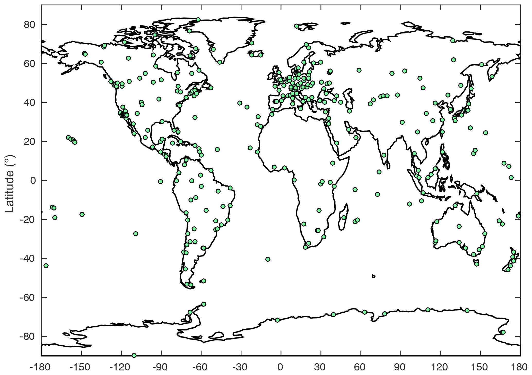
Figure 1Distribution of the GPS receiver stations used to derive the ungridded TEC used in the model evaluation in addition to the IGS GPS-TEC.
2.1.3 The disturbance storm time (Dst) index
The Dst index represents the axially symmetric disturbance magnetic field at the dipole equator on the Earth's surface. Major disturbances in Dst are negative, representing a decrease in the geomagnetic field. Therefore, days with a Dst value greater than −30 nT are assumed to be quite days and are included in the comparison of IRI-2016 with GPS-TECs. The 2 h Dst data are obtained from http://wdc.kugi.kyoto-u.ac.jp/dst_final/ (last access: 12 June 2020) for the 2 years.
2.2 Methodology
2.2.1 Numerical statistics: RMSE, bias, absolute mean error, normalized mean bias factor, normalized mean absolute error factor, and correlation
The comparison of TEC from the IRI-2016 model with GPS measurements is evaluated based on the RMSE, the bias, the MAE and its skill score (MAESS), the NMBF, the NMAEF, and the pattern correlation (R) between them for the selected years. The RMSE, which is the square root of the mean of all errors, indicates the deviation between simulated and observed data. It is given as
or
in terms of individual standard deviations (variances) of the simulations (σS), observations (σO), bias, and R between the two data sets. The bias discloses the mean difference between the simulated (IRI-TEC) and measured (GPS-TEC) data:
where Si and Oi are simulated and observed total electron content values, respectively, and n is the total number of data points for comparison. Although, the mean bias is a useful measure of the overall overestimation or underestimation by the model, and the RMSE includes this departure of the model from the observations and the scatter of the data around the mean, the RMSE is a problematic measure when there is an outlier in the data. As a result, the MAE is recommended as an alternative measure of model performance:
Furthermore, it is suitable to define model skill with respect to the reference model. To determine the model skill in connection with the reference model, the MAE for the reference model is first calculated with respect to the observations as follows:
where Sref represents the reference model simulations. The simplest consideration is to assume the reference model to be a model that can simulate only the mean observations accurately or a model that assumes the persistence of observations during a previous time into the following (future) time. Therefore, the skill score (MAESS) of the IRI-2016 model can be assessed as follows:
If the skill of IRI-2016 is not different from that of the reference model, MAESS will be approximately equal to zero. The more that MAESS diverges from zero towards larger positive values, the better the IRI-2016 model skill. Negative MAESS values imply that the IRI-2016 model skill is worse than that of the reference model.
The NMBF is computed from n pairs of modeled and observed TECs as
and
Similarly, the NMAEF is evaluated as
and
The NMBF and NMAEF are easier to interpret than the traditional comparison metrics. For example, a positive NMBF implies that the model overestimates the observations by a factor of NMBF+1; e.g., for NMBF=1.0, the model overestimates the observations by a factor of 2.0. Conversely, a negative NMBF indicates that the model underestimates the observations by a factor of 1−NMBF; for example, implies that the model underestimates the observations by a factor of 2.0 or 200 %. Thus, the NMBF metric reveals both the direction and magnitude of departure of the model prediction from observations. Similarly, the NMAEF can be used to infer the absolute gross error. For instance, if NMAEF=1.0, the absolute gross error is 1.0 times the mean observation when the model overestimates (i.e., MNBF>0, or ) or the absolute gross error is 1.0 times the model prediction when the model underestimates observations (i.e., NMBF<0, or ).
It is important to assess whether the model captures the diurnal and seasonal cycles of observed TEC in addition to the agreement in the TEC values between the model and the observations. The Pearson correlation (R) is usually applied to data sets that exhibit linearity and a Gaussian distribution to assess how the model performs in capturing the observed phase variation. Several studies have shown that TEC data for a limited number of days fulfill both of these conditions (Kumar et al., 2004; Zhang et al., 2005; Erdogan et al., 2017 and references therein). As a result, R is calculated for limited data that span a month to a maximum of a season in this study as follows:
R is also an indication of how much the spatial patterns in the IRI-2016 model match the IGS GPS observations (Murphy, 1998; Taylor, 2001; Daniel, 2006; Ochoa et al., 2014).
2.2.2 Categorical statistics: quantile probability of detection (QPOD), quantile categorical miss (QCM), and quantile critical success index (QCSI)
The categorical statistics employed in this study aim to evaluate the extent to which the simulation captures the distribution of the observed GPS-TEC above certain selected thresholds. As the IRI model is an empirical model based mainly on past observations, it is natural to expect that its performance at the extreme ends of the observed distribution may suffer from large inaccuracies. However, the extent of this discrepancy at the extreme ends of the observed TEC distribution is not assessed fully. Therefore, categorical statistics such as the QPOD, QCM, and QCSI are employed to evaluate the performance of the IRI-2016 model in simulating the whole range of observed distributions from extremely low to extremely high TECs. The QPOD defines part of the observations (O) above a selected percentile threshold (t) that is identified accurately by the simulation (S). It is given by
where H and M stand for hit and miss rates, respectively. H and M are given in terms of t, Oi, and Si as follows: and . A perfect detection signifies that the miss rate is zero implying that QPOD equals one. In contrast, a model with no skill has a zero hit rate, which suggests a QPOD value of zero. Therefore, QPOD attains a value of zero for no skill and one for a perfect score (Behrangi et al., 2011; AghaKouchak and Mehran, 2013).
The QCM may be defined as 1 − QPOD, and it varies from zero to one, with zero being a perfect score. The QCM can be given specifically in terms of the hit and miss rate as follows:
The QCSI combines various features of the QPOD and the quantile false alarm ratio (QFAR) in order to determine the total skill of the simulation relative to the observations as a function of H, M, and the false alarm rate (F):
The QCSI ranges from zero (no skill) to one (perfect skill) (Davis et al., 2009; AghaKouchak and Mehran, 2013). For example, a QCSI of 0.7 at a selected percentile threshold indicates that the simulation detects 70 % of the observed TEC above the selected percentile.
There are also other categorical metrics (e.g., QFAR) to assess model performance, but only the abovementioned metrics are used for brevity. Both of these numerical (continuous) and categorical statistics are used to assess the model skill in capturing the individual observations within the selected calendar months of March, June, September, and December in the case of the comparison between IRI-2016 and the GPS receiver station-level TEC and within seasons in the case of the comparison between the gridded IGS GPS-TEC and the IRI-2016 model during the solar minimum (2008) and maximum (2013; taken from window of solar maximum years 2012–2014).
3.1 Numerical statistics: RMSE, bias, MAE, MAESS, NMBF, NMAEF, and R
3.1.1 Comparison of the IRI-2016 simulation and station-level GPS-TEC observations
Figure 2 shows the R, RMSE, bias, MAE, and skill score (MAESS) determined from the comparison of IRI-2016 TEC simulations and station-level GPS-TEC observations for March, June, September, and December (see the legend) during the solar minimum in 2008 (Fig. 2a–e) and the solar maximum in 2013 (Fig. 2f–j). The correlation between the model and the individual measurements at global GPS stations, averaged within a given geomagnetic latitude band, ranges from 0.1 to 0.9 in 2008 (Fig. 2a) and from 0.3 to 0.91 in 2013 (Fig. 2f). The correlation between the measurements and the model is slightly better in 2013 than in 2008 along all geomagnetic latitude bands during all months. The RMSE in Fig. 2b is within the range of 3 to 15 TECU during 2008. The range of the RMSE in 2013 (Fig. 2g) is much higher (i.e., 4 to 25 TECU) than that in 2008. The RMSE generally decreases from the geomagnetic equator towards the poles with a few exceptions during both 2008 and 2013, which implies that the IRI-2016 model exhibits poor performance in capturing observed GPS-TEC over the tropics. This is also consistent with other metrics (see Fig. 2c–d for 2008 and Fig. 2h–i for 2013). Moreover, the difference between the model and GPS-TEC over the EIA crest regions is much higher than the for rest of the globe as noted from the high RMSE, bias, and MAE values in 2013. This holds also true in 2008 for the southern EIA crest region.

Figure 2The correlation, RMSE, bias, MAE, and MAESS determined from the comparison of TECs from IRI-2016 and the GPS receiver stations shown in Fig. 1 for 2008 (a–e) and 2013 (f–j). The statistical metrics are evaluated for the calendar months indicated by the legends.
The IRI-2016 TEC is biased high by up to 10 TECU over tropics with respect to GPS-TEC during 2008, whereas it is almost 2-fold higher in 2013 over the same region. A small negative bias is observed poleward of approximately 25∘ throughout the whole of 2008 and 2013 (Fig. 2c, h). However, a maximum positive bias in IRI-TEC with respect to GPS-TEC is observed over EIA crest regions (Fig. 2). This does not agree with a previous investigation by Kenpankho et al. (2011), who found that IRI-2007 underestimates GPS-TEC with a maximum difference of 15 TECU during daytime and a minimum variation of 5 TECU at night over an equatorial region in Thailand. However, the bias over mid and high latitudes is consistent with the findings from Grynyshyna-Poliuga et al. (2015), who showed that the TEC derived from the IRI-2012 model over a midlatitude station in Warsaw was generally biased low with respect to GPS-TEC. The maximum differences are about 10 TECU during daytime and 2 TECU at night. As noted by other authors (e.g., Akala et al., 2015, and references therein), the contribution from the plasmasphere above 2000 km in GPS-TEC might have contributed to the discrepancy over mid and high latitudes. For example, Akala et al. (2015) found that the contribution of the plasmasphere electron content to GPS-TEC is highest during the December solstice and lowest during the June solstice. This study also show a difference in the bias between the two seasons over the northern mid and high latitudes. Moreover, the authors noted that the plasmaspheric TEC contribution to GPS-TEC varies with respect to solar activity. The discrepancy between the IRI-2016 TEC simulations and GPS-TEC can not be fully attributed to the plasmasphere TEC as positive biases in IRI-2016 TEC are evidently dominant in the tropics. This positive bias with a maximum (up to 16.5 TECU) during the day and a minimum at night was also reported by Wan et al. (2017) at four stations in China covering the EIA crest region.
The skill score of the model with respect to the reference model that simulates mean TEC is assessed based on the MAE. The result shows that the IRI-2016 model performs better than the reference model at a few latitudes in the tropics (Fig. 2e, j) during both solar activity periods. It is also apparent that the model skill is worse than the reference climatological model during December (June) in the Southern (Northern) Hemisphere compared with the rest of the months for the low (high) solar activity year 2008 (2013) with slightly worst skill observed in 2013. The moderate skill in the tropics in general and the slightly better model skill during the low solar activity period than during the high solar activity period are in agreement with a previous study by Venkatesh et al. (2014), who conducted a comparison of GPS-TEC with the IRI-2012 modeled TEC over the Brazilian region during the period from 2010 to 2013 and found weak performance by the IRI model during a solar maximum.
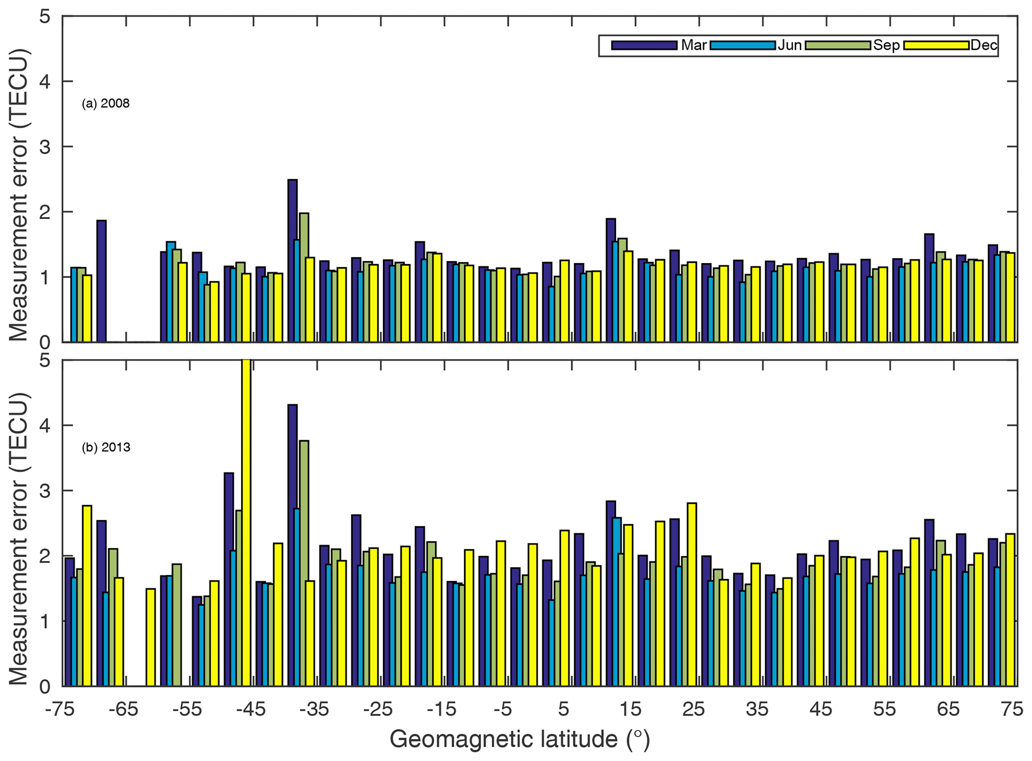
Figure 4Latitudinally averaged measurement errors during the calendar months shown in the legend for the two solar activity periods.
Li et al. (2016) determined a low bias in the nighttime modeled TEC during the solar minimum (2009) and the solar maximum (2013), and good (poor) agreement between periodic components of IRI-TEC in the low (high) solar activity year 2009 (2013). Moreover, the IRI-2016 model was investigated with respect to its performance over four stations in Ethiopia within the equatorial latitudes by Mengistu et al. (2018). The authors revealed better performance during solar minimum (2008) activity years than solar medium (2011) activity years. Other studies with a focus on high latitudes have shown a similar weakness in the IRI model. For example, IRI is also shown to significantly underestimate the magnitude of solar cycle variations in TEC and underestimate monthly median TEC at high solar activity by as much as 15 TECU (Themens and Jayachandran, 2016); these underestimations are greatest during the equinoxes and are significant during summer periods, and they are lowest during winter. These asymmetries, based on traditional metrics, suggest that IRI-2016 does not sufficiently capture enhanced TEC during the summer of each hemisphere when the sun is overhead at time of maximum solar activity. However, it is also important to note the difference in background TEC values during these seasons and the two low and high solar activity periods when using traditional model evaluation metrics. As noted in Sect. 1, the use of alternative metrics such as the NMBF and NMAEF to evaluate model skill may limit the problem that arises due to the difference in background TEC values.
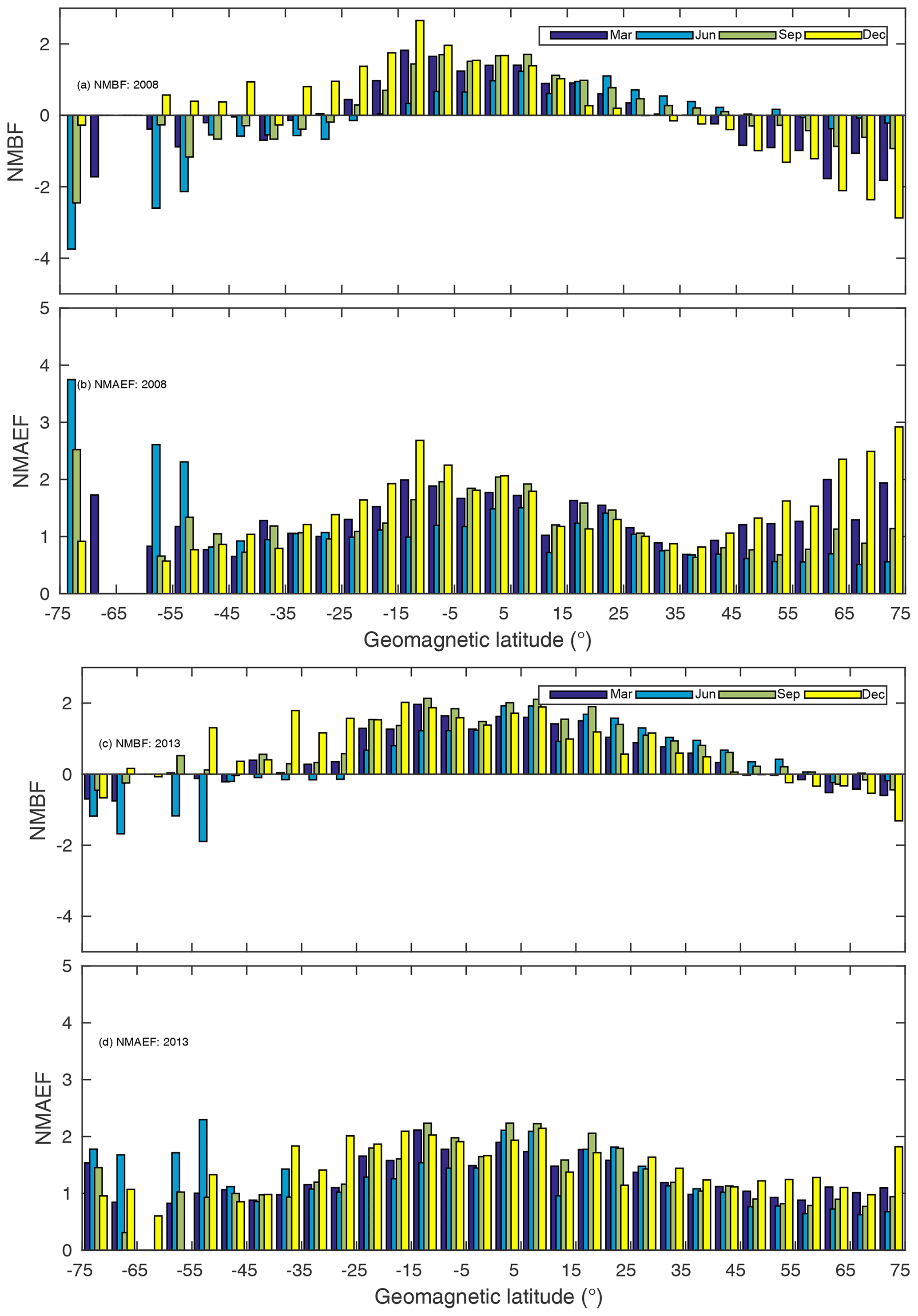
Figure 3a and c show that the IRI-2016 model overestimates the observations by up to a maximum factor of 3 in the tropics during the low (high) solar activity year 2008 (2013). Unlike the traditional metrics, this metric does not clearly show that the model performance is worse during the solar maximum than during the solar minimum over the tropics, as the difference in the NMBF between 2008 and 2013 is small. However, the model underestimates the observations over the high geomagnetic latitude region by up to a maximum factor of 4.5 in 2008 compared with a maximum factor of 3 in 2013 (Fig. 3b, d). Likewise, the NMAEF reveals that the model performance is relatively better in 2008 than in 2013.
The significance of the departure of the modeled TECs from observations can also be appreciated in the context of GPS observation errors. Figure 4 shows the total measurement errors in TEC from GPS receiver stations which is averaged over selected geomagnetic latitude bands for June, March, September, and December during 2008 and 2013. The maximum error in observed TEC in 2008 (Fig. 4a) is about 2.5 TECU, whereas it is about 5 TECU in 2013. These figures are far lower than the observed MAE or RMSE in Fig. 2b and d during 2008 and in Fig. 2f and h during 2013. Therefore, the overestimation or underestimation of observed TEC by IRI-2016 can be partially attributed to the discrepancy associated with the GPS measurement errors, albeit by a small fraction (up to an average of 2.5 and 4 TECU in 2008 and 2013, respectively).
3.1.2 Comparison of the IRI-2016 simulation and gridded IGS GPS-TEC observations at selected longitude sectors
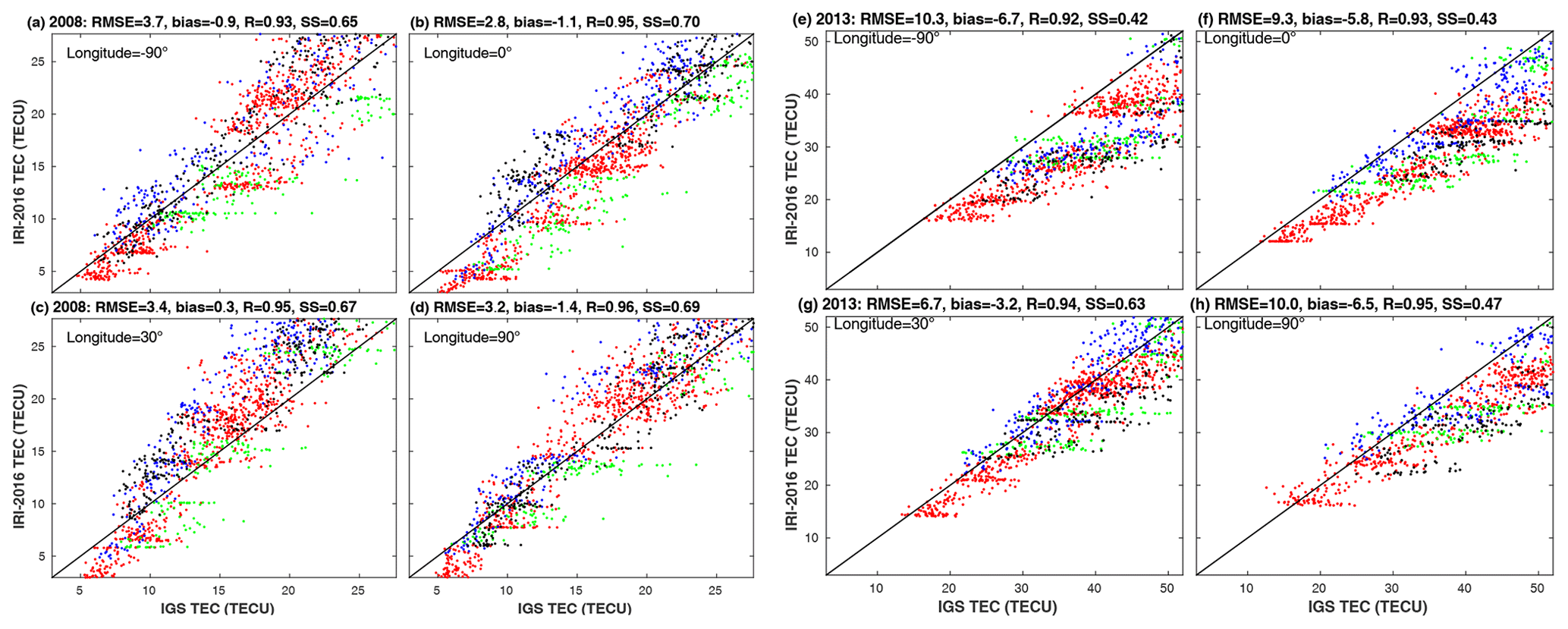
Figures 5 and 6 depict the comparison of IRI-2016 and GPS-TECs at four selected longitude sectors within the ±20∘ geomagnetic latitude band where the difference between the model and observations is high, as noted from Figs. 2 and 4. Figure 5 shows scatter plots of TECs from IRI-2016 versus IGS GPS at four selected longitudes during the morning hours of 00:00 to 10:00 LT (local time). The TEC is color coded to distinguish the different seasons (i.e., March equinox in green, June solstice in red, September equinox in blue, and December solstice in black). The TEC from IRI-2016 within the range from 10 to 30 TECU is biased high with respect to GPS-TEC during the September equinox (blue) at all longitudes, the December solstice (black) at longitudes of −90, 0, and 30∘, and the June solstice (red) at almost all longitudes in 2008. This also applies to the 2013 September equinox (blue) at all longitudes and the June solstice at a longitude of 30∘ for TEC values from 20 to 45 TECU (Fig. 5). In contrast, TEC from IRI-2016 is biased low against GPS-TEC during the March equinox (green points in Fig. 5) in 2008, whereas the bias is small in 2013. At the low tails of the observed and simulated TEC distribution during morning hours, the IRI-2016 model is biased low during all seasons in both the 2008 and 2013 solar activity periods.

Figure 5Scatter plots of TECs from IRI-2016 and GPS at selected longitudes for the solar minimum in 2008 (a–d) and the solar maximum in 2013 (e–h) for the morning hours' measurements and simulations. The data are colored according to season: March equinox (green), June solstice (red), September equinox (blue), and December solstice (black). The RMSE, bias, R, and skill score (SS) indicated at the top of each panel are calculated for the whole data set (all seasons and all observation times) within the ±20∘ geomagnetic latitude band.
Figure 6 shows the scatter plot for the observed and simulated TEC during afternoon hours from 12:00 to 22:00 LT. The IRI-2016 model is biased high against the observations during the September equinox (blue dots in Fig. 6) at all longitudes, the December solstice (black) at all longitudes, and the June solstice at longitudes of −90, 30, and 90∘ for observed TEC values between 10 and 25 TECU in 2008. During the March equinox, the model is biased low against GPS-TEC at longitudes of −90, 0, and 90∘. In contrast, the IRI-2016 model is biased low during all seasons in 2013 for the whole range of observed TEC during the afternoon hours. Close inspection of Figs. 5 and 6 reveals that the IRI-2016 model's performance in capturing afternoon observed TEC is weaker than that of its skill to simulate the morning (before noon) observed TEC during 2008. Moreover, this model weakness is amplified for observations during the solar maximum in 2013 for all seasons. The fact that the performance of the IRI-2016 model degrades with high solar activity has already been noted in Sect. 3.1.1, based on the RMSE, bias, MAE, and skill score.
Overall, the IRI-2016 TEC at the four selected longitudes is biased low (0.9 to 1.4 TECU) against GPS-TEC during 2008 with the exception of 30∘ longitude (see the panel headings of Figs. 5 and 6). In contrast, this bias increases to values ranging from 5.6 to 10.1 TECU during 2013. The skill score, based on the MAE and the reference model that only predicts the mean of the observations, varies from 0.65 to 0.70 in 2008 and from 0.43 to 0.63 in 2013. The performance of the model in capturing daytime TEC is better than for nighttime TEC, at least during the solar minima in 2008. Our findings regarding the longitudinal and seasonal differences in the performance of the IRI-2016 model during both the solar minimum in 2008 and the solar maximum in 2013 are consistent with the longitudinal and seasonal TEC variabilities (Scherliess et al., 2008; Fekadu et al., 2019). In particular, the model weakness during the afternoon hours might be linked to the wave number four pattern, which is created during the daytime hours at the equinox and the June solstice but is absent during the December solstice (Scherliess et al., 2008). Scherliess et al. (2008) showed enhancements in the TEC over Asia (near 100∘ E), America (near −90∘ E), and the Atlantic Ocean (the West Africa longitude sector near 0∘ E) in the afternoon hours during the equinox and the June solstice. The authors attributed the enhancements to the wave number four pattern. As the observed large RMSE, bias, and MAE within the tropics during both solar activity years are also from these seasons, it is highly probable that the weak model performance is due to these enhancements.
Moreover, the comparison between the model and the gridded GPS-TECs is extended to include the whole global region as given in Fig. 7 as a function of solar zenith angle (Fig. 7a–d) and magnetic local time (Fig. 7e–h). IRI-2016 is biased low at all solar zenith angles during the course of the day from sunrise to sunset in 2008 (Fig. 7a). However, the large biases in IRI-TECs are observed close to sunrise and sunset, whereas the lowest bias is observed near the noon solar zenith angle. In contrast, the highest negative bias in IRI-TEC in 2013 is noted at the noon solar zenith angle. Moreover, the negative bias decreases as a function of increasing solar zenith angle from the noon zenith angle towards sunset and sunrise in general with the exception of a couple of anomalies at 8 and 39∘ on the sunrise side (Fig. 7a, yellow bar). The RMSEs during both 2008 and 2013 peak shortly after the noon solar zenith angle is reached (Fig. 7b). The second peak in both bias and RMSE is observed around a solar zenith angle of 23∘ as the sun rises (Fig. 7a–b) in 2013. This peak in 2008 is only apparent in the RMSE (Fig. 7b). In addition to the dependence of the bias and RMSE on the solar zenith angle, the low bias in the IRI-2016 model ranges from values close to 0 to 2 TECU in 2008, whereas it varies from approximately 3 to 7 TECU in 2013. Similarly, the RMSE varies from approximately 0 to 5 TECU in 2008 and from 6.5 to 11 TECU in 2013, which is consistent with the differences noted between the two solar minimum and maximum periods in the analysis of TEC from individual GPS stations (see Fig. 2). Both the skill score (Fig. 7c) and the correlation (Fig. 7d) are consistent with the bias and RMSE as indicated by better model skill and a strong correlation at solar zenith angles with a minimum bias and RMSE than at solar zenith angles with a maximum negative bias and RMSE. It is also evident from the better skill score and high correlation that IRI-2016 performs better during the solar minimum than during the solar maximum period. The difference in the performance of the model during 2008 and 2013 is also apparently reflected in the bias, RMSE, skill score, and correlation as a function of magnetic local time (MLT; Fig. 7e–h). The negative bias in IRI-2016 decreases from midnight to noon and begins to increase thereafter during both 2008 and 2013 (Fig. 7e). The RMSE follows the same pattern until sunset (Fig. 7f). This pattern is similar to the percentage bias in foE from IRI-2012 compared with the foE obtained from the ionogram at the equatorial latitude station in Chumphon, Thailand (Wongcharoen et al., 2015). The skill score peaks from 12:00 to 14:00 MLT, whereas the correlation maximum is attained between 10:00 and 12:00 MLT (Fig. 7g–h). The poorest performances and lowest correlations are noted from approximately 3:00 to 6:00 MLT, i.e., post midnight (Fig. 7a–d). Therefore, the poor performance during this part of the diurnal cycle is indicative of the limitation of the semiempirical IRI-2016 model in terms characterizing some of the ionospheric parameters, specifically those with a similar diurnal pattern (e.g., foE, foF2, and NmF2), used in the model. Isolating the specific parameter or group of parameters that has a key role in influencing the model performance requires controlled sensitivity simulations over a range of parameter values. However, this is outside the scope of this study. The level of the strengths and weaknesses of IRI-2016 at the extreme parts of TEC distribution is further assessed in Sect. 3.2.1 and 3.2.2 using quantile-based categorical metrics.
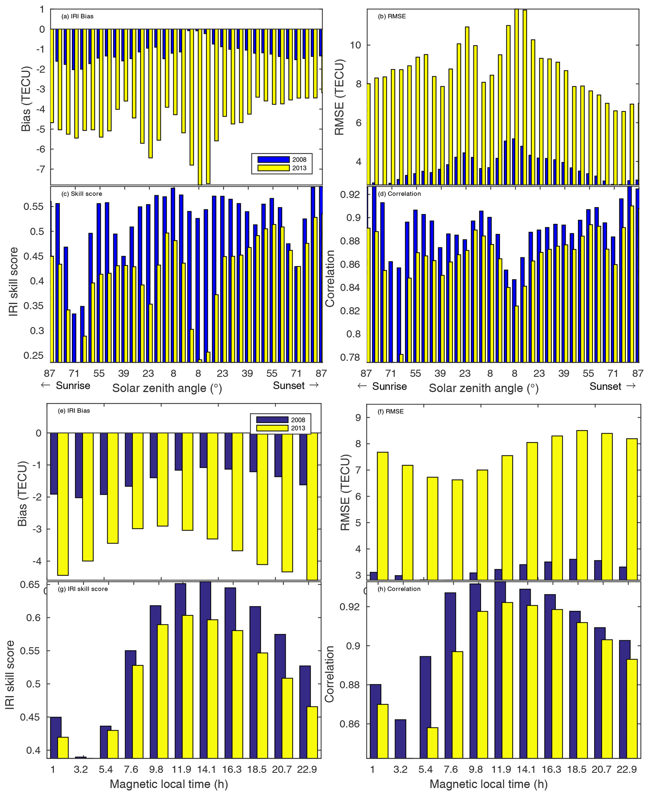
Figure 7The bias, RMSE, MAE-based skill score, and correlations between IRI-2016 and the gridded GPS-TECs as a function of daytime solar zenith angle (a–d) and magnetic local time (e–f) for 2008 (blue bar) and 2013 (yellow bar).
3.1.3 Comparison of the IRI-2016 simulation and IGS GPS-TEC observations on a seasonal basis
In previous sections, the comparisons were based on either individual data within a given calendar month (Sect. 3.1.1) or the whole year (Sect. 3.1.2). However, as we have noted in these sections, there is an indication that the model performance is a function of local time and seasons. Therefore, the calendar months are grouped into four seasons: the March equinox, the June solstice, the September equinox, and the December solstice. As noted in Sect. 3.1.1, traditional model evaluation metrics such as the RMSE, bias, and MAE are sensitive to differences in the background TEC values during the low (high) solar activity year 2008 (2013) as well as the magnitude of background TECs within different latitudinal regions. Therefore, the analysis in this section is based on the correlation, the MAE skill score, the NMBF, and the NMAEF.
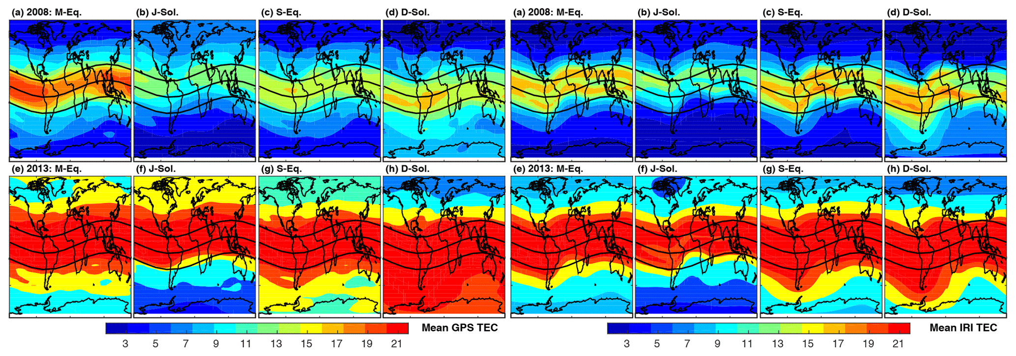
Figure 8The seasonal mean TEC obtained from the gridded IGS GPS-TEC (the eight left panels) and simulated by IRI-2016 (the eight right panels) for the March equinox (M-Eq), the June solstice (J-Sol), the September equinox (S-Eq), and the December solstice (D-Sol) during the solar minima year 2008 (top row) and the solar maxima year 2013 (bottom row).
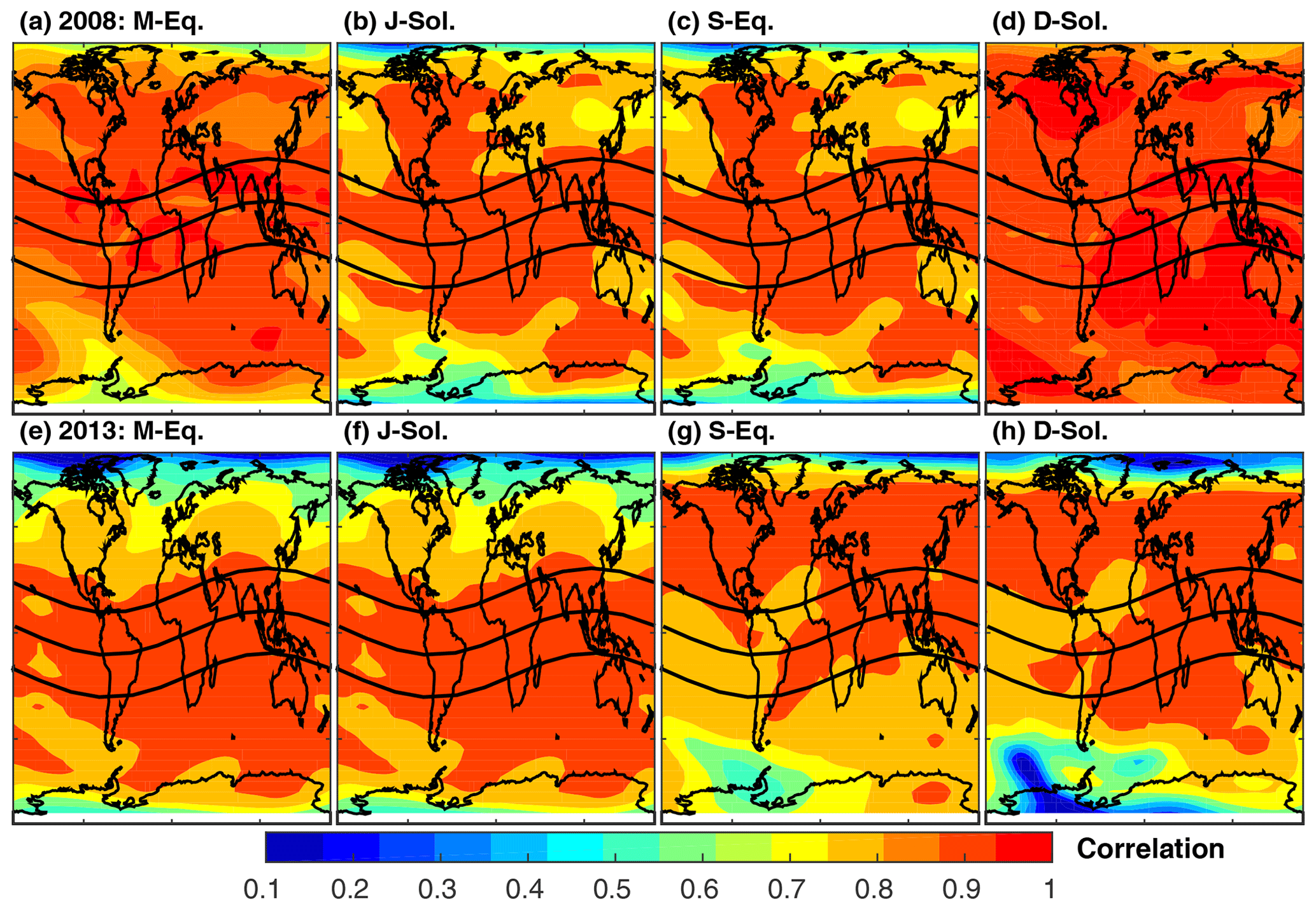
Figure 9Correlation between IRI-2016 and IGS GPS-TEC for the four seasons during 2008 (a–d) and 2013 (e–h).
In order to appreciate the NMBF and NMAEF values between the model and IGS GPS-TECs, the observed seasonal mean TECs and mean simulated TEC during the 2008 and 2013 seasons are given in Fig. 8. The maximum observed (Fig. 8a–d, left) and simulated (Fig. 8a–d, right) seasonal TEC during 2008 is confined to a geomagnetic latitude of ±20∘, as shown by the two solid outer lines on the map. In contrast, the maximum observed (Fig. 8e–h, left) and simulated (Fig. 8e–h, right) seasonal mean TEC in 2013 extend well into the high latitudes. In particular, the maximum seasonal mean covers nearly most of the Southern Hemisphere during the December solstice (Fig. 8h, left), whereas the extent of the peak seasonal mean TEC to high latitudes during the June solstice is minor. Moreover, the depletion of ionospheric TEC at the northern and southern polar latitudes during the December and June solstices, respectively, is worth noting during both low and high solar activity years. However, the low TEC latitude band covers wider areas during the June solstice than during the December solstice. The simulated seasonal mean TEC follows a similar pattern to the observed seasonal mean TEC (Fig. 8, right). In short, at the equinox, the TEC pattern is nearly symmetric about the geomagnetic equator, whereas large asymmetries are the major feature during the solstice. This morphology can be explained by considering the solar irradiance in the Southern and Northern hemispheres along with the direction of the neutral meridional wind during the different seasons. During the solstices, the neutral wind blows from the summer to the winter hemisphere, thereby raising the F-region ionization in the summer hemisphere and lowering it in the winter hemisphere. This wind effect and the asymmetry in the solar ionization and neutral composition in the two hemispheres are the main drivers of the observed asymmetries during the solstices, which are also captured by the IRI-2016 model (Scherliess et al., 2008; Mengistu Tsidu and Abraha, 2014; Fekadu et al., 2019).
In 2008 (the solar minimum period), the correlations are generally high in all seasons over most of the globe with the exception of the March and September equinoctial months and the June solstice over the southern Atlantic Ocean, the Pacific Ocean, and the polar regions, which had a low correlation between IRI-TEC and GPS-TEC (Fig. 9a–c). The December solstice in 2008 exhibits high correlations of 0.8 to 1.0 globally (Fig. 9d). The phase of TEC variation is well captured by the IRI-2016 model with some differences between seasons as revealed by the low correlation south of 50∘ S during the December solstice, south of 30∘ S during the September equinox, and north of 30∘ N during the June solstice and the March equinox in 2013. This confirms that relative to the correlation between IRI-TEC and GPS-TEC in 2008, there is a decrease in the correlation over these regions.
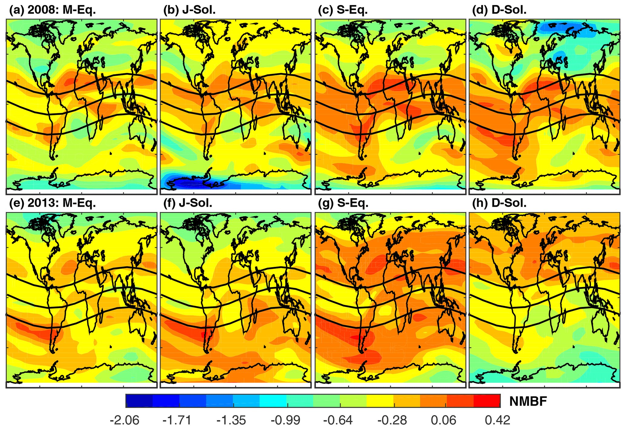
Figure 10The same as Fig. 9 but for NMBF.
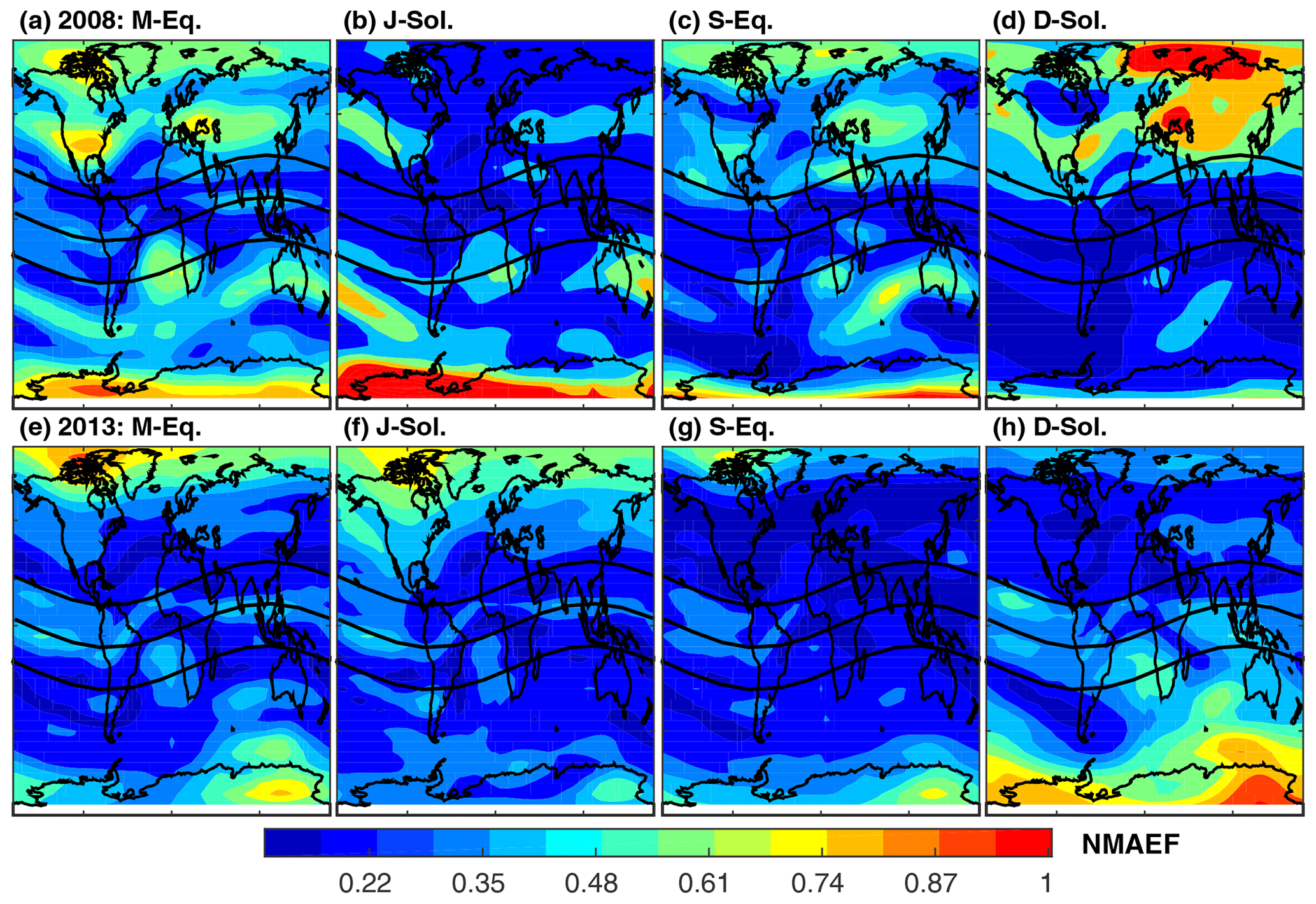
Figure 11The same as Fig. 9 but for NMAEF.
Generally, the NMBF implies that the IRI-2016 overestimates the observed TEC by a maximum factor of 1.4 within the ±20∘ geomagnetic latitude band in 2008 (Fig. 9). Moreover, the model overestimates the observations by almost the same factor over southern high latitudes during the September equinox and the December solstice. The model underestimates observed TEC over the rest of the globe by up to a factor of 2 on average (Fig. 10a–d). However, there are isolated pockets of areas over the northern polar region along the African longitude and the southern polar region along the American longitude sectors where the model underestimates observed TEC by a factor of 3 or 300 % (Fig. 10a–d) during the December and June solstices, respectively. In contrast, the model generally underestimates the observed TEC during all seasons in 2013 with the exception of an overestimation at a few localized pocket areas poleward of ±20∘. The TEC over the northern and southern polar regions during the June and December solstices have been underestimated by approximately a factor of 1.7 and 2, respectively. Figure 11 shows the NMAEF, which should be interpreted in conjunction with the NMBF. The overestimation within the ±20∘ geomagnetic latitude band during the solar minimum (2008) period in Fig. 10a–d occurred in conjunction with a NMAEF of approximately 0.2 or less which implies that the model overestimates TEC over these regions by maximum TEC values of 0.2 times the mean TEC in Fig. 8a–d (left panels). This means that the model has a high bias of roughly 2.6 to 4.2 TECU during the March equinox, 2 to 2.6 TECU during the June solstice, 2 to 2.8 TECU during the September equinox, and 2.8 to 3.4 TECU during the December solstice. Similarly, the NMAEF over the polar regions during all seasons in 2008 ranges from 0.6 to 1, which, in conjunction with the NMBF, implies that the model underestimates the observations by a factor of 0.6 to 1 times the simulated TEC in Fig. 8a–d (right panels) during the seasons (Fig. 11). This corresponds to approximately 1.8 to 3 TECU over the regions. The NMAEF within the ±20∘ geomagnetic latitude band in 2013 is also about 0.2 (Fig. 11e–h), implying an insignificant difference in the model performance between the low (2008) and high (2013) solar activity periods. The notable differences in the model performance between the two solar activity periods are over polar latitudes. The model performance during the solar minimum year (2008) with respect to the gridded IGS GPS-TEC is consistent with its performance with respect to TEC observations at individual GPS receiver stations. However, there is a notable difference between the model skill relative to IGS GPS-TEC and station-level TEC in 2013 over the ±20∘ geomagnetic latitude band, as revealed by the difference in the sign of the bias, whereas there is consistency between the two relative model skills over mid and high latitudes.
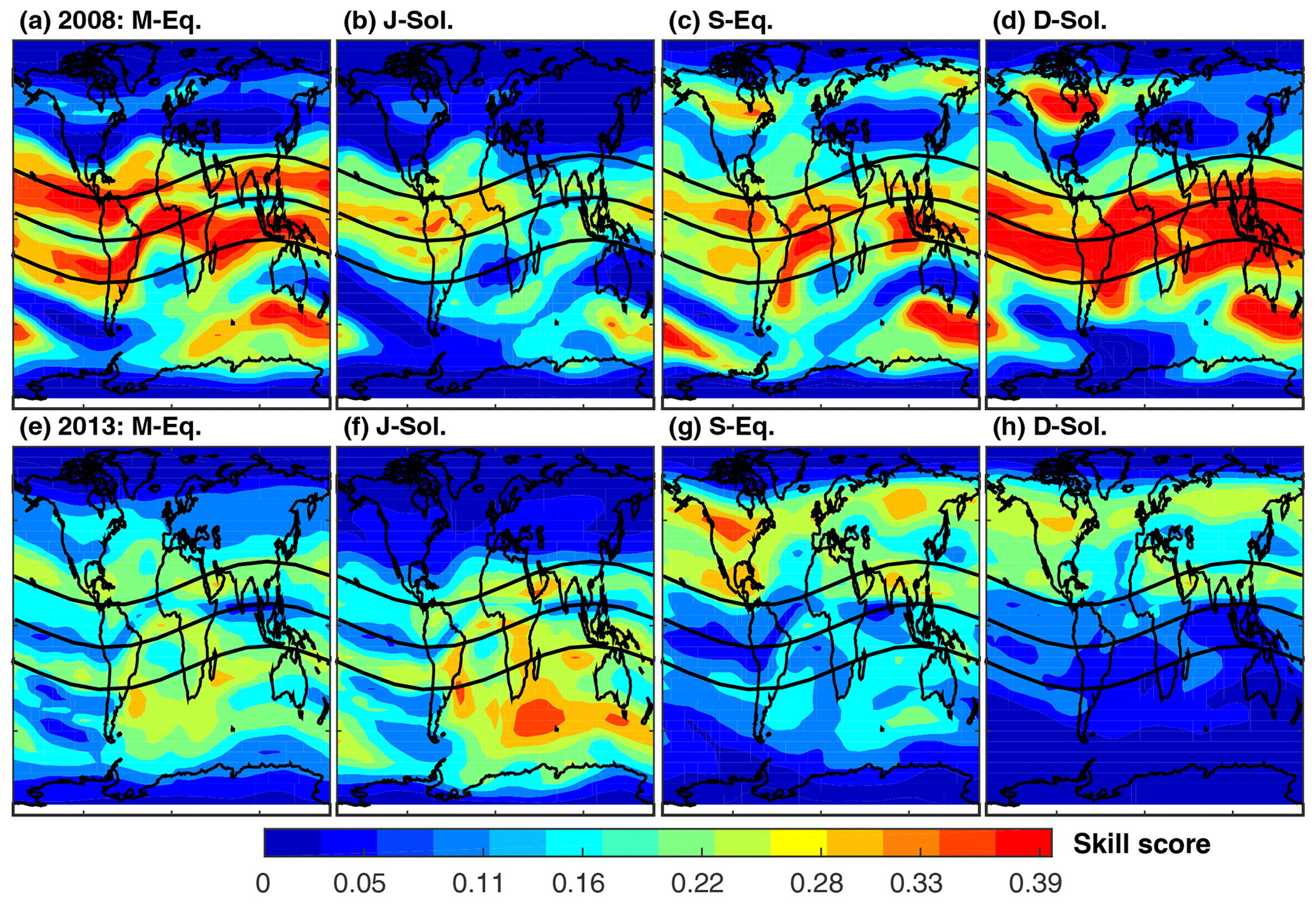
Figure 12The same as Fig. 9 but for the skill score.
Figure 12 shows the model skill score for the March equinox, the June solstice, the September equinox, and the December solstice during 2008 (Fig. 12a–d) and 2013 (Fig. 12e–h). In 2008 (the solar minimum period), the skill score of IRI-2016 was as high as 0.39 over large areas of the mid and tropical latitudes, which suggests that the IRI-2016 model is better than the climatological reference model and can capture TEC variability beyond the seasonal mean. Comparatively, the IRI-2016 model skill slightly weakened in 2013. As a result, IRI-2016 is better than just providing the seasonal mean TEC over ±20∘ geomagnetic latitudes and Southern Hemisphere midlatitudes during the March equinox and the June solstice. The model skill is also better than the reference model over regions between the geomagnetic equator and the northern midlatitudes during the September equinox and the December solstice. However, the model skill over the rest of the globe, in particular the polar regions, is no different from the reference climatological model. This is consistent with the conclusions drawn when the model is evaluated against TEC from GPS receiver stations in Sect. 3.1.1.
3.2 Categorical statistics: QPOD, QCM, and QCSI
3.2.1 Categorical comparison of the IRI-2016 simulation and GPS station-level TEC observations
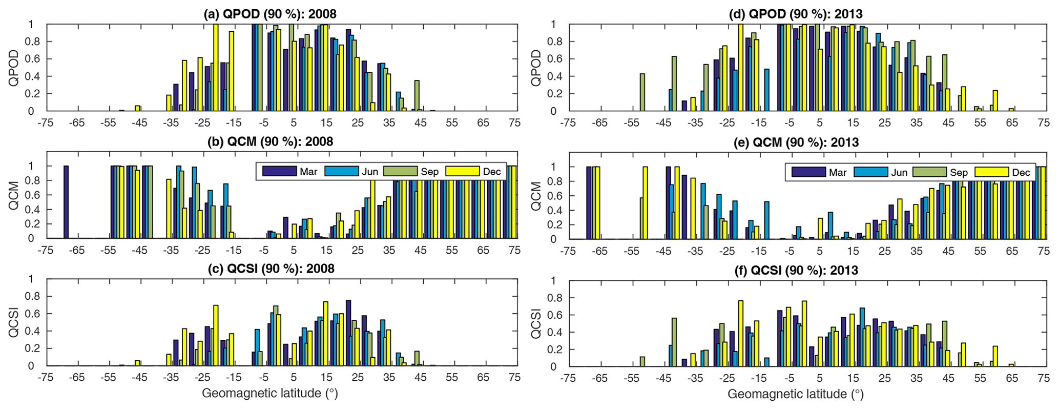
Figure 13 shows the QPOD, QCM, and QCSI for TEC values exceeding the 90th percentiles for the low (high) solar activity year 2008 (2013). The notable feature in Fig. 13 is the increase in the QPOD within the ±20∘ geomagnetic latitude band in 2013 (Fig. 13d) compared with 2008 (Fig. 13a). Consistent with this, the QCM shows values as high as one in mid and high geomagnetic latitudes and low values in the low-latitude regions (Fig. 13b, e). In contrast, there is a slight decrease in the QCSI in 2013 (Fig. 13f) compared with 2008 (Fig. 13c) during most of the seasons over northern geomagnetic latitudes. Near the geomagnetic equator and the Southern Hemisphere, the model skill in 2013 is slightly better than that during 2008. The difference in the pattern between the QPOD and QCSI is attributed to the increase in the false alarm rate at the high percentile threshold. This false model skill has been removed in the QCSI as opposed to the QPOD which shows high model skill. Therefore, we noticed here that the IRI-2016 model generally has better agreement with GPS during the solar minima in 2008 than during the solar maxima in 2013 at the extreme margins of the TEC distribution.
3.2.2 Categorical comparison of the IRI-2016 simulation and GPS-TEC observations on a seasonal basis
As noted in Sect. 3.1.2 from the scatter plots, most of the deviations from observations arise at the upper and lower ends of the TEC distribution. Therefore, efforts have been made to understand these discrepancies. For instance, Venkata Ratnam et al. (2017) included the relative TEC deviation index, monthly variations in the grand mean of ionospheric TEC, TEC intensity, and the upper and lower quartiles in their comparison of GPS-TEC with TECs predicted by IRI-2007 and IRI-2012. Although the inclusion of upper and lower quartiles is a step in the right direction with respect to understanding the discrepancy in these parts of the distribution, many of the observed differences lie in the extreme ends within the quartiles. Therefore, the application of quantile categorical statistics is necessary for more insight into the problem. Thus, the QPOD, the QCSI, and the QCM are employed in this section to assess the performance of IRI-2016 against GPS-TEC observations. The categorical metrics for the four seasons (the March equinox, the June solstice, the September equinox, and the December solstice) are given in Figs. 14 and 16 for 2008 and 2013.
Figure 14 depicts the QPOD for the March equinox (Fig. 14a–d), the June solstice (Fig. 14e–h), the September equinox (Fig. 14i–l), and the December solstice (Fig. 14m–p) during 2008 (first group of columns) and 2013 (last group of columns) at the 10th, 25th, 75th, and 90th percentiles. During 2008 (the March equinox season, left panels), the IRI-2016 model correctly identified over 80 % of the GPS-TEC exceeding the 10th percentile over broader areas along the geomagnetic equator and at isolated regions south of Australia (Fig. 14a). This figure remained the same at the 25th percentile (Fig. 14b). However, the QPOD increased to values exceeding 60 % over the rest of the tropics and midlatitudes. IRI-2016 captures more than 85 % of the observed TEC exceeding the 75th and 90th percentiles over the EIA crest region and exhibits a steady drop (to less than 20 %) in skill over the rest of the globe. Specifically, the change in the QPOD along the geomagnetic equator from values exceeding 80 % at the 10th percentile to values of less than 20 % at the 75th percentile is significant. The detection skill of the IRI model continued to decrease as the threshold increased from the 75th to the 90th percentile (Fig. 14c–d, left panels). As much of the nighttime and daytime TECs constitute low and high extremes in the climatology of TEC, it is consistent with previous understanding to observe a decline in model skill over the magnetic equator as the percentile threshold increases during 2008. Conversely, the performance of the model during the June solstice in identifying the lower ends of TEC distribution (values higher than the 10th percentile) greatly declined with a score of 60 %–80 % over the geomagnetic equator (Fig. 14e, left). However, at the 25th percentile (Fig. 14f, left), the QPOD increased over the magnetic equator and the northern Atlantic region to a value of 80 %–100 %. The QPOD at the 75th and 90th percentiles (Fig. 14g–h, left) decreased significantly over the magnetic equator as well as over the northern mid and high latitudes. In contrast to the March equinox, there is improvement in the model skill over the EIA crest region at these thresholds. The skill of the model remained poor at all thresholds over the southern polar regions during the June solstice (Fig. 14e–h, left). The performance of the model during the September equinox is shown in Fig. 14i–l. At the 10th percentile (Fig. 14i, left), the QPOD exceeds 80 % over the geomagnetic equator and at high latitudes, whereas much of the northern mid and high latitudes as well as areas between the tip of South Africa and Australia exhibit poor model skill with a QPOD of less than 20 %. At the 25th percentile (Fig. 14j, left), there is a significant increase in the QPOD over much of the globe. However, at the 75th and 90th percentiles (Fig. 14k–l), a decrease in the QPOD over the northern mid latitudes, polar regions, and the geomagnetic equator is observed. In contrast, there is an increase in the model skill over EIA regions. During the December solstice of 2008 at the 10th and 25th percentiles (Fig. 14m–n, left), the QPOD is within the range of 60 %–100 % over geomagnetic equator and the southern mid and high latitudes, whereas the QPOD is within 20 %–40 % over most of the northern mid and high latitudes. On the other hand, at the 75th and 90th percentiles (Fig. 14o–p, left), the QPOD improves to a value exceeding 80 % over EIA crest regions, whereas it decreases over both the northern and southern mid and high latitudes. The changes over the southern mid and high latitudes during this season at the 75th and 90th percentiles appear to be a mirror reflection of the June solstice in the Northern Hemisphere. This similarity in model detection skill during the two solstices is also apparent at the lower ends of TEC distribution. Unlike the June solstice, the high skill score covered most of the Southern Hemisphere (see Fig. 14m, left).
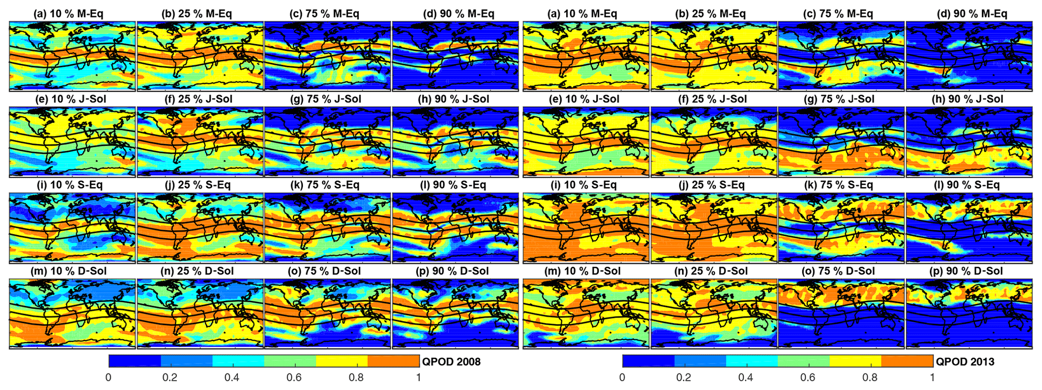
Figure 14The QPOD of the IRI-2016 model for the four seasons evaluated at the 10th, 25th, 75th, and 90th percentiles of the TEC distribution against GPS-TEC during the solar minima in 2008 (left panels) and the solar maxima in 2013 (right panels).
Table 1Statistical parameters of the QPOD for all seasonal variations of the solar minima in 2008 and the solar maxima in 2013.
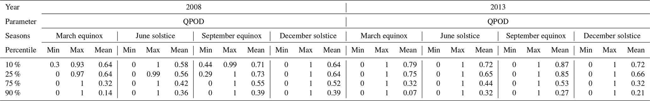
In 2013 during the solar maximum year, the QPOD characteristics are similar to that of 2008 for all the seasons but with a notable improvement at the lower ends of the distribution for the two equinoctial seasons (see Figs. 14a–b and i–j, right). In contrast to 2008, the model detection skill at the 75th and 90th percentiles weakened over the EIA crest regions. Instead, improved performance of the IRI-2016 model can be seen over most of the Southern and Northern hemispheres during the December and June solstices, respectively (Fig. 14g–h and o–p, right). Unlike the solstices, during the March and September equinoctial months, the performance at the 75th percentile is good over broader areas along EIA crest regions and is hemispherically symmetric (Fig. 14g, h, right). At the 90th percentile, the model performance is very bad over most parts of the globe during the March equinox and reasonably good over the northern midlatitudes during the September equinox (Fig. 14d, l, right). This suggests that the observed TEC distribution has slightly shifted towards higher values relative to 2008 as a whole, which is consistent with the high solar activity. This conclusion follows on from the fact that any improvement in model performance arises from the nature of the observed TEC distribution rather than the model itself, as the model configuration remained the same. This change in skill is also apparent within the same year from one season to another, as noted in the previous paragraph. Table 1 summarizes the changes in the QPOD with season and solar activity. The spatial minimum, maximum, and mean of QPOD at all percentile levels are indicated for the two solar activity periods. The minimum and maximum of the spatial mean QPOD at the 10th percentile occurred during the June solstice and the September equinox in 2008, respectively. However, the minimum and maximum of the spatial mean QPOD were observed during the December solstice and the September equinox in 2013, respectively. The lowest spatial mean QPOD at the 90th percentile was observed during the March equinox in 2008 and 2013, whereas the highest QPOD was seen during the September equinox and the September solstices in 2008 and during the June solstice in 2013.
Figure 15 shows the QCM at the 10th, 25th, 75th, and 90th percentiles for 2008 (left panels) and 2013 (right panels) for the four seasons, as in Fig. 14. As the QCM quantifies the TEC observed by GPS but missed by the IRI-2016 model, a perfect score is given by a QCM value of zero, whereas zero skill in the model is expressed by a QCM value of one. Therefore, the spatial patterns observed for the QPOD are expected to match that of the categorical miss, as shown in Fig. 15. The QCM is highest over high and polar latitudes during the June solstice and the March and September equinoctial seasons, whereas the tropics are generally characterized by low QCM values, which are consistent with QPOD features.
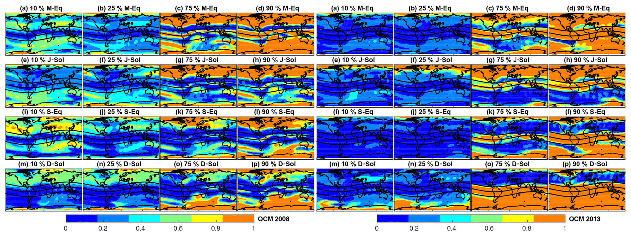
Figure 15The same as Fig. 14 but for QCM.
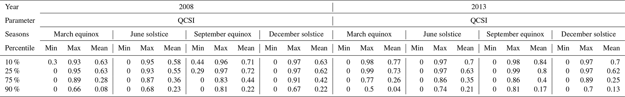
Figure 16 shows the QCSI at the four percentile levels during 2008 (left panels) and 2013 (right panels). The model performance, as assessed by the QCSI, remains the same as for the QPOD at the 10th and 25th percentiles (compare Figs. 14 and 15 with Fig. 16). However, the IRI-2016 performance, as revealed from the QCSI values, differs from that suggested by the QPOD at the 75th percentile during the December solstice and at the 90th percentiles during all seasons (Fig. 16o, d, h, l, p, left). This is due to the fact that the QCSI combines the QPOD and the QFAR features to describe the skill of the model in a more robust manner. However, the QCSI shows slightly higher model skill during 2013 at the lower ends of the distribution, as confirmed by the QCSI high value that ranged from 80 % to 100 % over most of the globe. Moreover, the skill of the IRI-2016 model at the high extreme tail of the TEC distribution during 2013 is relatively weaker than its performance in 2008 (Fig. 16d, h, l, p, right). Table 2 summarizes the globally averaged mean of the QCSI and its extremes during 2008 and 2013 for the four seasons. Clearly, the performance of IRI-2016 at the low extreme tail is better in 2013 than in 2008. The inverse is seen at the high extreme portion (90th percentile) of the TEC distribution, with lower QCSI values in 2013 than in 2008.
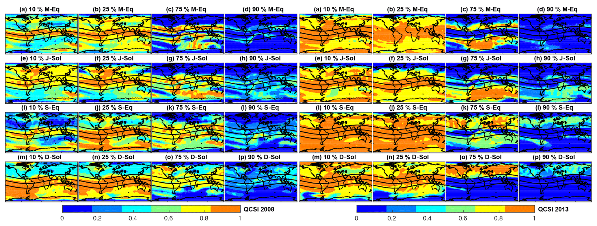
Figure 16The same as Fig. 14 but for QCSI.
Table 2Statistical parameters of the QCSI for all seasonal variations of the solar minima in 2008 and the solar maxima in 2013.
In this paper, the performance of the IRI-2016 model in simulating GPS-TEC is assessed by employing the RMSE, bias, MAE, NMBF, NMAEF, skill score, and correlation as well as categorical metrics such as the QPOD, QCM, and QCSI during two distinct solar activity periods. The IRI-2016 model simulations are based on the configuration that uses the latest developments.
The correlation between the model and individual measurements at GPS stations worldwide, averaged within a given geomagnetic latitude band, ranges from 0.1 to 0.9 in 2008 and from 0.3 to 0.91 in 2013. The RMSE generally decreases from the geomagnetic equator towards the poles with a few exceptions during both 2008 and 2013, implying that the IRI-2016 model exhibits poor performance in capturing observed TEC over the tropics. The IRI-2016 TEC is biased high by up to 10 TECU over the tropics with respect to TEC at the individual GPS receiver stations and averaged within the latitude bands during 2008. This figure is almost two-fold higher in 2013. However, the IRI-2016 bias over mid and high latitudes is negative with respect to the observed TECs at the GPS receivers sites, which is in agreement with some previous studies.
The skill score of the model with respect to the reference model that simulates mean TEC is assessed based on the MAE. The IRI-2016 model is found to perform worse than the reference model over high latitudes during the low (high) solar activity year 2008 (2013). Moreover, the model skill is worse than the reference climatological model during December (June) in the Southern (Northern) Hemisphere. The observed relatively good skill of the IRI-2016 model in the tropics and during low solar activity are in agreement with previous studies. Nevertheless, the traditional performance measures exaggerate the difference in the skill of the model during different solar activity periods as noted from minor differences in the NMBF and NMAEF during the two periods.
Investigation of the selected longitude sectors indicates that the IRI-2016 model is biased low at both the low and high tails of the TEC distribution, suggesting that IRI-2016 is capable of satisfactorily simulating the mean TEC globally. The longitudinal and seasonal variations in the performance of the IRI-2016 model can be explained in terms of the wave number four patterns as well as the difference in the solar insolation, neutral composition, and the direction of neutral meridional winds during these seasons. The dependence of the IRI-2016 performance on the solar zenith angle and magnetic local time reveals that the model requires further tuning of some of the ionospheric parameters used in the formulation of the bottom- and topside ionosphere. The extent of the IRI model strengths and weaknesses at the extreme portions of the observed TEC is assessed by categorical statistical metrics such as the QPOD, QCSI, and QCM using the 10th and 25th percentiles as lower margins and the 75th and 90th percentiles as upper margins of the TEC distribution for the two distinct solar activity periods. The performance of the IRI-2016 model based on individual GPS receiver measurements for the months of March, June, September, and December and gridded IGS GPS-TEC for the seasonal time series was evaluated using these thresholds. The model generally has reasonable skill at the low ends of TEC distribution over most of the globe. This skill weakens at the high ends of the TEC distribution over much of the globe except for EIA crest regions during both solar activity years. There is also hemispheric symmetry during the June and December solstices with poorer performance over the summer hemisphere at the high extremes of observed TEC. This feature is consistent with the high RMSE and low bias in the model during summer compared with winter. Similarly, the robust skill at the low ends of the observed TEC distribution can be attributed to the fact that low TECs which constitute the low portion of TEC distribution are mainly observed during nighttime, whereas those at the high ends of the distribution occur during daytime.
In summary, the IRI-2016 model, which itself is a climatological empirical model, has simulated a significant portion of the observed TEC over the tropics with better accuracy during both solar activity periods and the different seasons than a hypothetical model that only captures the seasonal mean TEC. The model performance at the extreme ends of the distribution is also remarkably good. In particular, the IRI model skill in detecting observed TEC over EIA crest regions at the extreme ends is robust despite the high RMSE. Therefore, this encouraging IRI-2016 model performance at the extreme ends of the observed TEC distribution suggests the importance of further work to improve the model so that it can be used for real-time operational forecasting.
Station-level GPS-TEC used in the study is available from the authors on request.
Conceptualization was by GMT and MMZ; investigation was by GMT and MMZ; data processing was done by GMT; the methodology was by GMT and MMZ; writing of the original draft was done by GMT and MMZ; writing, reviewing and editing were done by GMT.
The authors declare that they have no conflict of interest.
We are highly grateful to NASA for free access to the IRI-2016 model and GPS data. The authors would like to acknowledge the valuable input from Andrey Lyakhov and the anonymous reviewers. Moreover the second author extends his gratitude to Aksum University, Addis Ababa University, and the Botswana International University of Science and Technology (BIUST) for their financial support during second author's PhD study and research visit to BIUST.
This paper was edited by Dalia Buresova and reviewed by Andrey Lyakhov and two anonymous referees.
Acharya, R. and Majumdar, S.: Comparison of observed ionospheric vertical TEC over the sea in Indian region with IRI-2016 model, Adv. Space Res., 63, 1892–1904, 2019. a
AghaKouchak, A. and Mehran, A.: Extended contingency table: Performance metrics for satellite observations and climate model simulations, Water Resour. Res., 49, 7144–7149, https://doi.org/10.1002/wrcr.20498, 2013. a, b
AghaKouchak, A., Habib, E., and Bárdossy, A.: Modeling radar rainfall estimation uncertainties: Random error model, J. Hydrol. Eng., 15, 265–274, 2009. a
AghaKouchak, A., Nasrollahi, N., Li, J., Imam, B., and Sorooshian, S.: Geometrical characterization of precipitation patterns, J. Hydrometeorol., 12, 274–285, 2011a. a
Akala, A. O., Somoye, E. O., Adewale, A. O., Ojutalayo, E. W., Karia, S. P., Idolor, R. O., Okoh, D., and Doherty, P. H.: Comparison of GPS-TEC observations over Addis Ababa with IRI-2012 model predictions during 2010–2013, Adv. Space Res., 56, 1686–1698, 2015. a, b
Axelrad, P., Comp, C. J., and Macdoran, P. F: SNR-based multipath error correction for GPS differential phase, IEEE T. Aero. Elec. Sys., 32, 650–660, 1996. a
Bardhan, A., Malini, A., Sharma, D. K., and Rai, J.: Equinoctial asymmetry in low latitude ionosphere as observed by SROSS-C2 satellite, J. Atmos. Sol.-Terr. Phy., 117, 101–109, https://doi.org/10.1016/j.jastp.2014.06.003, 2014. a, b
Behrangi, A., Khakbaz, B., Jaw, T. C., AghaKouchak, A., Hsu, K., and Sorooshian, S.: Hydrologic evaluation of satellite precipitation products over a mid-size basin, J. Hydrol., 397, 225–237, 2011. a
Bilitza D.: International reference ionosphere: recent developments, Radio Sci., 21, 343–346, 2011. a
Bilitza, D.: International reference ionosphere 2000, Radio Sci., 36, 261–275, 2001. a
Bilitza, D., Rawer, K., Bossy, L., Kutiev, I., Oyama, K.-I., Leitinger, R., and Kazimirovsky, E.: International reference ionosphere 1990, Science Applications Research, Lanham, MD, USA, 1990. a, b, c, d
Bilitza, D., Rawer, K., Bossy, L., and Gulyaeva, T.: International reference ionosphere-past, present, and future: I. Electron density, Adv. Space Res., 13, 3–13, 1993a. a
Bilitza, D., Rawer, K., Bossy, L., and Gulyaeva, T.: International reference ionosphere-past, present, and future: II. plasma temperatures, ion composition and ion-drift, Adv. Space Res., 13, 15–23, 1993b. a
Bilitza, D., McKinnell, L. A., Reinisch, B., and Fuller-Rowell, T.: The international reference ionosphere today and in the future, J. Geod., 85, 909–920, https://doi.org/10.1007/s00190-010-0427-x, 2011. a
Bilitza, D., Altadill, D., Zhang, Y., Mertens, C., Truhlik, V., Richards, P., McKinnell, L.-A., and Reinisch, B.: The International Reference Ionosphere 2012 – a model of international collaboration, Journal of Space Weather Space Climate, 4, A07, https://doi.org/10.1051/swsc/2014004, 2014. a, b
Bilitza, D., Altadill, D., Truhlik, V., Shubin, V., Galkin, I., Reinisch, B., and Huang, X.: International Reference Ionosphere 2016: From ionospheric climate to real-time weather predictions, J. Space Weather, 15, 418–429, 2017. a, b, c
Borghetti, A., Corsi, S., Nucci, C. A., Paolone, M., Peretto, L., and Tinarelli, R.: On the use of continuous-wavelet transform for fault location in distribution power systems, Int. J. Elec. Power, 28, 608–617, https://doi.org/10.1016/j.ijepes.2006.03.001, 2006. a
Bossler, J. D., Goad, C. C., and Bender, P. L.: Using the Global Positioning System (GPS) for geodetic positioning, B. Géod., 54, 553, https://doi.org/10.1007/BF02530713, 1980. a
Daniel, S. W.: Statistical Methods in the Atmospheric Sciences, 2nd Edn., International Geophysics Series, 91 pp., Elsevier, San Diego, USA, 2006. a
Davis, C. A., Brown, B. G., Bullock, R., and Halley-Gotway, J.: The method for object-based diagnostic evaluation (MODE) applied to numerical forecasts from the 2005 NSSL/SPC Spring Program, Weather Forecast., 24, 1252–1267, 2009. a
Dorigo, W. A., Scipal, K., Parinussa, R. M., Liu, Y. Y., Wagner, W., de Jeu, R. A. M., and Naeimi, V.: Error characterisation of global active and passive microwave soil moisture datasets, Hydrol. Earth Syst. Sci., 14, 2605–2616, https://doi.org/10.5194/hess-14-2605-2010, 2010. a
Entekhabi, D., Reichle, R. H., Koster, R. D., and Crow, W. T.: Performance metrics for soil moisture retrievals and application requirements, J. Hydrometeorol., 11, 832–840, 2010. a
Erdogan, E., Schmidt, M., Seitz, F., and Durmaz, M.: Near real-time estimation of ionosphere vertical total electron content from GNSS satellites using B-splines in a Kalman filter, Ann. Geophys., 35, 263–277, https://doi.org/10.5194/angeo-35-263-2017, 2017. a
Feleke, F. D., Mengistu Tsidu, G., and Abraha, G.: Climatology of quasi-two day oscillations from GPS-derived total electron content during 1999–2015, Ad. Space Res., 64, 1046–1064, https://doi.org/10.1016/j.asr.2019.05.048, 2019. a, b, c
Gebremichael, M.: Framework for satellite rainfall product evaluation, Geophysical Monograph Series, 265–275, https://doi.org/10.1029/2010GM000974, AGU-Wiley, Washington, D.C., 2010. a
Gilleland, E., Ahijevych, D., Brown, B. G., Casati, B., and Ebert, E. E.: Intercomparison of spatial forecast verification methods, J. Weather Forecast., 24, 1416–1430, 2009. a
Grynyshyna-Poliuga, O., Stanislawska, I., Pozoga, M., Tomasik, L., and Swiatek, A.: Comparison of TEC value from GNSS permanent station and IRI model, Adv. Space Res., 55, 1976–1980, https://doi.org/10.1016/j.asr.2014.11.029, 2015. a, b, c
Hajj, G. A., Kursinski, E. R., Romans, L. J., Bertiger, W. I., and Leroy, S. S.: A technical description of atmospheric sounding by GPS occulation, J. Atmos. Sol.-Terr. Phy., 64, 451–469, 2002. a
Hernández-Pajares, M., Juan, J. M., Sanz, J., Aragon-Angel, A., Gracia-Rigo, A., Salazer, D., and Escudero, M.: The ionosphere: effects, GPS modeling and the benefits for space geodetic techniques, J. Geod., 85, 887–907, https://doi.org/10.1007/s00190-011-0508-5, 2011. a
Hoffmann, P. and Jacobi, C.: Analysis of planetary waves seen in ionospheric total electron content (TEC) perturbations, Wiss. Mitteil. Inst. Meteorol. Univ. Leipzig, 37, 29–40, 2006. a
Kenpankho, P., Watthanasangmechai, K., Supnithi, P., Tsugawa, T., and Maruyama, T.: Comparison of GPS TEC measurements with IRI TEC prediction at the equatorial latitude station, Chumphon, Thailand, Earth Planets Space, 63, 365–370, 2011. a, b
Komjathy, A.: Global ionospheric total electron content mapping using the Global Positioning System, University of New Brunswick Fredericton, New Brunswick, Canada, 1997. a
Kouris, S. S. and Fotiadis, D. N.: Ionospheric variability: a comparative statistical study, Adv. Space Res., 29, 977–985, 2002. a
Kouris, S. S., Xenos, T. D., Polimeris, K. V., and Stergiou, D.: TEC and foF2 variations: preliminary results, Ann. Geophys., 47, 1325-1332, https://doi.org/10.4401/ag-3346, 2004. a
Kumar, K. S., Kumar, C. V. A., George, B., Renuka, G., and Venugopal, C.: Analysis of the fluctuations of the total electron content (TEC) measured at Goose Bay using tools of nonlinear methods, J. Geophys. Res., 109, A02308, https://doi.org/10.1029/2002JA009768, 2004. a
Kumar, S.: Performance of IRI-2012 model during a deep solar minimum and a maximum year over global equatorial regions, J. Geophys. Res.-Space, 121, 5664–5674, https://doi.org/10.1002/2015JA022269, 2016. a
Kumar, S., Leong, E. T., Gulam, S. R., Samson, C. M. S., and Siingh, D.: Validation of the IRI-2012 model with GPS-based ground observation over a low-latitude Singapore station study, Earth Planets Space, 66, 1–17, 2014. a
Li, S., Li, L., and Peng, J.: Variability of ionospheric TEC and the performance of the IRI-2012 model at the BJFS station, China, Acta Geophys., 64, 1970–1987, https://doi.org/10.1515/acgeo-2016-0075, 2016. a
Liu, H., Wang, W., Richmond, A. D., and Roble, R. G.: Ionospheric variability due to planetary waves and tides for solar minimum conditions, J. Geophys. Res., 115, A00G01, https://doi.org/10.1029/2009JA015188, 2010. a
Liu, Z., Fang, H., Weng, L., Wang, S., Niu, J., and Meng, X.: A comparison of ionosonde measured foF2 and IRI-2016 predictions over China, Adv. Space Res., 63, 1926–1936, 2019. a
Lühr, H., Häusler, K., and Stolle, C.: Longitudinal variation of F region electron density and thermospheric zonal wind caused by atmospheric tides, Geophys. Res. Lett., 34, L16102, https://doi.org/10.1029/2007GL030639, 2007. a
Melbourne, W. G., Davis, E. S., Duncan, C. B., Hajj, G. A., Hardy, K. R., Kursinski, E. R., Meehan, T. K., Young, L. E., and Yunck, T. P.: The application of spaceborne GPS to atmospheric limb sounding and global change monitoring, National Aeronautics and Space Administration, Jet Propulsion Laboratory, California Institute of Technology National Technical Information Service, NASA, Pasadena, California, 1994. a
Mengistu, E., Damtie, B., Moldwin, M. B., and Nigussie, M.: Comparison of GPS-TEC measurements with NeQuick2 and IRI model predictions in the low latitude East African region during varying solar activity period (1998 and 2008–2015), Adv. Space Res., 61, 1456–1475, https://doi.org/10.1016/j.asr.2018.01.009, 2018. a, b
Mengistu Tsidu, G. and Abraha, G. F.: Moderate geomagnetic storms of January 22–25, 2012 and their influences on the wave components in ionosphere and upper stratosphere-mesosphere regions, Adv. Space Res., 54, 1793–1812, 2014. a, b, c, d
Mengistu Tsidu, G., Kidanu, G., and Abraha, G. F.: Tomographic Reconstruction of Ionospheric Electron Density Using Altitude-Dependent Regularization Strength over the Eastern Africa Longitude Sector, in: Ionospheric Space Weather, edited by: Fuller-Rowell, T., Yizengaw, E., Doherty, P. H., and Basu, S., https://doi.org/10.1002/9781118929216.ch11, AGU-Wiley, Washington, D.C., 2016. a
Morgan-Owen, G. J. and Johnston, G. T.: Differential GPS positioning, Electronics and Communication Engineering Journal (IET), 7, 11–21, 1995. a
Mosert, M., Gende, M., Brunini, C., Ezquer, R., and Altadill, D.: Comparisons of IRI TEC predictions with GPS and digisonde measurements at Ebro, Adv. Space Res., 39, 841–847, 2007. a
Mukherjee, S., Shivalika, S., Purohit, P. K., and Gwal, A. K.: Seasonal variation of total electron content at crest of equatorial anomaly station during low solar activity conditions, Adv. Space Res., 46, 291–295, https://doi.org/10.1016/j.asr.2010.03.024, 2010. a, b
Murphy, A. H.: Skill scores based on the mean square error and their relationships to the correlation coefficient, Mon. Weather Rev., 116, 2417–2424, 1998. a
Oberheide, J. and Gusev, O. A.: Observation of migrating and nonmigrating diurnal tides in the equatorial lower thermosphere, Geophys. Res. Lett., 29, 2167, https://doi.org/10.1029/2002GL016213, 2002. a
Ochoa, A., Pineda, L., Crespo, P., and Willems, P.: Evaluation of TRMM 3B42 precipitation estimates and WRF retrospective precipitation simulation over the Pacific–Andean region of Ecuador and Peru, Hydrol. Earth Syst. Sci., 18, 3179–3193, https://doi.org/10.5194/hess-18-3179-2014, 2014. a
Onohara, A. N., Batista, I. S., and Takahashi, H.: The ultra-fast Kelvin waves in the equatorial ionosphere: observations and modeling, Ann. Geophys., 31, 209–215, https://doi.org/10.5194/angeo-31-209-2013, 2013. a
Perna L., Pezzopane, M., Ezquer, R., Cabrera, M., and Baskaradas, J. A.: NmF2 trends at low and mid latitudes for the recent solar minima and comparison with IRI-2012 model, Adv. Space Res., 60, 363–374, https://doi.org/10.1016/j.asr.2016.09.025., 2017. a, b
Perna, L., Venkatesh, K., Pillat, V. G., Pezzopane, M., Fagundes, P. R., Ezquer, R. G., and Cabrera, M. A.: Bottom side profiles for two close stations at the southern crest of the EIA: Differences and comparison with IRI-2012 and NeQuick2 for low and high solar activity, Adv. Space Res., 61, 295–315, https://doi.org/10.1016/j.asr.2017.10.007, 2018. a, b
Praveen, G., Dashora, N., Sharma, S., and Pandey, R.: Characterization of low latitude GPS-TEC during very low solar activity phase, J. Atmos. Sol.-Terr. Phy., 72, 1309–1317, 2010. a
Rao, S. S., Monti, C., and Pandey, R.: Ionospheric variations over Chinese EIA region using foF2 and comparison with IRI-2016 model, Adv. Space Res., 62, 84–93, https://doi.org/10.1016/j.asr.2018.04.009, 2018. a, b, c
Rawer, K.: Synthesis of ionospheric electron density profiles with Epstein functions, Adv. Space Res., 8, 191–198, 1988. a
Rawer, K., Bilitza, D., and Ramakrishnan, S.: International reference ionosphere 78. Special Report, International Union of Radio Science (URSI), Brussels, Belgium, 1978. a
Saranya, P. L., Prasad, D. S. V. V. D., and Rama Rao, P. V. S.: Ionospheric vertical drifts over an Indian low latitude station and its comparison with IRI-2007 vertical drift model, Adv. Space Res., 54, 946–954, https://doi.org/10.1016/j.asr.2014.05.026, 2014. a, b
Scherliess, L., Thompson, D. C., and Schunk, R. W.: Longitudinal variability of low-latitude total electron content: Tidal influences, J. Geophys. Res., 113, A01311, https://doi.org/10.1029/2007JA012480, 2008. a, b, c, d
Schreiner, W. S., Sokolovskiy, S. V., Rocken, C., and Hunt, D. C.: Analysis and validation of GPS/MET radio occulation data in the ionosphere, Radio Sci., 34, 949–966, 1999. a
Sethi, N. K., Dabas, R. S., and Sarkar, S. K.: Validation of IRI-2007 against TEC observations during low solar activity over Indian sector, J. Atmos. Sol.-Terr. Phy., 73, 751–759, 2011. a, b
Sharma, D. K., Malini, A., and Ananna, B.: Variability of ionospheric parameters during solar minimum and maximum activity and assessment of IRI model, Adv. Space Res., 60, 435–443, https://doi.org/10.1016/j.asr.2016.11.027, 2017. a, b
Shubin, V. N.: Global median model of the F2-layer peak height based on ionospheric radio-occulation and ground-based Digisonde observations, Adv. Space Res., 56, 916–928, 2015. a
Shubin, V. N., Karpachev, A. T., and Tsybulya, K. G.: Global model of the F2 layer peak height for low solar activity based on GPS radio-occulation data, J. Atmos. Sol.-Terr. Phy., 104, 106–115, 2013. a
Takahashi, H., Lima, L. M., Wrasse, C. M., Abdu, M. A., Batista, I. S., Gobbi, D., Buriti, R. A., and Batista, P. P.: Evidence on 2–4 day oscillations of the equatorial ionosphere hF and mesospheric air glow emissions, Geophys. Res. Lett., 32, L12102, https://doi.org/10.1029/2004GL022318, 2005. a
Takahashi, H., Wrasse, C. M., Pancheva, D., Abdu, M. A., Batista, I. S., Lima, L. M., Batista, P. P., Clemesha, B. R., and Shiokawa, K.: Signatures of 3–6 day planetary waves in the equatorial mesosphere and ionosphere, Ann. Geophys., 24, 3343–3350, https://doi.org/10.5194/angeo-24-3343-2006, 2006. a
Takahashi, H., Wrasse, C. M., Fechine, J., Pancheva, D., Abdu, M. A., Batista, I. S., Lima, L. M., Batista, P. P., Clemesha, B. R., Schuch, N. J., Shiokawa, K., Gobbi, D., Mlynczak, M. G., and Russel, J. M.: Signatures of ultra-fast Kelvin waves in the equatorial middle atmosphere and ionosphere, Geophys. Res. Lett., 34, L11108, https://doi.org/10.1029/2007GL029612, 2007. a
Takahashi, H., Abdu, M. A., Wrasse, C. M., Fechine, J., Batista, I. S., Pancheva, D., Lima, L. M., Batista, P. P., Clemesha, B. R., Shiokawa, K., Gobbi, D., Mlynczak, M. G., and Russel, J. M.: Possible influence of ultra-fast Kelvin wave on the equatorial ionosphere evening uplifting, Earth Planets Space, 61, 455–462, 2009. a
Tariku, Y. A.: TEC prediction performance of IRI-2012 model during a very low and a high solar activity phase over equatorial regions, Uganda, J. Geophys. Res.-Space, 120, 5973–5982, 2015. a, b
Taylor, K. E.: Summarizing multiple aspects of model performance in a single diagram, J. Geophys. Res.-Atmos., 106, 7183–7192, 2001. a
Themens, D. R. and Jayachandran, P. T.: Solar activity variability in the IRI at high latitudes: Comparisons with GPS total electron content, J. Geophys. Res.-Space, 121, 3793–3807, 2016. a, b, c
Venkata Ratnam, D., Sivavaraprasad, G., and Devi, N. L.: Analysis of ionosphere variability over low-latitude GNSS stations during 24th solar maximum period, Adv. Space Res., 60, 419–434, 2017. a, b, c, d
Venkatesh, K., Fagundes, P. R., Seemala, G. K., de Jesus, R., de Abreu, A. J., and Pillat, V. G.: On the performance of the IRI-2012 and NeQuick2 models during the increasing phase of the unusual 24th solar cycle in the Brazilian equatorial and low-latitude sectors, J. Geophys. Res.-Space, 119, 5087–5105, https://doi.org/10.1002/2014JA019960, 2014. a
Wan, Q., Guanyi, M., Jinghua, L., Xiaolan, W., Jiangtao, F., Qi, L., and Weijun, L.: A comparison of GPS-TEC with IRI-TEC at low latitudes in China in 2006, Adv. Space Res., 60, 250–256, https://doi.org/10.1016/j.asr.2016.12.002, 2017. a
Wang, S., Huang, S., Fang, H., and Wang, Y.: Evaluation and correction of the IRI2016 topside ionospheric electron density model, Adv. Space Res., 58, 1229–1241, 2016. a
Wongcharoen, P., Kenpankho, P., Supnithi, P., Ishii, M., and Tsugawa, T.: Comparison of E layer critical frequency over the Thai station Chumphon with IRI, Adv. Space Res., 55, 2131–2138, 2015. a
Woo, K. T.: Optimum semicodeless carrier-phase tracking of L2, Navigation, 47, 82–99, https://doi.org/10.1002/j.2161-4296.2000.tb00204.x., 2000. a
Wu, Q., Solomon, S. C., Kuo, Y. H., Killeen, T. L., and Xu, J.: Spectral analysis of ionospheric electron density and mesospheric neutral wind diurnal nonmigrating tides observed by COSMIC and TIMED satellites, Geophys. Res. Lett., 36, L14102, https://doi.org/10.1029/2009GL038933, 2009. a
Yekoye, A., Kassa, T., and Nigussie, M.: Validation of IRI-2012 TEC model over Ethiopia during solar minimum (2009) and solar maximum (2013) phases, Adv. Space Res., 53, 1582–1594, https://doi.org/10.1016/j.asr.2014.02.017, 2014. a, b, c
Yu, S., Brian, E., Robin, D., Shao-Hang, C., and Stephen, E. S.: New unbiased symmetric metrics for evaluation of air quality models, Atmos. Sci. Lett., 7, 26–34, https://doi.org/10.1002/asl.125 2006. a
Zhang, H., Wang, J., Zhu, W.-Y., and Huang, C.: Gaussian random process and its application for detecting the ionospheric disturbances using GPS, Journal of Global Positioning Systems, 4, 76–81, 2005. a
Zhang, M.-L., Radicella, S. M., Shi, J.-K., Wang, X., and Wu, S.-Z.: Comparison among IRI, GPS-IGS and ionogram-derived total electron contents, Adv. Space Res., 37, 972–977, 2006. a