the Creative Commons Attribution 4.0 License.
the Creative Commons Attribution 4.0 License.
 | 18 Mar 2020
Ionosonde total electron content evaluation using International Global Navigation Satellite System Service data
Telmo dos Santos Klipp
Adriano Petry
Jonas Rodrigues de Souza
Eurico Rodrigues de Paula
Gabriel Sandim Falcão
Haroldo Fraga de Campos Velho
In this work, a period of 2 years (2016–2017) of ionospheric total electron content (ITEC) from ionosondes operating in Brazil is compared to the International GNSS (Global Navigation Satellite System) Service (IGS) vertical total electron content (vTEC) data. Sounding instruments from the National Institute for Space Research (INPE) provided the ionograms used, which were filtered based on confidence score (CS) and C-Level flag evaluation. Differences between vTEC from IGS maps and ionosonde TEC were accumulated in terms of root mean squared error (RMSE). As expected, we noticed that the ITEC values provided by ionosondes are systematically underestimated, which is attributed to a limitation in the electron density modeling for the ionogram topside that considers a fixed scale height, which makes density values decay too rapidly above ∼800 km, while IGS takes in account electron density from GNSS stations up to the satellite network orbits. The topside density profiles covering the plasmasphere were re-modeled using two different approaches: an optimization of the adapted α-Chapman exponential decay that includes a transition function between the F2 layer and plasmasphere and a corrected version of the NeQuick topside formulation. The electron density integration height was extended to 20 000 km to compute TEC. Chapman parameters for the F2 layer were extracted from each ionogram, and the plasmaspheric scale height was set to 10 000 km. A criterion to optimize the proportionality coefficient used to calculate the plasmaspheric basis density was introduced in this work. The NeQuick variable scale height was calculated using empirical parameters determined with data from Swarm satellites. The mean RMSE for the whole period using adapted α-Chapman optimization reached a minimum of 5.32 TECU, that is, 23 % lower than initial ITEC errors, while for the NeQuick topside formulation the error was reduced by 27 %.
- Article
(4403 KB) - Full-text XML
- BibTeX
- EndNote


The understanding of ionospheric behavior provides important information about the space weather. In addition, the electron content affects group and phase delays of radio waves passing through the ionosphere and impacts, among others, the Global Navigation Satellite System (GNSS). Different instruments are capable of evaluating electron density in the ionosphere, and validations among different sources of data can lead to interesting conclusions. While ionosonde instruments provide “ground truth” measures for the bottom side of the ionospheric profile and estimate the topside using an exponential decay function, ground GNSS stations receiving radio signals from orbiting satellites can provide large-scale details of the entire ionosphere structure and even plasmasphere (Huang and Reinisch, 2001; Reinisch and Huang, 2001; Jakowski, 2005; Reinisch and Galkin, 2011; Jin and Jin, 2011). The analysis proposed in this work is based on comparisons between total electron content (TEC) estimated using density profiles derived from ionograms and vertical total electron content (vTEC) from the International GNSS Service (IGS). While the IGS has its own intrinsic quality control through a ranking system (Hernández-Pajares et al., 2009), ionosonde data are evaluated by its auto-scaling system, and quality scores are assigned to each ionogram. The study was performed in the Brazilian region for a 2-year period (2016–2017), where ionosonde data from National Institute for Space Research (INPE) were available. Indeed, the plasmaspheric electron density has been considered using two different models: an adapted α-Chapman function (Jakowski, 2005) with a simple optimization and a corrected version of the NeQuick topside formulation (Pezzopane and Pignalberi, 2019).
1.1 IGS vTEC maps
IGS vTEC maps are considered to be a reliable ionospheric information product, which was achieved from integrating scientific community efforts (Hernández-Pajares et al., 2009). Such maps are generated by a combination of data from different research institutions within a method that is based on ranking different vTEC maps to compose the final product (Hernández-Pajares et al., 2009). The process begins with raw data from the GNSS ground network being acquired and sent to Ionospheric Associate Analysis Centers (IAACs) so the vTEC maps can be generated using the IONosphere map EXchange (IONEX) format (Schaer et al., 1998). To achieve a high level of quality, these vTEC maps are evaluated, and its ability to reproduce corresponding slant TEC (STEC) maps is checked. Next, a combination process takes place using a weighted mean of the available vTEC maps. The final step before making the maps available for access on the IGS server is a validation process. It compares the vTEC maps to an independent source: dual-frequency altimeters onboard the TOPEX, JASON, and ENVISAT satellites.
1.2 Ionosonde data
An ionosonde measures the returning echoes of pulse signals at a fixed location to estimate ionospheric characteristics, and the ionogram trace can be processed to result in a vertical electron density profile. The bottom side profile starts with measures at ∼90 km up to the peak of the F2 layer (foF2), around 350 km. The ionosphere topside profile, instead, is modeled using an exponential decay function. The integration of electron density in height produces an estimate for the TEC value.
Ionograms can be interpreted either manually by experts or automatically using software. The auto-scaling ionosonde data availability, rather than manual scaling, contributes to meeting practical applications (Jiang et al., 2015). Different systems were created and concentrated efforts have been applied to improve auto-scaling (Reinisch and Xueqin, 1983; Scotto and Pezzopane, 2002, 2007; Reinisch et al., 2005). Also, a standard archiving output (SAO) format was created by the initiative of the Ionospheric Informatics Working Group (IIWG) to store and disseminate auto-scaled data. Initially, SAO format considered only ionograms scaled by an automatic real-time ionogram scaler with true height (ARTIST); however, it evolved to hold scaled data from other sounder systems (Galkin, 2006).
Table 1Correspondent CS values for C-Level flag representation, adapted from Galkin et al. (2013).
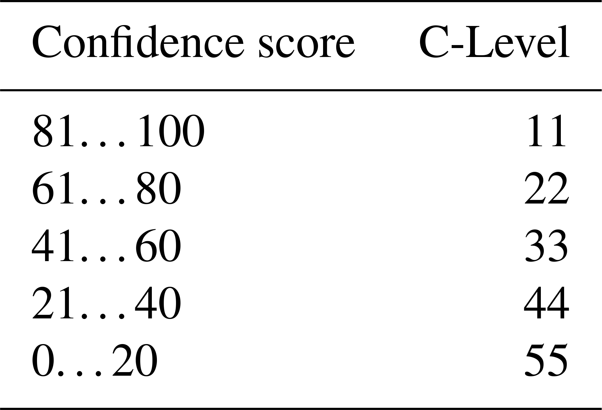
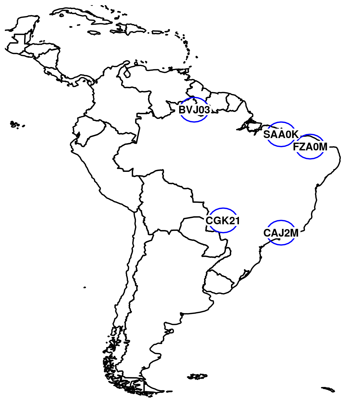
Figure 1Locations of available ionosonde data during 2016–2017.
Ionogram quality
Several attempts had been made to verify ionogram auto-scaling system quality (Reinisch et al., 2005; Enell et al., 2016; Pezzopane et al., 2017). Early comparisons between manual and automatic scaled ionospheric parameters revealed limitations in ARTIST system performance due to the absence of quality metrics (Gilbert and Smith, 1988). Recent versions of the ARTIST system improved quality-proof methods, enhancing their results (Bamford et al., 2008; Galkin and Reinisch, 2008) and facing problems related to auto-scaling (Pezzopane and Scotto, 2007; Stankov et al., 2012).
Ionosonde data scaled by ARTIST 5 have a quality metric called the confidence score (CS). Such a metric is based on quality criteria supported by concepts of ionogram interpretation and algorithms that specify the uncertainty and confidence of scaled results (Galkin et al., 2013). The CS metric includes quality checking solutions introduced by confidence calculation schemes developed since the late 1980s: the auto-scaling confidence level (ACL) quality flag, the two-digit confidence level (C-Level), and the QualScan quality control (McNamara, 2006; Galkin et al., 2013). The estimation of the confidence score occurs during ionogram processing. Ionogram interpretation criteria consider not only analysis of extracted trace shapes, but also ionospheric conditions to compute per-point-error reduction. The CS starts with a value of 100. If an interpretation criterion is found, its per-point-error value is subtracted from the CS. To be considered acceptable for further use, auto-scaling records need to reach a CS above a predefined threshold value, which is generally 40 (Galkin et al., 2013).
The SAO format version 4 does not have the CS on its specifications, but has the C-Level representation. The two digits' range goes from 11 (highest confidence) to 55 (lowest confidence). The CS produced by ARTIST 5 can be converted to C-Level representation using Table 1 (Galkin et al., 2013).
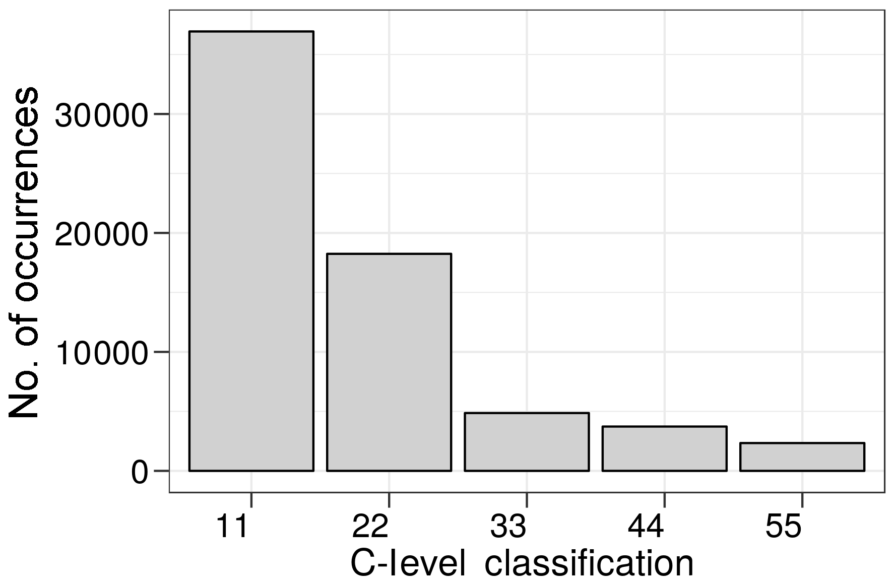
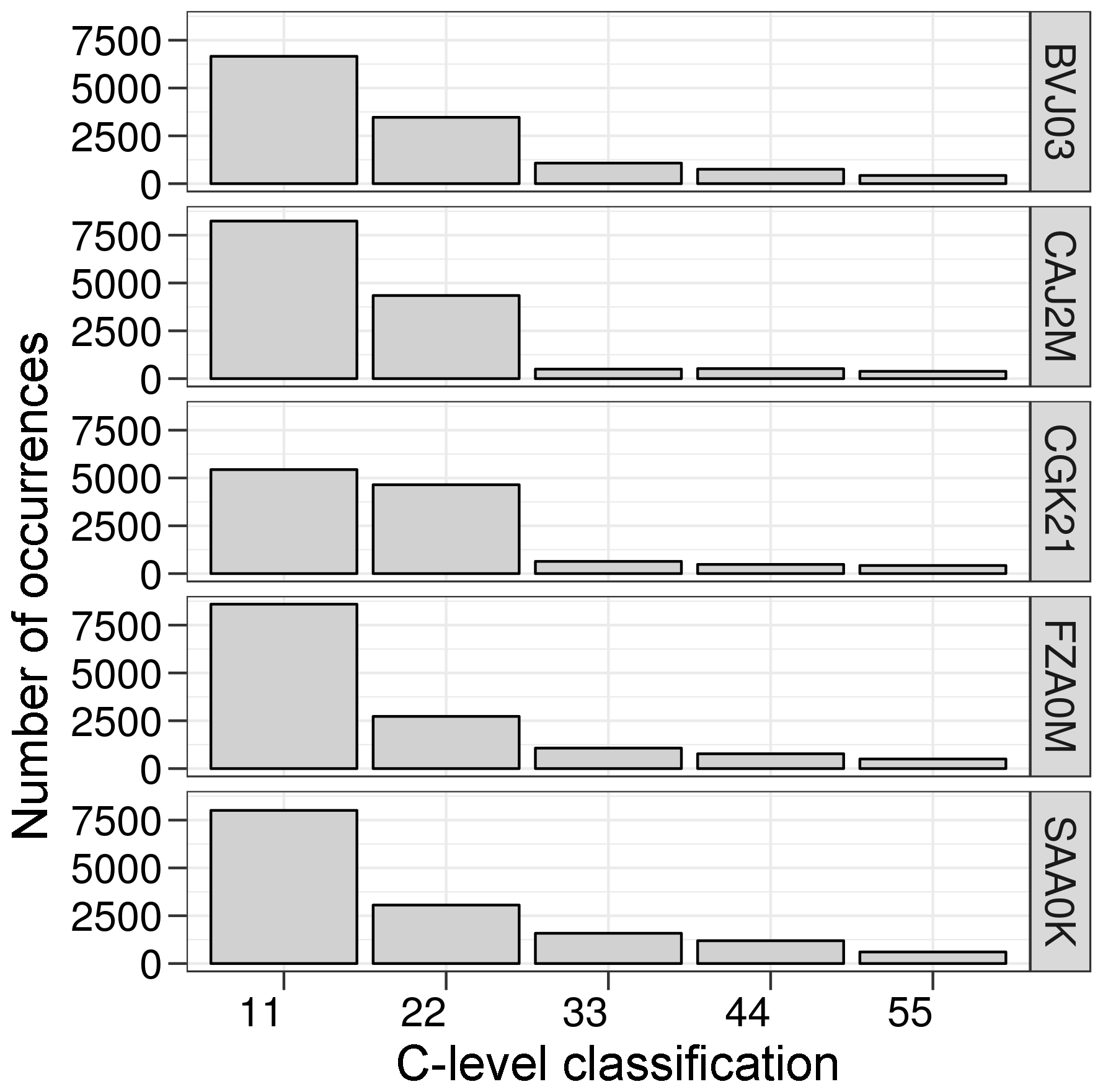
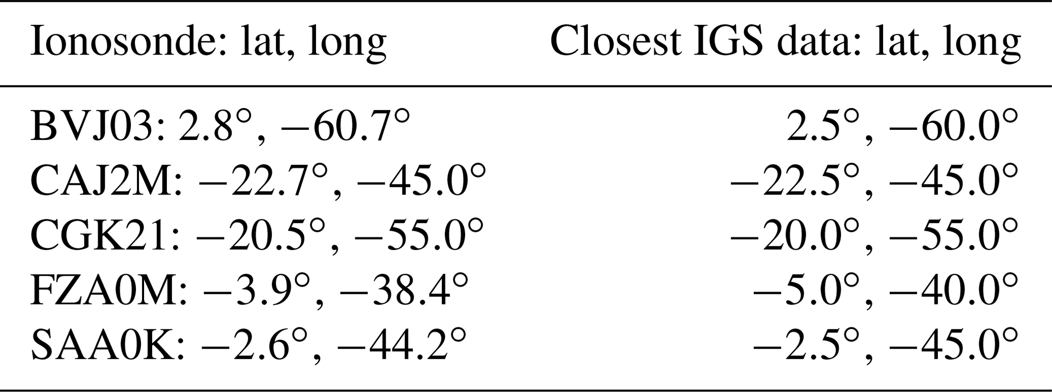
Table 2Ionosonde locations and correspondent closest IGS grid data location.
Ionosonde data were obtained from the INPE database using files in SAO format (version 4) and scaled by the ARTIST auto-scaling system (version 5). Data from up to five instruments (see Fig. 1) were available at the same time for the period considered (2016–2017). Although ionosondes can generate ionograms in less than 10 min intervals, a 1 h interval between soundings was considered in this work, except for the comparisons with IGS data. In that case, a 2 h interval is used to match IGS data availability.
C-Level values were extracted from all ionograms, and despite auto-scaled ionosonde data with a CS above 40 able to be considered acceptable (Galkin et al., 2013), we chose to use only those achieving a CS above 60, corresponding to C-Levels 11 and 22. Figure 2 shows the total number of C-Level flag occurrences for the available data. Figure 3 shows the same distribution, however, considering each ionosonde station separately. It can be seen from Figs. 2 and 3 that the majority of C-Level flag occurrences are in classification levels 11 or 22. Also, more than half of C-Level flags achieve a CS above 80 (C-Level 11).
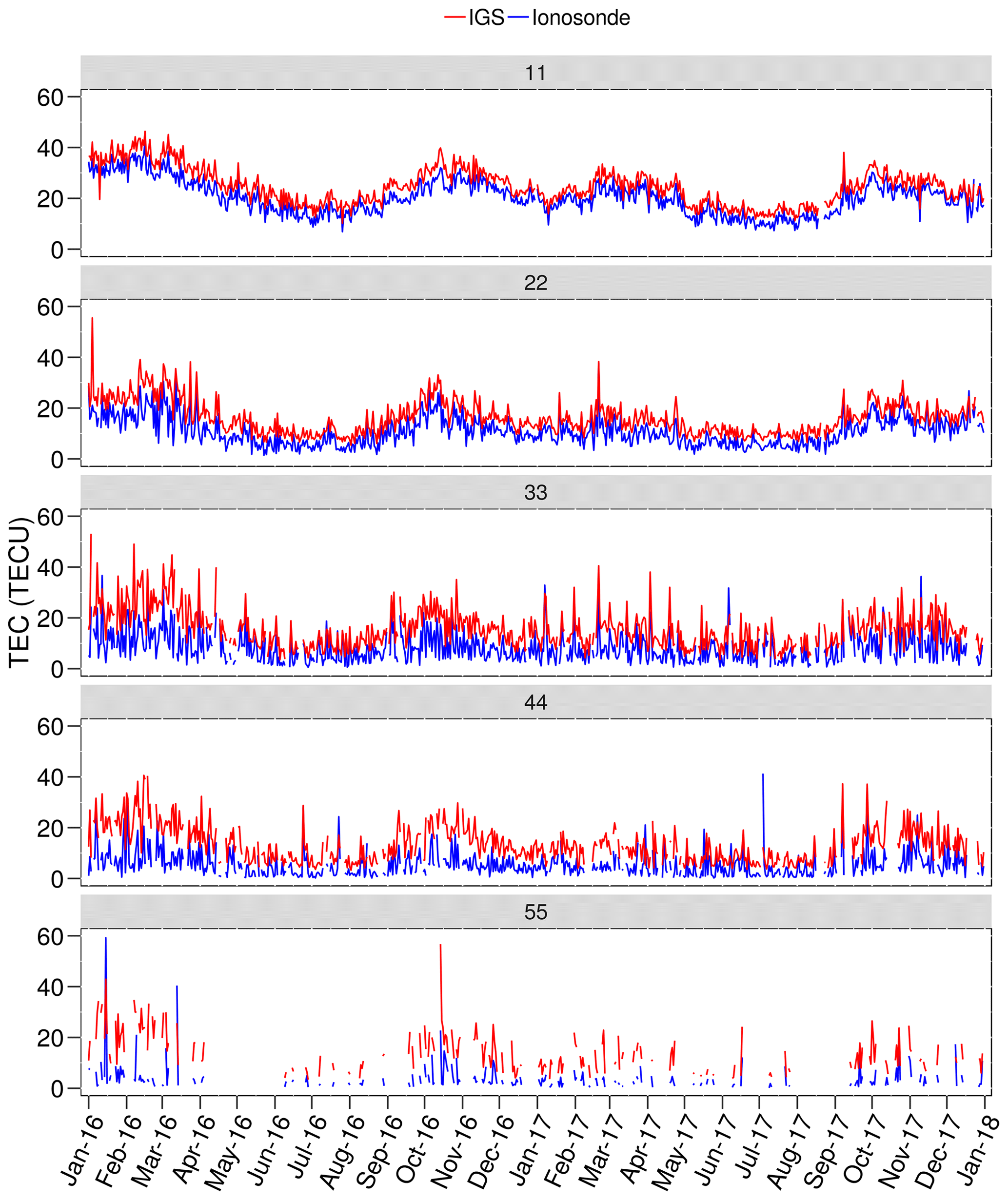
Figure 5vTEC and ITEC daily mean variation for the period under analysis considering the mean value for each C-Level flag classification.
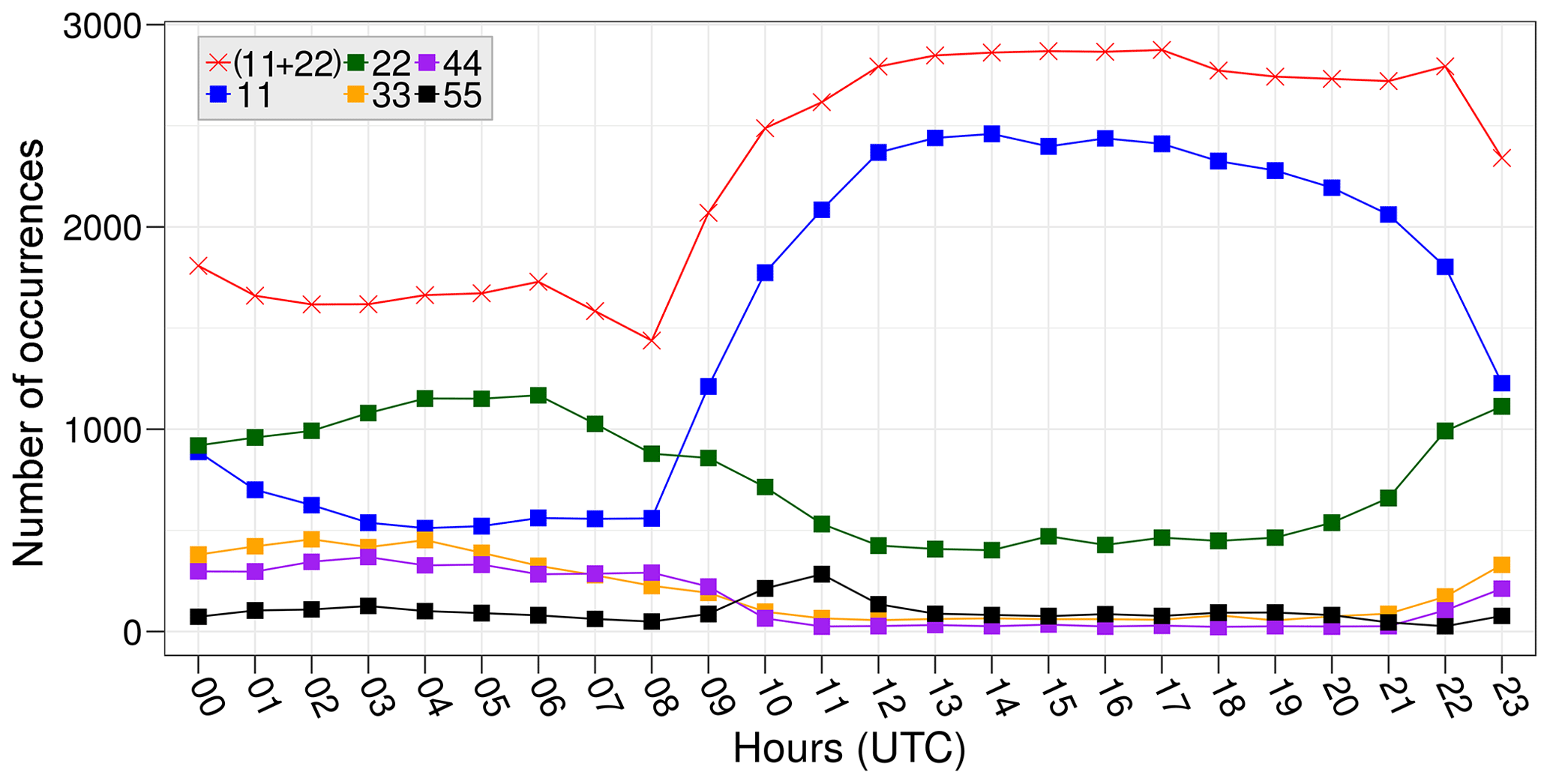
Considering the daily variation in ionosphere electron density, it would be interesting to analyze also the ionosondes' data quality variation within daytime hours taking into account all available data. In Fig. 4 the increase in the occurrence of C-Level 11 after sunset can be seen, while C-Level 22 decreases. The aggregation of C-Level flags 11 and 22 ionograms (used in this work) provides ionosonde data with over 1000 samples even for the period with low occurrences – see the red curve in Fig. 4.
TEC values from IGS maps and ionosondes were compared at the same date or time using the closest geographic correspondence as shown in Table 2, considering the IGS data grid (5∘ in longitude per 2.5∘ in latitude, every 2 h). The analysis is mainly based on the accumulation of TEC differences by applying the root mean squared error (RMSE) as defined in Eq. (1) (Chai and Draxler, 2014):
where errors ei are the differences (with ) between TEC values from the IGS and ionosonde, and n is the total number of values considered.
Ionospheric total electron content (ITEC) daily variability for each ionosonde C-Level flag is shown in Fig. 5, and for each ionosonde station separately, considering only C-Level flags 11 and 22, it is shown in Fig. 6. Since the daily mean ITEC values from flags 11 and 22 follow the IGS vTEC data variation, they are coherent. On the other hand, it can be seen that the vTEC values are consistently higher than ITEC for the whole period and for every ionosonde. In Fig. 5, a noisy and incoherent TEC variation for flags greater than 22 in both vTEC and ITEC is noticeable. Obviously, since the results for flags greater than 22 have low confidence, they may have errors, but this reason can not be used to explain the noise in vTEC values. The data representative of higher flags is low; i.e., there is a reduced number of points and heterogeneous distributions during daytime and nighttime. Such unbalanced distribution can produce daily mean TEC representing only daytime or nighttime that during consecutive days leads to noisy curves.
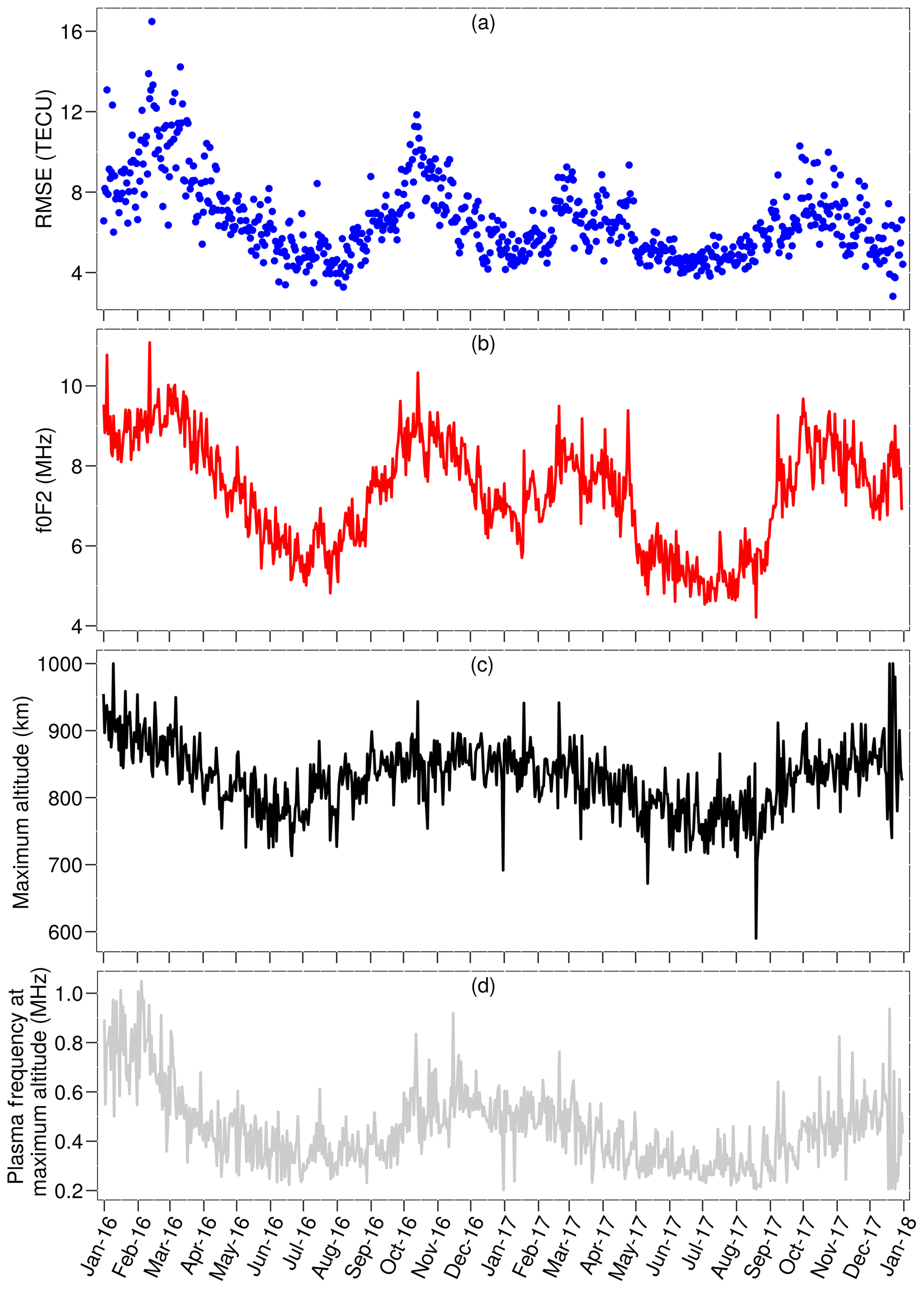
Figure 7Daily mean, considering all ionosondes: (a) ITEC and IGS vTEC differences in terms of RMSE; (b) F2 layer critical frequency; (c) maximum altitude of density profile; and (d) plasma frequency at maximum altitude.
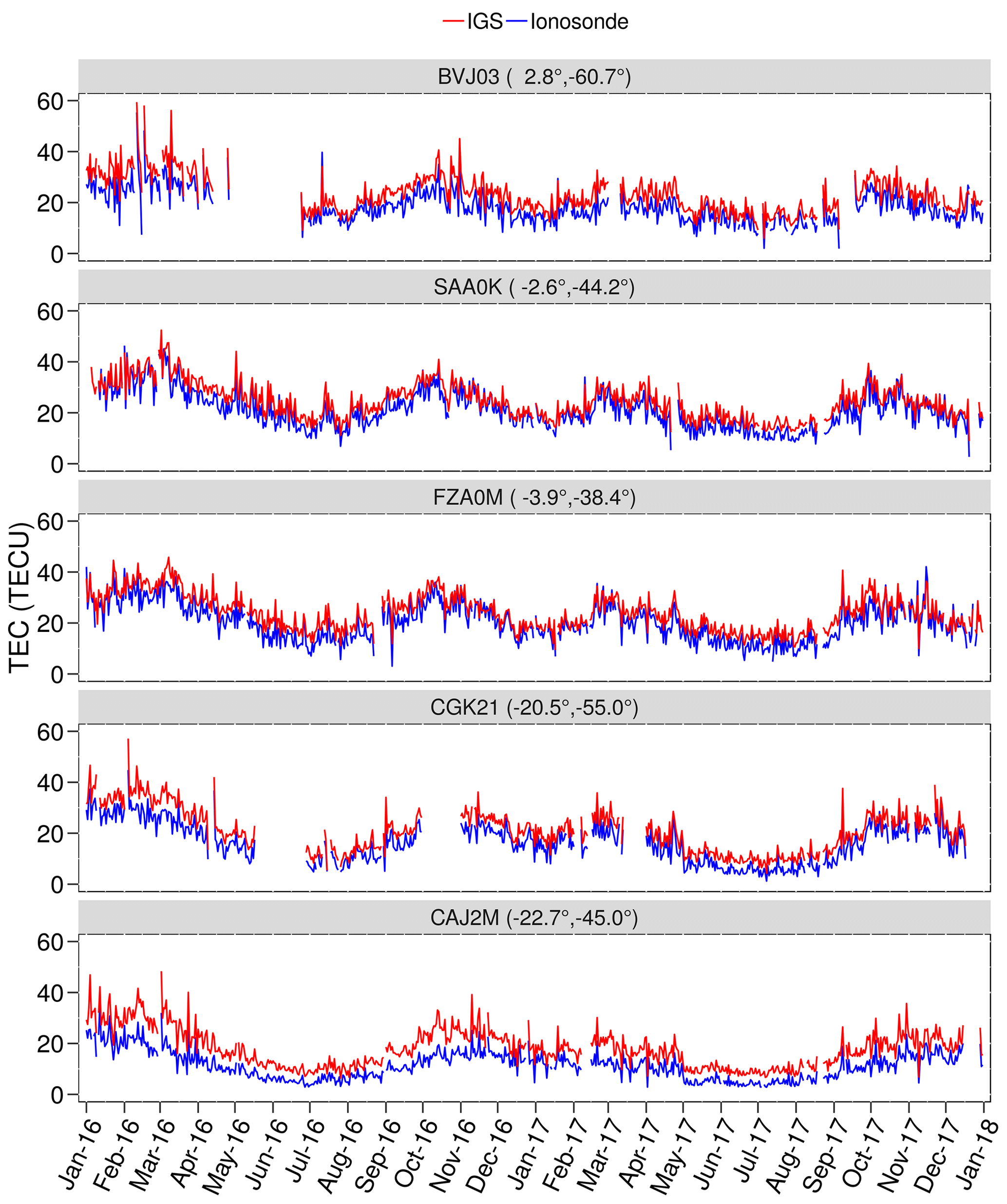
In Fig. 6 we can observe that some ionosondes presented a lack of data for a few days or even entire months. The seasonal variation in ITEC was similar for all stations. During the autumn and winter seasons in the Southern Hemisphere we can notice a decrease in ITEC values for both years evaluated.
All the panels in Fig. 7 present daily mean values, considering the density profiles of all ionosondes. In panel (a) the RMSE when comparing ITEC and IGS vTEC is shown. The seasonal variability in TEC differences seems highly correlated with the ionization distribution along the analyzed period. Figure 7b shows the peak of plasma frequency (foF2), and we can observe the periods of high foF2 values corresponding to high RMSE. The maximum altitude used for electron density integration in ionosondes (Fig. 7c) does not change significantly, rarely reaching 900 km. Figure 7d shows the plasma frequency at the maximum altitude of the density profile, which indicates the level from where it is necessary to extend the ionosphere structure evaluation to higher altitudes. Considering the fixed scale height used in digisonde topside profile modeling, such a contribution has not been included in the ITEC calculation, since values of electron density decay too rapidly above ∼800 km, and the simple extension of maximum integration altitude is insufficient for proper comparisons to IGS vTEC. This is the main reason why the ITEC values from ionosondes are underestimated when compared to IGS values. It is well known that vTEC values from the IGS data represent the integrated electron density along the signal path between the receiver and the satellite altitude (∼ 20 000 km). Thus, this analysis is in agreement with what is shown in Figs. 5 and 6.
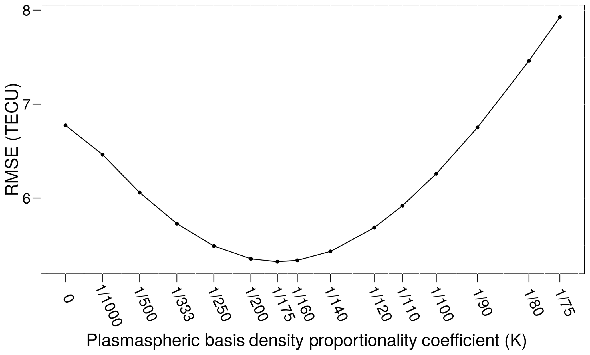
Figure 8Variation of total RMSE with plasmaspheric basis density proportionality coefficient.

Figure 9Daily mean, considering all ionosondes, of ITEC (blue), IGS vTEC (red), and density profile integration up to 20 000 km with topside reconstruction using adapted α-Chapman (orange) and NeQuick formulation (green).
Different analytical functions have been used to model the topside ionospheric density profile (e.g., exponential, Epstein, Chapman) (Nsumei et al., 2012; Pignalberi et al., 2018a; Reinisch et al., 2007). These functions and their variations may adopt fixed or variable scale height. In this work, the ionogram topside profiles were re-modeled using two different approaches that consider fixed and variable scale heights: an adapted α-Chapman exponential decay (Jakowski, 2005) that includes an optimized transition function between the F2 layer and plasmasphere and the NeQuick topside formulation with modeled scale height as a function of a corrected version of the empirical parameter H0 (Pezzopane and Pignalberi, 2019).
3.1 Adapted α-Chapman
The adapted α-Chapman introduced by Jakowski (2005) defines the topside profile NT as
The ionograms provided F2 scale height HT, the electron peak density NmF2 that can be derived from measured critical frequency foF2 using , and peak height hmF2. According to Jakowski (2005), the plasmaspheric scale height Hp can be defined as 10 000 km and the plasmaspheric basis density NP0 is assumed to be proportional to NmF2, i.e., . Using the topside reconstruction of the density profile shown above, the maximum integration height used to estimate ionosonde TEC values was defined as 20 000 km, corresponding to an approximation for the satellite orbit.
In this work, different values for the proportionality coefficient K are examined, and the optimal factor that minimizes the global RMSE is used. Figure 8 shows the ionosonde TEC differences to IGS vTEC in terms of the mean RMSE in the whole period, considering all ionosondes. When K is set to zero, Eq. (2) is reduced to regular α-Chapman decay, and the plasmaspheric slowly decaying exponential term is ignored. As K increases, the underestimated ionosonde TEC values move closer to IGS, hence reducing RMSE. However, after an optimal K, in this experiment equal to 1∕175, the plasmaspheric contribution is exceeded, increasing again RMSE.
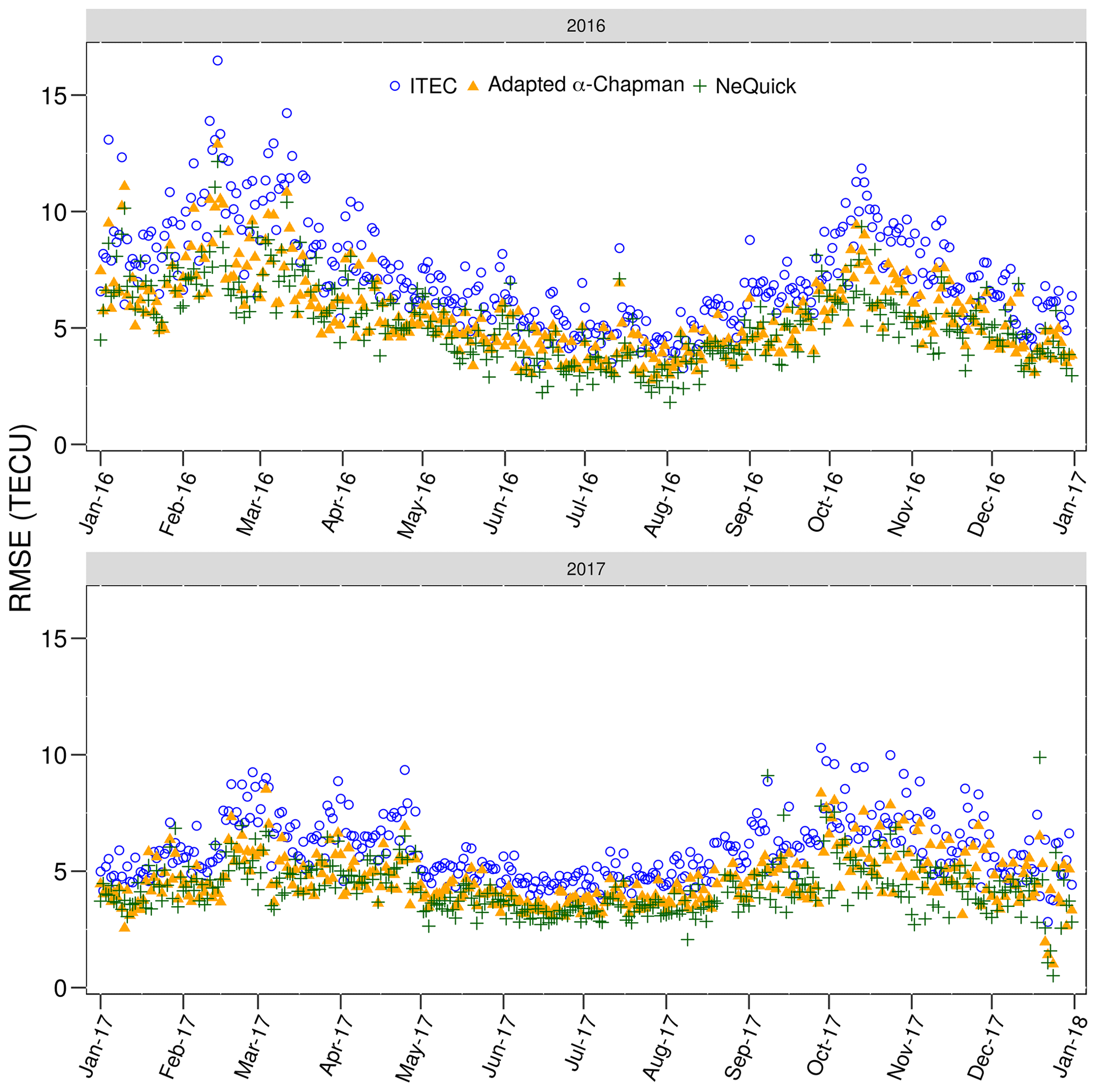
Figure 10Daily mean RMSE variation, considering all ionosondes, for ITEC (blue circle), adapted α-Chapman (orange triangle), and NeQuick topside formulation (green cross).
3.2 NeQuick topside formulation
The NeQuick topside analytical formulation (Nava et al., 2008; Pezzopane and Pignalberi, 2019) is based on a semi-Epstein layer describing the topside electron density profile NT as
In this approach, the modeled scale height HT is dependent on height h, hmF2, and also on the empirical parameter H0:
H0 can be calculated using NmF2, foF2, the propagation factor (M(3000)F2), hmF2, and the smoothed sunspot number (R12) as presented by Nava et al. (2008). Pezzopane and Pignalberi (2019) proposed a new formulation for H0 based on electron density measurements made by the Swarm satellite constellation. The formulation is
where two 2-D grids provide the values of H0,AC and H0,B as a function of foF2 and hmF2. Specifically, the grids have been calculated as the median values obtained by using the NeQuick topside formulation, IRI UP modeled values (Pignalberi et al., 2018b, c), Swarm A and C (for H0,AC), or Swarm B (for H0,B) electron density measurements (Pezzopane and Pignalberi, 2019). In our experiments, hmF2 and foF2 were obtained from the post-processed ionograms and H0,AC and H0,B grids were generously provided by Michael Pezzopane and Alessio Pignalberi from the Istituto Nazionale di Geofisica e Vulcanologia, Italy.
3.3 Comparative evaluation
Figure 9 presents a comparison, considering all ionosondes, among the daily mean ITEC (in blue), IGS vTEC (in red), and density profile integration up to 20 000 km with topside reconstruction using an adapted α-Chapman function (in orange) and a NeQuick formulation (in green). The results are for the years 2016 (top panel) and 2017 (bottom panel). All calculated values follow the reference, i.e., the IGS vTEC variations showing a semi-annual dependency with a minimum in June solstice as well as the day-to-day variability. Indeed, the TEC values obtained with the optimization of an adapted α-Chapman are very similar to the ones from the NeQuick topside procedure, and both are much closer to IGS vTEC than ITEC values.
To identify the best methodology to estimate the plasmaspheric TEC, the daily mean RMSE variation shown in Fig. 10 can be assessed. The differences to IGS vTEC using adapted α-Chapman (orange triangle) and NeQuick (green cross) approaches can be compared to the ITEC errors (blue circle) as shown in Fig. 7a. In general, the RMSE values calculated with adapted α-Chapman and NeQuick are similar. However, the lowest RMSE values along the 2 years 2016 and 2017 belong to the NeQuick criterion, as shown in Fig. 10. In addition, the mean RMSE for the whole period, using adapted α-Chapman reconstruction with the proportionality coefficient optimization, has a minimum value of 5.32 TECU, while using NeQuick topside reconstruction the error is 5.05 TECU.
This paper presented a 2-year period validation of ionosonde data, using IGS vTEC as a reference. Ionogram electron density profiles were first selected based on the confidence score and then integrated in height. As expected, ITEC values were systematically underestimated, which is consistent with an ionospheric topside modeling limitation that uses a fixed scale height, which almost neglects plasma above ∼800 km, while IGS data consider electron densities from the GNSS stations up to the satellite. This claim was supported by the examination of Figs. 5, 6, and 7. The ionogram topside profiles were re-modeled using two different approaches: optimization of an adapted α-Chapman exponential decay and the NeQuick topside formulation, based on a semi-Epstein layer with modeled scale height as a function of a corrected version of the H0 empirical parameter. The electron density integration height was extended to an approximation of satellite orbits. Hence, as expected, for both topside reconstructions the plasmaspheric ionization contribution brought ionosonde TEC values closer to IGS observations. In our experiments, the improvement was significant for determining TEC using ionosonde data, as shown in Figs. 9 and 10. Although both procedures for calculating plasmaspheric TEC yield similar results, the NeQuick criterion shows lower RMSE values, as we can clearly see in Fig. 10.
IGS vTEC maps have been provided by NASA through ftp://cddis.gsfc.nasa.gov/gnss/products/ionex (NASA, 2020). Ionosonde data have been provided by INPE through http://www2.inpe.br/climaespacial/SWMonitorUser/ (EMBRACE, 2020), after a previous registration at http://www2.inpe.br/climaespacial/SWMonitorUser/faces/register.xhtml (last access: 12 February 2020). The 2-D grids for NeQuick topside formulation were provided by Michael Pezzopane (michael.pezzopane@ingv.it) and Alessio Pignalberi (alessio.pignalberi@ingv.it) from the Istituto Nazionale di Geofisica e Vulcanologia.
TdSK assisted in conceiving the study, led the implementation of data processing and analysis, and actively contributed to the discussion of results and paper writing. AP proposed the study, assisted with data processing and analysis, and actively contributed to the discussion of results and paper writing. JRdS assisted in conceiving the study and actively contributed to the discussion of results and paper writing. GSF assisted with data acquisition and manuscript writing. ERdP and HFdCV assisted in discussing the results and reviewing the manuscript.
The authors declare that they have no conflict of interest.
This article is part of the special issue “7th Brazilian Meeting on Space Geophysics and Aeronomy”. It is a result of the Brazilian Meeting on Space Geophysics and Aeronomy, Santa Maria/RS, Brazil, 5–9 November 2018.
The authors would like to acknowledge the Crustal Dynamics Data Information System (CDDIS), NASA Goddard Space Flight Center, Greenbelt, MD, USA, for providing online access to IGS vTEC data. The authors thank the Embrace/INPE program from MCTIC for providing ionosonde data for this work. The authors thank Michael Pezzopane and Alessio Pignalberi from the Istituto Nazionale di Geofisica e Vulcanologia, Italy, for providing a deeper understanding regarding the implementation of the NeQuick topside formulation and access to median values of H0,AC and H0,B as a function of foF2 and hmF2.
Telmo dos Santos Klipp would like to thank the Conselho Nacional de Desenvolvimento Científico e Tecnológico (CNPq, Brazil) for the Programa de Capacitação Institucional PCI-DC research sponsorship (grant no. 300487/2019-3). Gabriel Sandim Falcão acknowledges the CNPq for a PIBIC sponsorship. Jonas Rodrigues de Souza and Eurico Rodrigues de Paula are grateful for funding from the CNPq (grant nos. 307181/2018-9 and 310802/2015-6, respectively) via a research productivity sponsorship and the INCT GNSS-NavAer, which is supported by the CNPq (grant no. 465648/2014-2), FAPESP (grant no. 2017/50115-0), and CAPES (grant no. 88887.137186/2017-00). Haroldo Fraga de Campos Velho would like to thank CNPq for a research productivity sponsorship.
This paper was edited by Inez Batista and reviewed by two anonymous referees.
Bamford, R. A., Stamper, R., and Cander, L. R.: A comparison between the hourly autoscaled and manually scaled characteristics from the Chilton ionosonde from 1996 to 2004, Radio Sci., 43, RS1001, https://doi.org/10.1029/2005RS003401, 2008. a
Chai, T. and Draxler, R. R.: Root mean square error (RMSE) or mean absolute error (MAE)? – Arguments against avoiding RMSE in the literature, Geosci. Model Dev., 7, 1247–1250, https://doi.org/10.5194/gmd-7-1247-2014, 2014. a
EMBRACE: Ionosonde products, available at: http://www2.inpe.br/climaespacial/SWMonitorUser/, last access: 12 February 2020. a
Enell, C.-F., Kozlovsky, A., Turunen, T., Ulich, T., Välitalo, S., Scotto, C., and Pezzopane, M.: Comparison between manual scaling and Autoscala automatic scaling applied to Sodankylä Geophysical Observatory ionograms, Geosci. Instrum. Method. Data Syst., 5, 53–64, https://doi.org/10.5194/gi-5-53-2016, 2016. a
Galkin, I., Reinisch, B. W., Huang, X., and Khmyrov, G. M.: Confidence Score of ARTIST-5 Ionogram Autoscaling, Tech. rep., Ionosonde Network Advisory Group (INAG), INAG Tech. Memorandum, available at: http://www.ursi.org/files/CommissionWebsites/INAG/web-73/confidence_score.pdf (last access: 12 February 2020), 2013. a, b, c, d, e
Galkin, I. A.: Standard Archiving Output (SAO) Format, University of Massachusetts Lowell, 600 Suffolk Street, Lowell, MA 01854, USA, available at: ftp://ftp.ngdc.noaa.gov/STP/ionosonde/documentation/SAO%20version%204.2.pdf (last access: 12 February 2020), 2006. a
Galkin, I. A. and Reinisch, B. W.: The new ARTIST 5 for all digisondes, Ionosonde Network Advisory Group Bulletin, 69, 1–8, available at: http://www.ursi.org/files/CommissionWebsites/INAG/web-69/2008/artist5-inag.pdf (last access: 12 February 2020), 2008. a
Gilbert, J. D. and Smith, R. W.: A comparison between the automatic ionogram scaling system ARTIST and the standard manual method, Radio Sci., 23, 968–974, https://doi.org/10.1029/RS023i006p00968, 1988. a
Hernández-Pajares, M., Juan, J. M., Sanz, J., Orus, R., Garcia-Rigo, A., Feltens, J., Komjathy, A., Schaer, S. C., and Krankowski, A.: The IGS VTEC maps: a reliable source of ionospheric information since 1998, J. Geodesy, 83, 263–275, https://doi.org/10.1007/s00190-008-0266-1, 2009. a, b, c
Huang, X. and Reinisch, B. W.: Vertical electron content from ionograms in real time, Radio Sci., 36, 335–342, https://doi.org/10.1029/1999RS002409, 2001. a
Jakowski, N.: Ionospheric GPS radio occultation measurements on board CHAMP, GPS Solut., 9, 88–95, https://doi.org/10.1007/s10291-005-0137-7, 2005. a, b, c, d, e
Jiang, C., Yang, G., Lan, T., Zhu, P., Song, H., Zhou, C., Cui, X., Zhao, Z., and Zhang, Y.: Improvement of automatic scaling of vertical incidence ionograms by simulated annealing, J. Atmos. Sol.-Terr. Phy., 133, 178–184, https://doi.org/10.1016/j.jastp.2015.09.002, 2015. a
Jin, S. and Jin, R.: GPS Ionospheric Mapping and Tomography: A case of study in a geomagnetic storm, in: Proceeding of IEEE Int. Geosci. and Remote Se., 24–29 July 2011, Vancouver, Canada, 1127–1130, 2011. a
McNamara, L. F.: Quality figures and error bars for autoscaled Digisonde vertical incidence ionograms, Radio Sci., 41, RS4011, https://doi.org/10.1029/2005RS003440, 2006. a
NASA: Ionex products, available at: ftp://cddis.gsfc.nasa.gov/gnss/products/ionex, last access: 12 February 2020. a
Nava, B., Coïsson, P., and Radicella, S.: A new version of the NeQuick ionosphere electron density model, J. Atmos. Sol.-Terr. Phy., 70, 1856–1862, https://doi.org/10.1016/j.jastp.2008.01.015, 2008. a, b
Nsumei, P., Reinisch, B. W., Huang, X., and Bilitza, D.: New Vary-Chap profile of the topside ionosphere electron density distribution for use with the IRI model and the GIRO real time data, Radio Sci., 47, RS0L16, https://doi.org/10.1029/2012RS004989, 2012. a
Pezzopane, M. and Pignalberi, A.: The ESA Swarm mission to help ionospheric modeling: a new NeQuick topside formulation for mid-latitude regions, Sci. Rep.-UK, 9, 12253, https://doi.org/10.1038/s41598-019-48440-6, 2019. a, b, c, d, e
Pezzopane, M. and Scotto, C.: Automatic scaling of critical frequency foF2 and MUF (3000) F2: A comparison between Autoscala and ARTIST 4.5 on Rome data, Radio Sci., 42, RS4003, https://doi.org/10.1029/2006RS003581, 2007. a
Pezzopane, M., Pillat, V. G., and Fagundes, P. R.: Automatic scaling of critical frequency foF2 from ionograms recorded at São José dos Campos, Brazil: a comparison between Autoscala and UDIDA tools, Acta. Geophys., 65, 173–187, https://doi.org/10.1007/s11600-017-0015-z, 2017. a
Pignalberi, A., Pezzopane, M., and Rizzi, R.: Modeling the Lower Part of the Topside Ionospheric Vertical Electron Density Profile Over the European Region by Means of Swarm Satellites Data and IRI UP Method, Space Weather, 16, 304–320, https://doi.org/10.1002/2017SW001790, 2018a. a
Pignalberi, A., Pezzopane, M., Rizzi, R., and Galkin, I.: Effective solar indices for ionospheric modeling: a review and a proposal for a real-time regional IRI, Surv. Geophys., 39, 125–167, https://doi.org/10.1007/s10712-017-9438-y, 2018b. a
Pignalberi, A., Pietrella, M., Pezzopane, M., and Rizzi, R.: Improvements and validation of the IRI UP method under moderate, strong, and severe geomagnetic storms, Earth Planets Space, 70, 180, https://doi.org/10.1186/s40623-018-0952-z, 2018c. a
Reinisch, B. and Huang, X.: Deducing topside profiles and total electron content from bottomside ionograms, Adv. Space Res., 27, 23–30, https://doi.org/10.1016/S0273-1177(00)00136-8, 2001. a
Reinisch, B., Huang, X., Galkin, I., Paznukhov, V., and Kozlov, A.: Recent advances in real-time analysis of ionograms and ionospheric drift measurements with digisondes, J. Atmos. Sol.-Terr. Phy, 67, 1054–1062, https://doi.org/10.1016/j.jastp.2005.01.009, 2005. a, b
Reinisch, B., Nsumei, P., Huang, X., and Bilitza, D.: Modeling the F2 topside and plasmasphere for IRI using IMAGE/RPI and ISIS data, Adv. Space Res., 39, 731–738, https://doi.org/10.1016/j.asr.2006.05.032, 2007. a
Reinisch, B. W. and Galkin, I. A.: Global ionospheric radio observatory (GIRO), Earth Planets Space, 63, 377–381, 2011. a
Reinisch, B. W. and Xueqin, H.: Automatic calculation of electron density profiles from digital ionograms: 3. Processing of bottomside ionograms, Radio Sci., 18, 477–492, https://doi.org/10.1029/RS018i003p00477, 1983. a
Schaer, S., Gurtner, W., and Feltens, J.: IONEX: The IONosphere Map EXchange Format Version 1, in: Proceedings of the IGS AC workshop, 9–11 February 1998, Darmstadt, Germany, 233–247, 1998. a
Scotto, C. and Pezzopane, M.: A software for automatic scaling of foF2 and MUF (3000) F2 from ionograms, in: Proceedings of URSI XXVIIth General Assembly, 17–24 August 2002, Maastricht, Holland, 2002. a
Scotto, C. and Pezzopane, M.: A method for automatic scaling of sporadic E layers from ionograms, Radio Sci., 42, RS2012, https://doi.org/10.1029/2006RS003461, 2007. a
Stankov, S., Jodogne, J.-C., Kutiev, I., Stegen, K., and Warnant, R.: Evaluation of the automatic ionogram scaling for use in real-time ionospheric density profile specification: Dourbes DGS-256/ARTIST-4 performance, Ann. Geophys.-Italy, 55, 283–291, https://doi.org/10.4401/ag-4976, 2012. a