the Creative Commons Attribution 4.0 License.
the Creative Commons Attribution 4.0 License.
 | 06 Jan 2020
Ionospheric total electron content responses to HILDCAA intervals
Regia Pereira da Silva
Clezio Marcos Denardini
Manilo Soares Marques
Laysa Cristina Araujo Resende
Juliano Moro
Giorgio Arlan da Silva Picanço
Gilvan Luiz Borba
Marcos Aurelio Ferreira dos Santos
The High-Intensity Long-Duration and Continuous AE Activities (HILDCAA) intervals are capable of causing a global disturbance in the terrestrial ionosphere. However, the ionospheric storms' behavior due to these intervals is still not widely understood. In the current study, we seek to comprise the HILDCAA disturbance time effects in the total electron content (TEC) values with respect to the quiet days' pattern by analyzing local time and seasonal dependences, and the influences of the solar wind velocity on a sample of 10 intervals that occurred in the years 2015 and 2016. The main results showed that the hourly distribution of the disturbance TEC may vary substantially between one HILDCAA interval and another. An equinoctial anomaly was found since the equinoxes represent more ionospheric TEC responses than the solstices. Regarding the solar wind velocities, although HILDCAA intervals are associated with high-speed streams, this association does not present a direct relation to TEC disturbance magnitudes at low and equatorial latitudes.
- Article
(1834 KB) - Full-text XML
- BibTeX
- EndNote


Similarly to geomagnetic storms, High-Intensity Long-Duration and Continuous AE Activities (HILDCAA) intervals can influence the ionosphere, leading to disturbances in the ionospheric F2 region. It is well known that these intervals can change the F2-region peak height, being, generally, less intense than those observed during typical geomagnetic storm events (Sobral et al., 2006; Koga et al., 2011; Silva et al., 2017).
In fact, HILDCAAs are characterized by presenting some criteria: (i) the AE index must reach an intensity peak greater than or equal to 1000 nT; (ii) the AE index needs to be almost continuous and never drop below 200 nT for more than 2 h at a time; (iii) the event must have a duration of at least 2 d; and (iv) the event occurred after the main phase of magnetic storms. However, the same physical process may occur when one of the four criteria is not strictly followed (Tsurutani and Gonzalez, 1987; Tsurutani et al., 2004, 2006; Sobral et al., 2006, Hajra et al., 2013, Silva et al., 2017). As the main feature is the high AE index levels, in this study we have considered drops below 200 nT for more than 2 h as long as the AE index value returns in high activity for prolonged hours.
The electron density perturbation in the ionosphere during HILDCAA events is different from the one that occurred during geomagnetic storms in the equatorial and low-latitude stations. Since the HILDCAA presents a weak/moderate geoeffectiveness when compared to the other forms of space disturbances, it is expected that the ionosphere response will present a different behavior.
The total electron content (TEC) is an important ionospheric parameter to several studies and technological applications. As HILDCAAs can cause F2-region peak alterations, enhancements/depletions can be observed in the TEC profile. In fact, the TEC response to the geomagnetic storms is a well-known issue in the space physics field (Lu et al., 2001; Kutiev et al., 2005; Mendillo, 2006; Maruyama and Nakamura, 2007; Biqiang et al., 2007). However, only a few studies about TEC patterns during HILDCAA intervals have been found in the literature (de Siqueira et al., 2011).
Ionospheric storms are manifestations of space weather events, which are caused by energy inputs in the upper atmosphere in the form of enhanced electric fields, currents, and energetic particle precipitation (Buonsanto, 1999; Mendillo, 2006). Usually, ionospheric storms are associated with ionosphere responses to geomagnetic storm events. However, in a broader way, these responses happen due to magnetospheric energy inputs to the Earth's upper atmosphere, and this can occur to all kinds of geomagnetic activity forms. Park (1974) pointed out that ionospheric storms can be understood in terms of the superposed effects of many substorms. In view of this and considering that the development of ionospheric storms during HILDCAA intervals has not been dealt with in depth, in the current study we have focused on the TEC pattern during this kind of event.
Recently, Verkhoglyadova et al. (2013) suggested that HILDCAAs associated with high-speed streams (HSS) can be one of the external driving TEC variabilities. Indeed, the continuous energy injection and energetic particle precipitation into the polar upper atmosphere during HILDCAA intervals could modify the dynamic and chemical coupling process of the thermosphere–ionosphere system, resulting in changes in the electron density. These modifications, beyond changing the auroral electron density, can be mapped to low latitudes involving electric field disturbances, as prompt penetration electric fields (PPEF) and disturbance dynamos (DD) (Koga et al., 2011; Silva et al., 2017; Yeeram and Paratrasri, 2019).
Therefore, in the current study we have focused on the TEC pattern during HILDCAA intervals, taking into account local time dependence, seasonal dependence, and high-/slow-speed stream influences in the equatorial and low-latitude ionosphere. This paper is structured as follows: in the next section we present the HILDCAA intervals chosen to support this study as well as the GNSS receiver locations over the Brazilian region. In Sect. 3 we show the results and discussion of the analysis, and the conclusions are presented in the last section.
In this study it was possible to construct an overall perception of the ionospheric storms that occurred during HILDCAA disturbance time intervals that affect the TEC values with respect to the expected behavior for quiet days. The features studied are local time and seasonal dependences, and solar wind velocity influences.
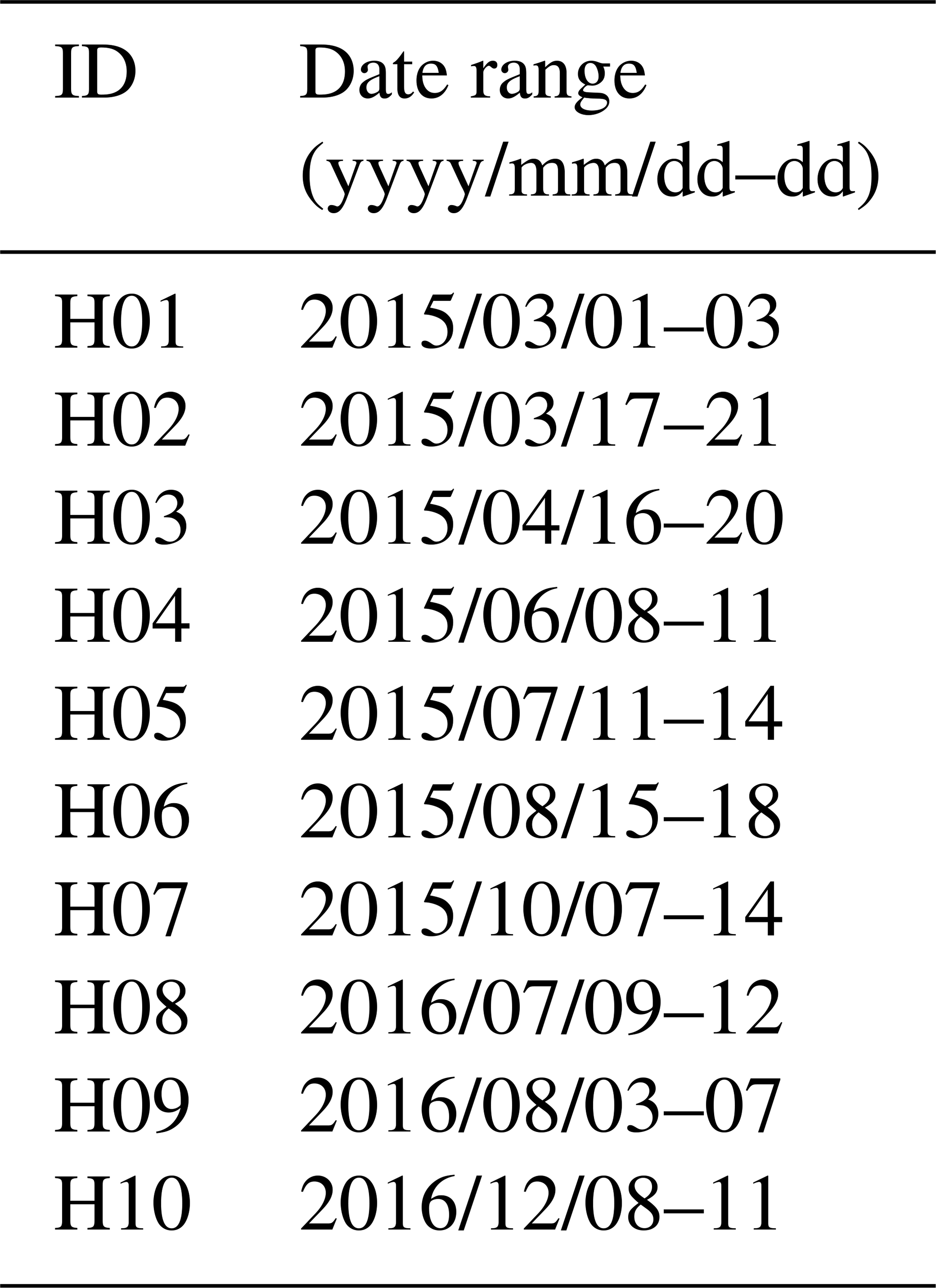
We have selected 10 HILDCAA intervals that occurred during the 2015–2016 period. These intervals are listed in Table 1, where the two columns present the identification and the data range of each interval. The geomagnetic indices and interplanetary data used to classify the HILDCAA events were obtained from OMNIWeb Plus data and service. The Kp index data were obtained from the World Data Center for Geomagnetism, Kyoto, Japan. In this work the daily Kp sum value was used.
Table 1The date range for HILDCAA intervals identified during years 2015–2016.
The TEC mean was initially processed by a program developed at the Institute for Space Research, Boston College, USA (Krishna, 2017). The mean values of vertical TEC (VTEC) were obtained from two Brazilian GNSS stations, São Luís (SL) (2.59∘ S; 44.21∘ W) and Cachoeira Paulista (CP) (22.68∘ S; 44.98∘ W), representing the station closest to the Equator and the low-latitude station, respectively. The Rinex files used in this study were obtained from the Brazilian Network for Continuous Monitoring of the GNSS-RBMC Systems (RBMC). Besides that, the TEC data during HILDCAA events were analyzed and then compared with a set of 3 d averages belonging to a quiet period, in which it refers to the 3 d less disturbed (ΣKp < 24) of the month of the occurrence of each HILDCAA interval.
Figure 1 shows a map with the location of each GNSS station, which is represented by a red triangle. The dashed line represents the magnetic equator. The TEC data obtained during the HILDCAA intervals were analyzed and then compared to the TEC data during the selected quiet days, resulting in dTEC (dTEC = TEC mean − TEC quiet days). All the analyses done in this work took into account the dTEC values.
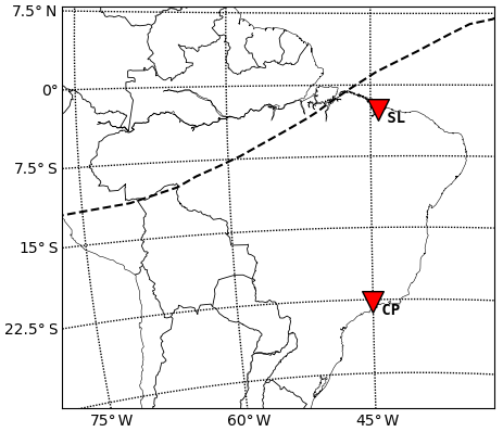
Figure 1Map showing the locations of the GNSS stations used in the present study. Both stations are located in the Brazilian region and are marked by a red triangle, where SL and CP are, respectively, São Luís and Cachoeira Paulista.
In this section, we will present the ionospheric TEC responses observed during 10 HILDCAA intervals focusing on local time dependence and seasonal features and the solar wind velocity influences.
3.1 Local time dependence
A common feature of ionospheric storms is being associated with dependence on local time, mainly when they are caused by geomagnetic storms (Titheridge and Buonsanto, 1988; Pedatella et al., 2010). However, to the best of the authors' knowledge, no study has been found analyzing this aspect when regarding HILDCAA intervals.
Figures 2 and 3 show the mean dTEC hourly values related to all HILDCAA intervals for São Luís and Cachoeira Paulista, respectively. Each panel represents a single interval from the bottom (H01) to the top (H10). The x axis is given in Universal Time (LT = UT − 3) and the color scale represents the dTEC values in TEC units (TECu).
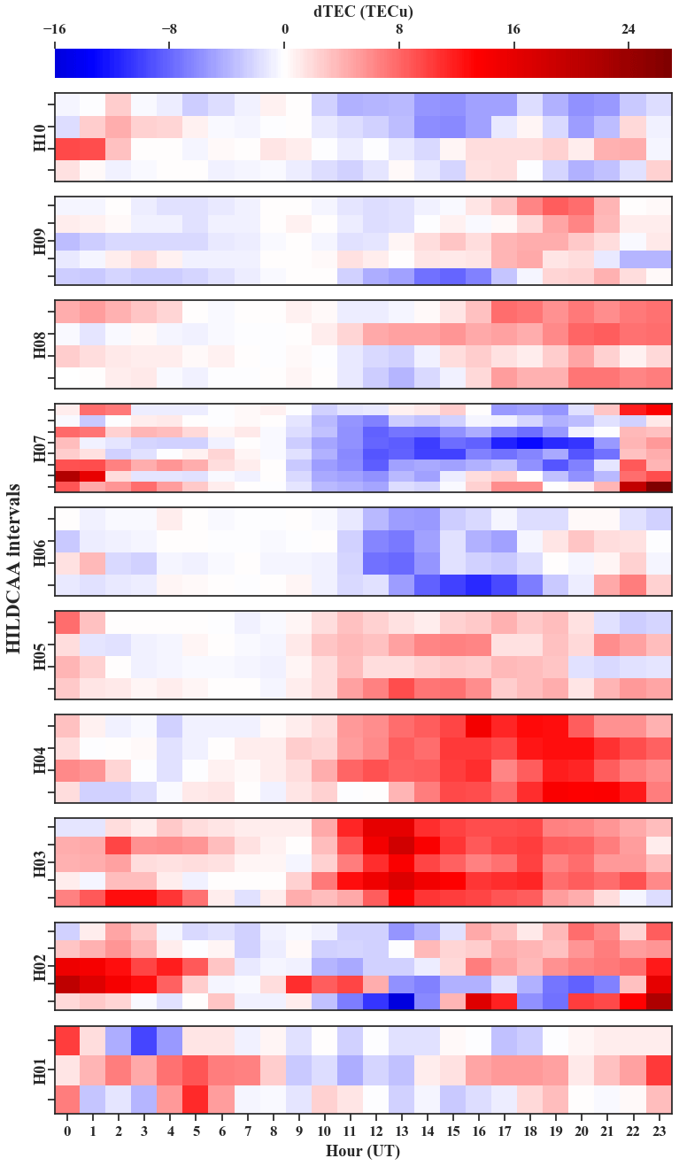
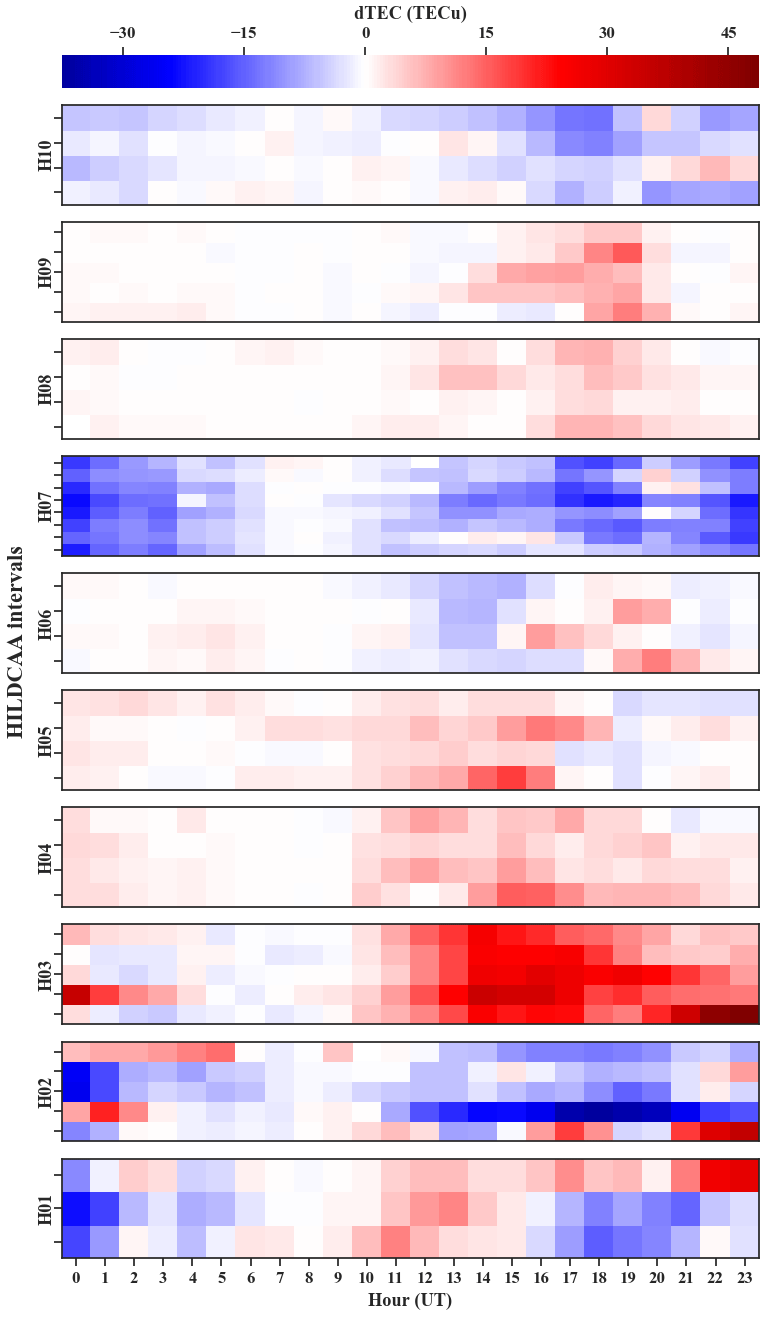
Figure 3dTEC hourly values for all HILDCAA intervals at Cachoeira Paulista (low-latitude station).
Note that the dTEC values have a greater magnitude for the low-latitude GNSS station, to the detriment of the closer equatorial GNSS station. The minimum and maximum values are, respectively, −16.00 and 27.40 TECu for São Luís, and −37.60 and 48.80 TECu for Cachoeira Paulista. These values were considered to perform the TEC hourly distribution; i.e., for each specific GNSS station, the maximum and minimum TEC values were used to analyze all HILDCAAs in the same range. This fact explains why some intervals appear too close to the quiet time pattern. We believed that since the HILDCAA events have low/moderate geoeffectiveness, high values of the dTEC were not expected.
The distribution of the dTEC effects hour-to-hour during HILDCAA intervals shows substantial variability from one event to another. Habarulema et al. (2013) found that the negative storm effects are observed during geomagnetic storm recovery phases over equatorial latitudes. However, since HILDCAA intervals are characterized by a long continuous phase of Dst index recovery, this does not apply. The HILDCAA intervals present the positive dTEC predominance; 60 % (70 %) of all intervals present a positive dTEC response during the whole event for São Luís (Cachoeira Paulista). In a more simplified definition, HILDCAA means an interval where there is always energy injection (Søraas et al., 2004; Sandanger et al., 2005). Silva et al. (2017) observed that during HILDCAA intervals the uplift of the equatorial F2 region peak height was seen, probably due to prompt penetration electric fields. One of the main mechanisms of TEC enhancements is the rise of the ionosphere to higher altitudes where the recombination rates are small. Besides that, our results are in agreement with the results found by de Siqueira et al. (2017). They did a study comparing the TEC responses between two magnetic storms and two HILDCAA intervals following them and found a great TEC variability pattern from one to another event. Hereupon, it was not possible to find a response pattern to the HILDCAA effects in the equatorial and low-latitude TEC considering only the local time. There is great variability, and it is important to consider the day-to-day ionospheric variabilities as well as the separate effect of each electric field disturbance (PPEF/DD).
Comparing both stations, Cachoeira Paulista GNSS station presented higher values to both positive and negative ionospheric storms. During the daytime hours, the latitude is responsible for the different ionospheric responses due to the presence of photoionization. This probably explains the dTEC's higher sensibility to the low-latitude station, to the detriment of the closer equatorial-latitude station.
Analyzing the hourly behavior of each interval from Figs. 2 and 3, we observed more intensity in TEC disturbances for both positive and negative storms, during some specific intervals. This aspect led us to make a seasonal analysis, which will be presented in the next section.
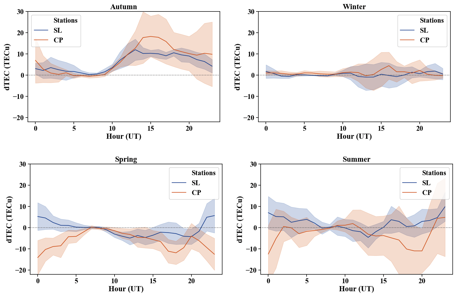
Figure 4Seasonal dTEC response to HILDCAA intervals. The blue and coral lines refer to São Luís and Cachoeira Paulista, respectively.
3.2 Seasonal dependence
It is well known for geomagnetic storms that the influence of the season entails on positive/negative ionospheric storms is more pronounced in winter/summer than in equinox months (Matsushita, 1959; Prölss and Najita, 1975; Mendillo, 2006, among others). However, it has not yet been established whether the occurrence of HILDCAA intervals in different seasons can create different TEC disturbances.
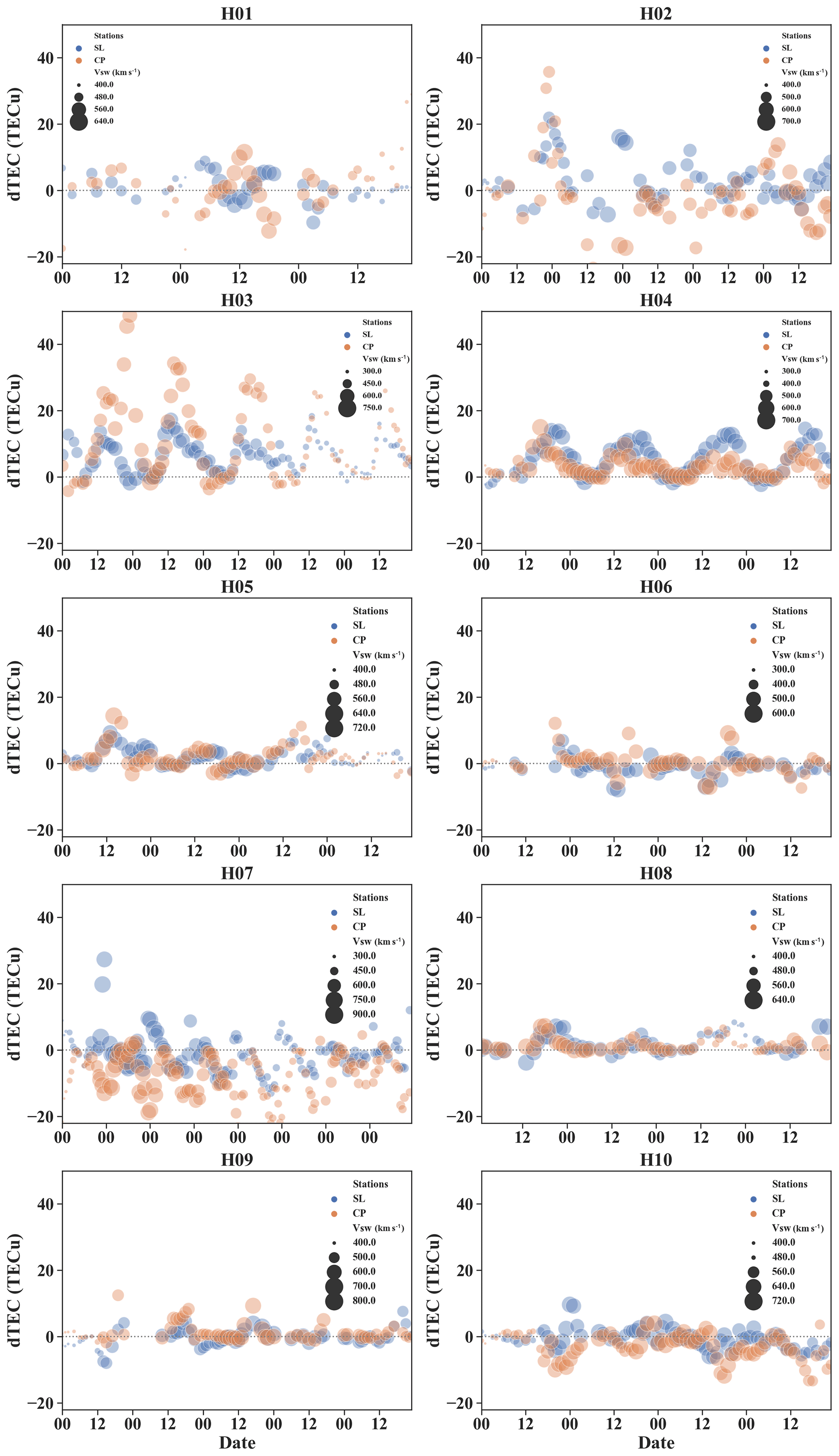
Figure 5Solar wind velocity analysis during HILDCAA intervals. The blue and coral colors refer to São Luís and Cachoeira Paulista stations, respectively, while the bubble diameter is related to velocity (km s−1).
In a recent study involving more than 100 HILDCAA events, Hajra et al. (2013) reported no seasonal dependence with regards to the predominant occurrence rate in any specific epoch of the year due to the solar cycle influences. They announced that the HILDCAAs may occur during any month and any year, with increases in the numbers of events occurring during the solar cycle descending phase. In the current study, it was considered, as seasonal dependence features the TEC disturbance responses at HILDCAA intervals already classified in a seasonal way. The years 2015 and 2016 comprise the descending phase of the 24th solar cycle, which made it possible to catalog an expressive number of HILDCAA events in a short time. Among the 10 intervals chosen for this study, we have separated 8 to represent the seasonal variability, 2 events for each season, taking into account the month of occurrence of each interval and considering the seasons as they occur in the Southern Hemisphere. The intervals are distributed according to Table 2.
Table 2Seasonal classification of HILDCAA intervals (according to the seasons in the Southern Hemisphere).
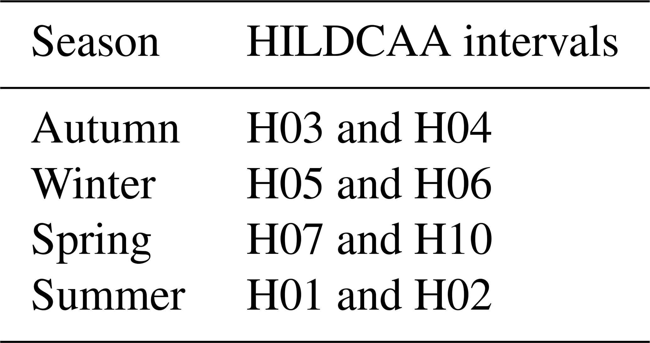
Figure 4 shows the disturbed TEC according to the seasonal classification, which the blue and coral colors refer to São Luís and Cachoeira Paulista, respectively. The solid lines show an estimate of the central tendency for all values, minute-to-minute, for all days of the events belonging to the season, while the shaded area represents the confidence interval for that estimate. While the positive storms are more pronounced in the winter for geomagnetic storms, for HILDCAA intervals this season presents less geoeffectiveness, or almost none. Our results show that the equinoxes represent more ionospheric TEC responses during HILDCAA intervals than the solstices. Both equatorial and low-latitude stations present positive storms during the autumn, while the spring presents a negative behavior, mainly. This equinoctial anomaly may have originated from the equinoctial differences in neutral winds, thermospheric composition, and electric fields. Additional studies are necessary to quantify how each factor can play an important role in HILDCAA seasonal TEC disturbances.
3.3 Solar wind velocity analysis
During the solar cycle descending phase, polar coronal holes migrate to lower latitudes emanating intense magnetic fields. When HSS from these low-latitudinal coronal holes interact with slow speed streams (SSS), a region called Corotating Interaction Regions (CIR) is formed and is well characterized by compressions of the magnetic field and plasma.
There are considerable works that show how HILDCAA is well associated with HSS and CIRs (Tsurutani et al., 2006; Verkhoglyadova et al., 2013). However, to be associated does not necessarily mean that the degree of geoeffectiveness is directly related to high speeds. In addition, Yeeram (2019) suggests that Alfvén waves present during HILDCAA intervals are more dominant than CIR storms, revealing that both are controlled by different interplanetary drivers.
Figure 5 shows the solar wind velocities (VSW) during each HILDCAA interval. As in Fig. 4, the blue and coral colors refer to São Luís and Cachoeira Paulista, respectively. The diameter of the bubble is related to the velocity. The results showed great variability from one interval to another, even considering the intervals that occurred in the same year. In our first analysis (not shown here) we did not find a direct association or cross-correlation between the VSW magnitude and the dTEC in the equatorial and low-latitude GNSS stations. Kim (2007) indicated that HILDCAA intervals can be accompanied by HSS as well as SSS. It is possible to see in our results that the dTEC responses to some intervals present similar behaviors to both HSS and SSS (e.g., H03, H07, and H08). This means that HILDCAA intervals can affect the ionospheric TEC, but not in a direct correlation.
For this work, the ionospheric TEC response to a sample of 10 HILDCAA intervals has been studied. We have used two GNSS stations from the RBMC network representing equatorial and low-latitude locations. As HILDCAA can affect the equatorial ionospheric F2 region, some disturbed TEC from its quiet time pattern is found. Addressing how the ionospheric storms behave during the HILDCAA intervals is our main goal.
In summary, HILDCAA geoeffectiveness on Earth is mainly associated with CIRs; for this reason, the HILDCAA occurrence is more recurrent in the solar cycle descending phase since CIRs play a major role during this phase. Their effects occur during magnetic reconnection due to association with the southward z component of the interplanetary magnetic field and Alfvén waves present in it (Tsurutani et al., 2004). These long-lasting intervals are due to continuous injection of energy and precipitation of particles, which disturb the high-latitude ionosphere. The main disturbances are changes in thermospheric neutral composition, temperature, winds, and electric fields. Similarly to geomagnetic storms, these disturbances can be mapped to low and equatorial latitude and alter the quiet time ionosphere. However, generally, they are less intense because in one astronomical unit the CIRs are not fully developed. In this study we seek to understand the behavior of the ionospheric storm during HILDCAA intervals. The main results are highlighted below.
-
The hourly distribution of the dTEC during HILDCAA intervals may vary substantially between low and equatorial latitudes. The photoionization associated with latitude is probably responsible for these variations.
-
Despite the geomagnetic storms' recovery phase presenting negative ionospheric storms, this pattern does not occur during HILDCAA intervals. There is great variability from one interval to another, but, predominantly, a positive phase occurs.
-
Regarding seasonal features, while the positive storms are more pronounced in the winter for geomagnetic storms, this season presents less geoeffectiveness, or almost none to HILDCAA intervals. The equinoxes represent more ionospheric responses to HILDCAA intervals, presenting positive/negative phase predominance during the autumn/spring.
-
A well-known HILDCAA feature is its association with HSS present in the solar wind. However, this association does not present a direct relation with regards to TEC disturbances at low and equatorial latitudes.
To conclude, the upshot of this study is the possibility of understanding how ionospheric storms behave during some HILDCAA intervals and contributing to improving the discussions about this issue.
The data used in this work are made publicly available on the following sites: https://omniweb.gsfc.nasa.gov/ow.html (last access: 2 January 2020), http://wdc.kugi.kyoto-u.ac.jp/kp/index.html (last access: 13 March 2019), and ibge.gov.br/en/geosciences/geodetic-positioning/ (last access: 13 March 2019). The GPS-TEC program used in this work is available at http://seemala.blogspot.com/ (last access: 13 March 2019).
RPdS conceived the study, designed the data analysis, discussed the results, and led the writing of the manuscript. CMD assisted in conceiving the study, designing the GNSS data analysis, and discussing the final results. MSM assisted with the GNSS data analysis and with designing the figures. LCAR assisted in designing the study and discussing the results of the study. JM assisted in designing the study and discussing the results of the study. GAdSP assisted in discussing the results of the study and reviewing the manuscript. GLB assisted in discussing the results of the study and reviewing the manuscript. MAFdS assisted in discussing the results of the study and reviewing the manuscript. All the authors helped to write and to revise the manuscript.
The authors declare that they have no conflict of interest.
This article is part of the special issue “7th Brazilian meeting on space geophysics and aeronomy”. It is a result of the Brazilian meeting on Space Geophysics and Aeronomy, Santa Maria-RS, Brazil, 5–9 November 2018.
Regia Pereira da Silva acknowledges the support from the Conselho Nacional de Desenvolvimento Científico e Tecnológico (CNPq) through grant 300329/2019-9, and Clezio Marcos Denardini thanks CNPq/MCTIC (grant 303643/2017-0). Laysa Cristina Araújo Resende would like to thank the China-Brazil Joint Laboratory for Space Weather (CBJLSW), National Space Science Center (NSSC), and Chinese Academy of Sciences (CAS), for supporting her postdoctoral work. Juliano Moro would like to acknowledge the China-Brazil Joint Laboratory for Space Weather (CBJLSW), National Space Science Center (NSSC), Chinese Academy of Sciences (CAS), for supporting his postdoctoral fellowship, and the CNPq for grant 429517/2018-01. Giorgio Arlan da Silva Picanço thanks CAPES for supporting his PhD (grant no. 88887.351778/2019-00). We also would like to thank the OMNIWeb Plus data and service and the World Data Center for Geomagnetism, Kyoto. The Rinex files were obtained from the Brazilian Network for Continuous Monitoring of the GNSS-RBMC Systems (RBMC) at interface. The authors acknowledge Gopi Seemala for making available the GPS-TEC program.
This paper was edited by Dalia Buresova and reviewed by Thana Yeeram and Ana G. Elias.
Biqiang, Z., Weixing, W., Libo, L., and Tian, M.: Morphology in the total electron content under geomagnetic disturbed conditions: results from global ionosphere maps, Ann. Geophys., 25, 1555–1568, https://doi.org/10.5194/angeo-25-1555-2007, 2007.
Buonsanto, M. J.: Ionospheric storms – A review, Space Sci. Rev., 88, 563–601, 1999.
de Siqueira, P. M., de Paula, E. R., Muella, M. T. A. H., Rezende, L. F. C., Abdu, M. A., and Gonzalez, W. D.: Storm-time total electron content and its response to penetration electric fields over South America, Ann. Geophys., 29, 1765–1778, https://doi.org/10.5194/angeo-29-1765-2011, 2011.
de Siqueira Negreti, P. M., de Paula, E. R., and Candido, C. M. N.: Total electron content responses to HILDCAAs and geomagnetic storms over South America, Ann. Geophys., 35, 1309–1326, https://doi.org/10.5194/angeo-35-1309-2017, 2017.
Habarulema, J. B., McKinnell, L. A., Burešová, D., Zhang, Y., Seemala, G., Ngwira, C., Chum, J., and Opperman, B.: A comparative study of TEC response for the African equatorial and mid-latitudes during storm conditions J. Atmos. Sol.-Terr. Phys., 102, 105–114, https://doi.org/10.1016/j.jastp.2013.05.008, 2013.
Hajra, R., Echer, E., Tsurutani, B. T., and Gonzalez, W. D.: Solar cycle dependence of High-Intensity Long-Duration Continuous AE Activity (HILDCAA) events, relativistic electron predictors?, J. Geophys. Res., 118, 5626–5638, https://doi.org/10.1002/jgra.50530, 2013.
Kim, H.: Study on the particle injections during HILDCAA intervals, J. Astronom. Space Sci., 24, 119–124, https://doi.org/10.5140/JASS.2007.24.2.119, 2007.
Koga, D., Sobral, J. H. A., Gonzalez, W. D., Arruda, D. C. S., Abdu, M. A., Castilho, V. M., Mascarenhas, M., Gonzalez, A. C., Tsurutani, B. T., Denardini, C. M., and Zamlutti, C. J.: Electrodynamic coupling process between the magnetosphere and the equatorial ionosphere during a 5-day HILDCAA event, J. Atmos. Sol.-Terr. Phys. 73, 148–155, https://doi.org/10.1016/j.jastp.2010.09.002, 2011.
Krishna, S. G.: GPS-TEC Analysis Software Version 2.9.5, available at: http://seemala.blogspot.in/ (last access: 13 March 2019), 2017.
Kutiev, I., Watanabe, S., Otsuka, Y., and Saito, A.: Total electron content behavior over Japan during geomagnetic storms, J. Geophys. Res., 110, A1, https://doi.org/10.1029/2004JA010586, 2005.
Lu, G., Richmond, A. D., Roble, R. G., and Emery, B. A.: Coexistence of ionospheric positive and negative storm phases under northern winter conditions: A case study, J. Geophys. Res., 106, 24493–24504, https://doi.org/10.1029/2001JA000003, 2001.
Maruyama, T. and Nakamura, M.: Conditions for intense ionospheric storms expanding to lower midlatitudes, J. Geophys. Res., 112, A5, https://doi.org/10.1029/2006JA012226, 2007.
Matsushita, S.: A study of the morphology of ionospheric storms, J. Geophys. Res., 64, 305–321, https://doi.org/10.1029/JZ064i003p00305, 1959.
Mendillo, M.: Storms in the ionosphere: Patterns and processes for total electron content, Rev. Geophys., 44, 4, https://doi.org/10.1029/2005RG000193, 2006.
Park, C. G.: A morphological study of substorm-associated disturbances in the ionosphere, J. Geophys. Res., 79, 2821–2827, https://doi.org/10.1029/JA079i019p02821, 1974.
Pedatella, N. M., Lei, J., Thayer, J. P., and Forbes, J. M.: Ionosphere response to recurrent geomagnetic activity: Local time dependency, J. Geophys. Res.-Space, 115, A2, https://doi.org/10.1029/2009JA014712, 2010.
Prölss, G. W. and Najita, K.: Magnetic storm associated changes in the electron content at low latitudes, J. Atmos. Terr. Phys., 37, 635–643, https://doi.org/10.1016/0021-9169(75)90058-6, 1975.
Sandanger, M. I., Søraas, F., Aarsnes, K., Oksavik, K., Evans, D. S., and Greer, M. S.: Proton Injections Into the Ring Current Associated With B∼z Variations During Hildcaa Events, Geophys. Monogr.-Am. Geophys. Union, 155, 249, https://doi.org/10.1029/155GM26, 2005.
Silva, R. P., Sobral, J. H. A., Koga, D., and Souza, J. R.: Evidence of prompt penetration electric fields during HILDCAA events, Ann. Geophys., 35, 1165–1176, https://doi.org/10.5194/angeo-35-1165-2017, 2017.
Sobral, J. H. A., Abdu, M. A., Gonzalez, W. D., Clua De Gonzalez, A. L., Tsurutani, B. T., Da Silva, R. R. L, Barbosa, I. G., Arruda, D. C. S., Denardini, C. M., Zamlutti, C. J., and Guarnieri, F.: Equatorial ionospheric responses to high-intensity long-duration auroral electrojet activity (HILDCAA), J. Geophys. Res., 111, A07S02, https://doi.org/10.1029/2005JA011393, 2006.
Søraas, F., Aarsnes, K., Oksavik, K., Sandanger, M. I., Evans, D. S., and Greer, M. S.: Evidence for particle injection as the cause of Dst reduction during HILDCAA events, J. Atmos. Sol.-Terr. Phys., 66, 177–186, https://doi.org/10.1016/j.jastp.2003.05.001, 2004.
Titheridge, J. E. and Buonsanto, M. J.: A comparison of northern and southern hemisphere TEC storm behaviour, J. Atmos. Sol.-Terr. Phys., 50, 763–780, https://doi.org/10.1016/0021-9169(88)90100-6, 1988.
Tsurutani, B. T. and Gonzalez, W. D.: The cause of high intensity long-duration continuous AE activity (HILDCAA): interplanetary Alfvén wave trains, Planet Space Sci., 35, 405–412, https://doi.org/10.1016/0032-0633(87)90097-3, 1987.
Tsurutani, B. T., Gonzalez, W.D., Guarnieri, F., Kamide, Y., Zhou, X., and Arballo, J. K.: Are high-intensity long-duration continuous AE activity (HILDCAA) events substorm expansion events?, J. Atmos. Sol.-Terr. Phys., 66, 167–176, https://doi.org/10.1016/j.jastp.2003.08.015, 2004.
Tsurutani, B. T., Gonzalez, W.D., Gonzalez, A. L. C., Guarnieri, F. L., Gopalswamy, N., Grande, M., Kamide, Y., Kasahara, Y., Lu, G., Mann, I., McPherron, R., Soraas, F., and Vasyliunas, V.: Corotating solar wind streams and recurrent geomagnetic activity: A review, J. Geophys. Res., 111, A07S01, https://doi.org/10.1029/2005JA011273, 2006.
Verkhoglyadova, O. P., Tsurutani, B. T., Mannucci, A. J., Mlynczak, M. G., Hunt, L. A., and Runge, T.: Variability of ionospheric TEC during solar and geomagnetic minima (2008 and 2009): external high speed stream drivers, Ann. Geophys., 31, 263–276, https://doi.org/10.5194/angeo-31-263-2013, 2013.
Yeeram, T.: The solar wind-magnetosphere coupling and daytime disturbance electric fields in equatorial ionosphere during consecutive recurrent geomagnetic storms, J. Atmos. Sol.-Terr. Phys., 187, 40–52, https://doi.org/10.1016/j.jastp.2019.03.004, 2019.
Yeeram, T. and Paratrasri, A.: Recurrent geomagnetic storms and equinoctial ionospheric F-region in the low magnetic latitude: a case study, in: Journal of Physics: Conference Series, IOP Publishing, 012024, https://doi.org/10.1088/1742-6596/1144/1/012024, 2018.