Earth's radiation belts' ions: patterns of the spatial-energy structure and its solar-cyclic variations

Spatial-energy distributions of the stationary fluxes of protons, helium, and ions of the carbon–nitrogen–oxygen (CNO) group, with energy from E ∼100 keV to 200 MeV, in the Earth's radiation belts (ERBs), at L∼1–8, are considered here using data from satellites during the period from 1961 to 2017. It has been found that the results of these measurements line up in the {E,L} space, following some regular patterns. The ion ERB shows a single intensity peak that moves toward Earth with increasing energy and decreasing ion mass. Solar-cyclic (11-year) variations in the distributions of protons, helium, and the CNO group ion fluxes in the ERB are studied. In the inner regions of the ERB, it has been observed that fluxes decrease with increasing solar activity and that the solar-cyclic variations of fluxes of Z≥2 ions are much greater than those for protons; moreover, it seems that they increase with increasing atomic number Z. It is suggested that heavier ion intensities peak further from the Earth and vary more over the solar cycle, as they have more strong ionization losses. These results also indicate that the coefficient D_LL of the radial diffusion of the ERB ions changes much less than the ionization loss rates of ions with Z≥2 due to variations in the level of solar activity.

1 Introduction

The ERB mainly consists of charged particles with an energy from E∼100 keV to several hundreds of megaelectronvolts (MeV). These particles are trapped by the geomagnetic field at altitudes from ∼200 to ∼50 000–70 000 km. The ERB mainly consists of electrons and protons, but there are also helium nuclei and other Z >2 ions (e.g., oxygen), where Z is the charge of the atomic nucleus with respect to the charge of the proton. During geomagnetic disturbances, ion fluxes and their distributions are changed. These fluxes also depend on the phase of the solar cycle, conditions in the interplanetary space, and other factors.

Particles with different energy E and pitch angles α (α is the angle between the local vector of the magnetic field and the vector of a particle velocity), which are injected into some point of the geomagnetic trap, drift, conserving the adiabatic invariants (μ, K, Φ) around the Earth (Alfvén and Fälthammar, 1963; Northrop, 1963). Therefore, experimental data on the ERB are often represented in {L,B} coordinates, where L is the drift shell parameter and B is the local induction of the magnetic field (McIlwain, 1961). For the dipole magnetic field, L is a distance, in the equatorial plane, from the given magnetic field line to the center of the dipole itself (in Earth radii R_E).

The stationary fluxes J of the ERB particles with given energy and pitch angle α usually decrease when the point of observation is shifted from the equatorial plane to higher latitudes along a certain magnetic field line (if we exclude the peripheral regions of the geomagnetic trap, where the drift shells of the captured particles are split and branched). This dependence is described by the function J(B∕B₀), where B and B₀ are values of the magnetic field at the point of observation and in the equatorial plane on the same magnetic field line, respectively.

Outer and inner regions of the ERB are maintained in dynamic equilibrium with the environment by different mechanisms (see the review by Kovtyukh, 2018).

The outer belt (L>3.5) is mainly formed by the mechanisms of radial diffusion of ions towards the Earth under the action of fluctuations of both electric and magnetic fields resonating with their drift periods (see, e.g., Schulz and Lanzerotti, 1974; Kovtyukh, 2016b). This transport is accompanied by the betatron acceleration and by the ionization losses of the ions as a result of their interactions with the plasmasphere and with residual atmosphere.

The inner belt (L<2.5) of protons with E>10 MeV is mainly formed as a result of the decay of neutrons knocked from the nuclei of the atmospheric atoms by galactic cosmic rays (GCR); for protons with E<10 MeV, this mechanism (CRAND, cosmic ray albedo neutron decay) is supplemented by the radial diffusion of particles from the outer to the inner belt (see, e.g., Selesnick et al., 2013, 2014). The inner belt of ions with Z>4 is formed mainly from the ions of the anomalous component of cosmic rays (see, e.g., Mazur et al., 2000).

In the intermediate region ($\mathrm{2.5}<L<\mathrm{3.5}$), the mechanism of ion capture from solar cosmic rays takes place during strong magnetic storms (see, e.g., Selesnick et al., 2014).

Thus, the main mechanisms of the formation of the ERB and the sources of injection and losses of ions are known. However, for a comprehensive verification of the physical models and to identify the mathematical models and their parameters, the formulation of complete and reliable empirical representations of the ERB for each of the ion components is necessary; it is also necessary to ensure the safety of space flights.

These models can only be created using experimental data, obtained over many decades; such models (see, e.g., Ginet et al., 2013) have already been created for protons (AP8/AP9), and they are widely used in space research. On the contrary, measurements of Z≥2 ion fluxes suffer from technical problems due to small sample sizes for statistical analysis, low statistical significance, and the high background of protons and electrons. For this reasons, empirical and semiempirical models for Z≥2 ions are only applicable to very limited regions of the {E,L} space.

One of the main problems associated with this work is the ability to create sufficiently complete and reliable empirical models of the ERB for these ions based on currently available experimental data.

In the following sections, the spatial-energy structure of the ERB in the {E,L} space for protons, helium, and the CNO group ions are considered (Sect. 2) as well as the possible physical mechanisms of the formation of these structures and their solar-cyclic variations (Sect. 3). Finally, the main conclusions of this work are given in Sect. 4.

2 Spatial-energy distributions of the ion fluxes near the equatorial plane

Ions can only be trapped in drift shells with energies less than specific maximum values, which are determined by the Alfvén's criterion: ρ_i(L, E, M_i, Q_i)≪R_c(L), where ρ_i is the gyroradius of ions, R_c is the radius of curvature of the magnetic field near the equatorial plane, and M_i and Q_i are the respective mass and charge of ions with respect to the corresponding values for protons. According to this criterion and to the theory of stochastic motion of particles, the geomagnetic trap in the dipolar region can only capture and durably hold ions with E (MeV) $<\mathrm{2000}\times (Q_{\mathrm{i}}^{\mathrm{2}}/M_{\mathrm{i}})L^{-\mathrm{4}}$ (Ilyin et al., 1984). The green line in Figs. 1–6 represents this very boundary.

When comparing the data from various satellites in the ERB, a question arises regarding the compatibility of these results and the reasons for their discrepancies. A significant number of these discrepancies can be connected to the differences in the trajectories of satellites, to the construction of the instruments and their angular characteristics, and to the energy ranges and sets of energy channels. For the stationary ERB, these discrepancies can also be associated with differences in the general state of the Sun, the heliosphere, and the magnetosphere of the Earth during various periods of data collection. These factors influence the fluxes of ions with Z≥2 in the ERB more significantly with respect to proton fluxes (see, e.g., Kovtyukh, 2018).

In this section, experimental data from various satellites, which were obtained for quiet periods (Kp <2) and near the equatorial plane of the ERB for ions with equatorial pitch angles ${\mathit{\alpha }}_{\mathrm{0}}\approx {\mathrm{90}}^{\circ }$, have been used. In the regions of E and L shells, where these data were obtained, the ion fluxes are not distorted by the background of other particles.

In many important experiments, the instruments were not able to separate fluxes of ions by their charge. Moreover, for the ions of the CNO group, separation by mass is not usually performed. For heavier species, such as Fe ions, we have very small data sets. Therefore, this work presents data on helium ions (without any charge separation) and CNO ions (without any mass or charge separation).

To solve the aforementioned problems, it is important to choose the form of representation (space of variables) in which the results of every experiment can be compared to the others. In our case, the {E.L} space has been used; this choice is very efficient with respect to better organizing fragmentary experimental data obtained in different ranges of E and L.

Figures 1–6 show the spatial-energy distributions of the fluxes of protons, helium ions, and ions of the CNO group near the equatorial plane. Odd figures refer to periods near the minima, and even figures refer to periods near the solar activity maxima. The values E and L in these figures are presented using logarithmic scales. Statistical and methodical errors of the experimental points on these figures do not exceed the size of these points. The markers are connected by lines of equal intensity of ion fluxes (isolines); the decimal logarithms of the fluxes J, in ions per square centimeter per second per steradian per Mev/nucleon (cm² s sr MeV/n)⁻¹, are shown near each isoline.

Such representations of the experimental data are not only visual but are also very convenient and rather universal. Obviously, Figs. 1–6 actually show both radial profiles of the fluxes of ions for a given energy and ion energy spectra for a given L shell.

The points in Figs. 1–6 have been obtained from the radial profiles of fluxes J(L) for the average energies of the ions in the channels of the instruments. Unlike electron fluxes or ion fluxes measured during geo-active conditions, the ion fluxes considered here (i.e., during quiet periods) only have one maximum in the functions J(L). As a result, for each energy channel of the respective mission, one or two points were obtained (on the outer and inner edges of these profiles) with certain values of E and L for a given level of ion fluxes. Sometimes, especially for low levels of fluxes, only one point was obtained; in these cases, the radial profile of the ion fluxes was cutoff at small values of L due to a significant background of contaminating particles and no interpolation/extrapolation was performed.

Each isoline, shown in these figures, was evaluated separately from the corresponding set of experimental points (icons); it was then transferred (along with the icons) to the corresponding figure. Thus, in more abundantly populated sectors of the plots (i.e., for protons with E>1 MeV at L>2), such isolines mix in Figs. 1–2. When there is a large distance between neighboring points, the corresponding segments of the isolines are shown as dashed arcs.

The radial profiles of the differential fluxes J(L) of particles with different energy tend to intersect with each other in regions where the energy spectra present some local maximum or minimum. On the contrary, the isolines cannot intersect with each other because this would mean that, at the same point in the {E,L} space, the ion fluxes differ very significantly (by an order of magnitude) for quiet periods. Such uncertainty does not have a physical sense, and a special analysis is needed to identify other possible sources of errors.

Representing plots in a different space of variables would lead to more significant methodological errors and uncertainties due to the natural differences in the instrumentation of the experiments considered; thus, a series of approximations or interpolation/extrapolation techniques would become inevitable.

2.1 Spatial-energy structure of the proton fluxes

There is a large number of experimental data concerning ERB protons; the most important data are presented in Figs. 1 and 2. These figures serve as a comparison for similar distributions of Z≥2 ions (Figs. 3, 4, 5, 6).

Figure 1 summarizes results from the Relay 1 (Freden et al., 1965) and the Ohzora (or EXOS-C – Exospheric Satellite C), the Akebono (or EXOS-D – Exospheric Satellite D), and the ETS-VI (Engineering Test Satellite) (Goka et al., 1999) satellites. These results were collected during minimum periods of various solar cycles, i.e., between the 19th/20th (1963), 21th/22th (1984–1985), and 22th/23th (1994–1996) solar activity cycles.

Figure 2 summarizes results from the 1968-81A (Stevens et al., 1970), the Injun 5 (or Explorer 40; Krimigis, 1970; Venkatesan and Krimigis, 1971; Pizzella and Randall, 1971), the 1969-025C (or OV1-19 – Orbiting Vehicle 1-19; Croley Jr. et al., 1976), the Azur (or GRS A – German Research Satellite A; Hovestadt et al., 1972; Westphalen and Spjeldvik, 1982), the Molniya 1 (Panasyuk and Sosnovets, 1973), the GEOS-2 (Geodetic Earth Orbiting Satellite 2; Wilken et al., 1986), the CRRES (Combined Release and Radiation Effects Satellite; Albert et al., 1998; Vacaresse et al., 1999), and the GEO-3 (Geostationary Orbit 3; Selesnick et al., 2010) satellites, as well as the Van Allen Probes (Selesnick et al., 2014, 2018). These results were obtained during maximum periods of the 20th (1968–1971), 22th (1990–1991), 23th (2000), and 24th (2012–2017) solar cycles.

The data from the Explorer 45 (Fritz and Spjeldvik, 1979, 1981) and ISEE-1 (International Sun-Earth Explorer 1 or Explorer 56; Williams, 1981; Williams and Frank, 1984) satellites are given in both Figs. 1 and 2, as solar-cyclic variations of the ERB proton fluxes are negligible at L>2.5 (see, e.g., Vacaresse et al., 1999).

From a comparison of Figs. 1 and 2, one can see that the proton fluxes during solar minima (Fig. 1) are higher than during maxima (Fig. 2) at L<2.5 (especially at L<1.4). In addition, in the former case, the inner edge of the proton belt is less steep and it can reach smaller L shells (for E>1 MeV). The distributions of protons in the {μ,L} space (see, e.g., Kovtyukh, 2016a, b), which have been constructed from Figs. 1 and 2, confirm these conclusions.

In Figs. 1 and 2, the isolines of proton fluxes are almost parallel to each other on L>3 at sufficiently high energies. As these isolines have separated from each other by approximately equal intervals on a logarithmic scale of the energy, this region in the {E.L} space corresponds to power-law spectra of the ERB protons: for power-law spectra, $J\propto E^{-\mathit{\gamma }}$, where the index $\mathit{\gamma }=-\mathrm{\Delta }\left(\log J\right)/\mathrm{\Delta }\left(\log E\right)$. In these figures, this region is located between the green and red lines.

Figure 1 Proton fluxes in the ERB near minima of the solar activity. The numbers on the curves refer to the values of the decimal logarithms of J, which are given in units of ions per square centimeter per second per steradian per Mev/nucleon (cm² s sr MeV)⁻¹, and are the differential fluxes of protons with ${\mathit{\alpha }}_{\mathrm{0}}\approx {\mathrm{90}}^{\circ }$ (near the plane of the geomagnetic equator). Data from satellites are associated with different symbols (see legend). The red line corresponds to the lower boundary of the power-law tail of the proton spectra, and the green line corresponds to the maximum energy of protons trapped in the ERB (Ilyin et al., 1984).

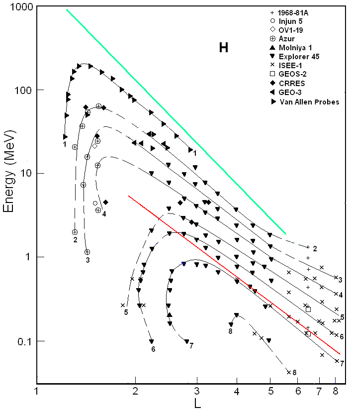
Figure 2 Proton fluxes in the ERB near maxima of the solar activity. The numbers on the curves refer to the values of the decimal logarithms of J, which are given in units of ions per square centimeter per second per steradian per Mev/nucleon (cm² s sr MeV)⁻¹, and are the differential fluxes of protons with ${\mathit{\alpha }}_{\mathrm{0}}\approx {\mathrm{90}}^{\circ }$ (near the plane of the geomagnetic equator). Data from satellites are associated with different symbols (see legend). The red line corresponds to the lower boundary of the power-law tail of the proton spectra, and the green line corresponds to the maximum energy of protons trapped in the ERB (Ilyin et al., 1984).

The red line corresponds to the lower boundary (E_b) of the power-law tail of the proton spectra. For this line, $E_{\mathrm{b}}\sim \mathrm{36}\times L^{-\mathrm{3}}$ MeV. Some changes in the slope of these isolines at L>6 can be connected to a discrepancy between the real configuration of the magnetic field lines and the dipolar configuration (used here for the L shell's calculation and for the red line).

For the dipole magnetic field region, the points on the red line correspond to particles with a specific value of the first adiabatic invariant of motion (μ_b). For Figs. 1 and 2, the average value μ_b is ∼1.16 keV nT⁻¹. Segments of isolines that are parallel to the red line also correspond to certain values of the invariant μ. In this region of the {E.L} space the ionization and other losses of the ERB protons during radial drift can be neglected, and changes of fluxes with changing L are practically reduced to adiabatic transformations in a magnetic field.

From these figures, it can be noted that the value $\mathit{\gamma }=\mathrm{4.8}\pm \mathrm{0.5}$ at L=3–6. At L>6, the distances between these isolines increase with L, and the value γ is decreased from ∼4.7–5.0 at L=6 to ∼4.1–4.5 at L=8. This is due to the deviation of the magnetic field from the dipole configuration as well as to the increasing variability of this field with increasing L.

According to the data from the satellites considered in Kovtyukh (2001), invariant parameters μ_b and γ were only found at L>3. In this work, a wider range of L and E is considered; for protons with E>10 MeV, these parameters can be traced to L∼2. At L=2, $\mathit{\gamma }=\mathrm{4.4}\pm \mathrm{0.6}$ (Fig. 1) and $\mathit{\gamma }=\mathrm{4.7}\pm \mathrm{1.3}$ (Fig. 2). This is due to the fact that the energy range is significantly extended toward higher values (up to 200 MeV), but the ionization losses for protons rapidly decrease here (see, e.g., Schulz and Lanzerotti, 1974; Kovtyukh, 2016a).

2.2 Spatial-energy structure of the helium ion fluxes

In Figs. 3 and 4, helium ion fluxes, which have been averaged for quiet periods (Kp <2), are presented.

Figure 3 summarizes results from the Molnija 2 (Panasyuk et al., 1977), the Prognoz 5 (Lutsenko and Nikolaeva, 1978), the ISEE-1 (International Sun-Earth Explorer 1; Hovestadt et al., 1981), as well as the Akebono (or EXOS-D – Exospheric Satellite D) and the ETS-VI (Engineering Test Satellite) (Goka et al., 1999) satellites. These results were collected during minimum periods of various solar cycles, i.e., between the 20th/21th (1975–1977), 21th/22th (1984–1985), and 22th/23th (1994–1996) solar activity cycles.

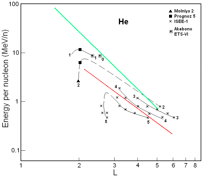
Figure 3 Helium ion fluxes in the ERB near minima of the solar activity. The numbers on the curves refer to the values of the decimal logarithms of J, which are given in units of ions per square centimeter per second per steradian per Mev/nucleon (cm² s sr MeV/n)⁻¹, and are the differential fluxes of helium ions with ${\mathit{\alpha }}_{\mathrm{0}}\approx {\mathrm{90}}^{\circ }$ (near the plane of the geomagnetic equator). Data from satellites are associated with different symbols (see legend). The red line corresponds to the lower boundary of the power-law tail of the helium spectra, and the green line corresponds to the maximum energy of these ions trapped in the ERB (Ilyin et al., 1984).

Figure 4 summarizes results from the OV1-19 (Orbiting Vehicle 1–19; Blake et al., 1973; Fennell and Blake, 1976), the Explorer 45 (Fritz and Spjeldvik, 1978, 1979; Spjeldvik and Fritz, 1981), and the SCATHA (Spacecraft Charging At High Altitudes; Blake and Fennell, 1981; Chenette et al., 1984) satellites. These results were obtained during maximum periods of the 20th (1968–1971) and 21th (1979) solar cycles.

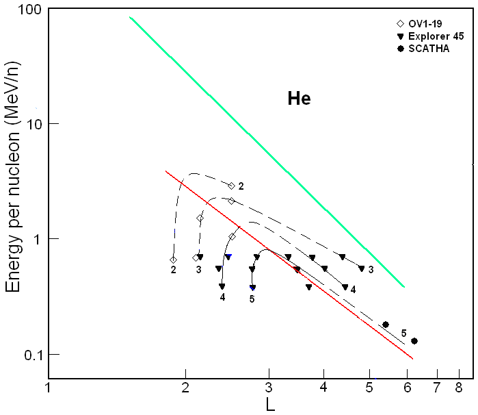
Figure 4 Helium ion fluxes in the ERB near maxima of the solar activity. The numbers on the curves refer to the value of the decimal logarithms of J, which are given in units of ions per square centimeter per second per steradian per Mev/nucleon (cm² s sr MeV/n)⁻¹, and are the differential fluxes of ions with ${\mathit{\alpha }}_{\mathrm{0}}\approx {\mathrm{90}}^{\circ }$ (near the plane of the geomagnetic equator). Data from satellites are associated with different symbols (see legend). The red line corresponds to the lower boundary of the power-law tail of the helium spectra, and the green line corresponds to the maximum energy of these ions trapped in the ERB (Ilyin et al., 1984).

From a comparison of Figs. 1 and 2 with Figs. 3 and 4, one can see that the solar-cyclic (11-year) variations are greater for helium ions than for protons at L>2. For example, at L∼2–3, from the maximum to minimum of solar activity, fluxes of protons with E>1 MeV practically do not change, and the fluxes of helium ions with E>1 MeV/n are increased by 1 order of magnitude.

Figures 3 and 4 show the same patterns as for protons, but the distribution of helium ion fluxes is slightly shifted towards higher values of the L shell (with respect to protons). Unlike protons, there are significant “white spots” in these figures, as there are no experimental data for helium ions in these regions.

The red line on these figures corresponds to the lower boundary of the power-law tail of the helium ion spectra. For this line, $E_{\mathrm{b}}/M_{\mathrm{i}}\sim \mathrm{43.4}\times L^{-\mathrm{3}}$ MeV/n (Fig. 3) and $E_{\mathrm{b}}/M_{\mathrm{i}}\sim \mathrm{21.7}\times L^{-\mathrm{3}}$ MeV/n (Fig. 4). If one takes into account that the average charge $Q_{\mathrm{i}}=+\mathrm{2}$ for helium ions with E>0.2 MeV/n at L<6 (see, e.g, Spjeldvik, 1979), we get ${\mathit{\mu }}_{\mathrm{b}}\sim \mathrm{1.4}\times Q_{\mathrm{i}}$ keV nT⁻¹ for the boundary considered at the maximum of solar activity and ${\mathit{\mu }}_{\mathrm{b}}\sim \mathrm{1.4}\times M_{\mathrm{i}}$ keV nT⁻¹ at the minimum of solar activity (for the dipole magnetic field region). The isolines of helium ion fluxes in Figs. 3 and 4, which pass above the red line at L>2.5, correspond to an average value of γ∼5.5 (there is a large uncertainty due to the small energy range covered).

For helium spectra, as for proton spectra, the values of the parameters of the power-law tail are in agreement with what was found in Kovtyukh (2001).

At the same time, one can see that the isolines of the fluxes of helium ions in the region above the red line (i.e., in the region of power-law spectra) substantially deviate from the slope of the red line. At L>3, the fluxes of helium ions with a given energy increase with decreasing L more slowly than is the case for protons. This means that the ionization losses of the ERB helium ions significantly exceed the losses for protons, which is in agreement with well-known calculations (see, e.g., Schulz and Lanzerotti, 1974). For example, the Coulomb loss rate increases with increasing Z of the ions as Z².

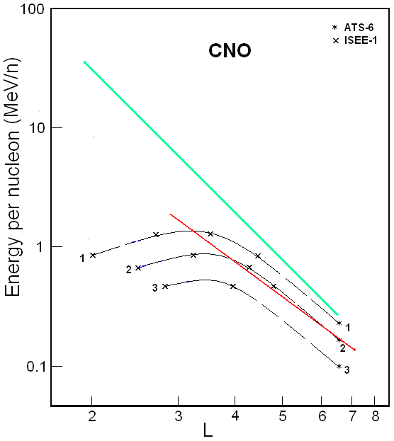
Figure 5 CNO ion fluxes in the ERB near minima of the solar activity. The numbers on the curves refer to the values of the decimal logarithms of J, which are given in units of ions per square centimeter per second per steradian per Mev/nucleon (cm² s sr MeV/n)⁻¹, and are the differential fluxes of ions with ${\mathit{\alpha }}_{\mathrm{0}}\approx {\mathrm{90}}^{\circ }$ (near the plane of the geomagnetic equator). Data from satellites are associated with different symbols (see legend). The red line corresponds to the lower boundary of the power-law tail of the CNO ion spectra, and the green line corresponds to the maximum energy of these ions trapped in the ERB (Ilyin et al., 1984).

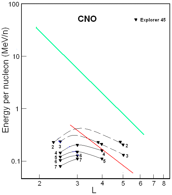
Figure 6 CNO ion fluxes in the ERB near the maximum of the solar activity. The numbers on the curves refer to the values of the decimal logarithms of J, which are given in units of ions per square centimeter per second per steradian per Mev/nucleon (cm² s sr MeV/n)⁻¹, and are the differential fluxes of ions with ${\mathit{\alpha }}_{\mathrm{0}}\approx {\mathrm{90}}^{\circ }$ (near the plane of the geomagnetic equator). Data from satellites are associated with different symbols (see legend). The red line corresponds to the lower boundary of the power-law tail of the CNO ion spectra, and the green line corresponds to the maximum energy of these ions trapped in the ERB (Ilyin et al., 1984).

2.3 Spatial-energy structure of the CNO group ion fluxes

In Figs. 5 and 6 CNO group ion fluxes, averaged for quiet periods (Kp <2), are presented.

Figure 5 summarizes results from the ATS-6 (Applications Technology Satellite 6; Spjeldvik and Fritz, 1978; Fritz and Spjeldvik, 1981) and the ISEE-1 (International Sun-Earth Explorer 1; Hovestadt et al., 1978) satellites. These results were collected during a minimum period between the 20th/21th solar activity cycles (1974–1975, 1977).

Figure 6 summarizes results from the Explorer 45 (Spjeldvik and Fritz, 1978; Fritz and Spjeldvik, 1981) satellite. These results were obtained during a maximum period of activity in the 20th solar cycle (1971–1972).

In Figs. 5 and 6 the spatial-energy patterns of the ion fluxes of the CNO group are even more shifted towards higher values of the L shell, and its configuration differs significantly from Figs. 1–4.

From a comparison of Figs. 1 and 2 with Figs. 5 and 6, one can see that the solar-cyclic (11-year) variations are greater for ions of the CNO group than for protons. For example, at L∼3–5, from the maximum to minimum of solar activity, fluxes of protons with E>1 MeV practically do not change, but the fluxes of the CNO group increase by 1 order of magnitude or more. From a comparison of Figs. 3 and 4 with Figs. 5 and 6, it is also seen that the fluxes of the CNO group change several times more than the fluxes of helium ions do. For ions of the CNO group, this means that the ionization losses at L=3–5 are much larger than for ions with Z≤2, and these losses even have a significant effect on the power-law segment of the spectra of the CNO ions (in the part that is seen on Figs. 5 and 6). Therefore, the lower boundary of the power-law tail of these ions' spectra was not obtained by the experiments collected in Figs. 5 and 6. The red line on these figures corresponds to adiabatic laws (see Kovtyukh, 2001); this line allows us to estimate the deviations from these laws. As can be seen from Figs. 5 and 6, ionization losses for ions of the CNO group are especially large at the peak of solar activity (Fig. 6): during these times, the slope of isolines on L>3 is significantly less than the slope of the red line.

At the same time, at L>4 in Fig. 5 and at L>3 in Fig. 6, the isolines of fluxes pass almost parallel to each other and at approximately equal distances from each other; the average value of γ corresponding to them is ∼6 (there is a large uncertainty due to the small energy range covered). Thus, for sufficiently large values of E and L, the CNO group ions' spectra in the ERB have a power-law form, but these spectra are softer in comparison with the spectra of protons. Here, the red line corresponds to the dependences $E_{\mathrm{b}}/M_{\mathrm{i}}\approx \mathrm{43.4}\times L^{-\mathrm{3}}$ MeV/n (in Fig. 5) and $E_{\mathrm{b}}/M_{\mathrm{i}}\sim \mathrm{12.4}\times L^{-\mathrm{3}}$ MeV/n (in Fig. 6) that are taken from Kovtyukh (2001), where this boundary was also more clearly defined for the ions of the CNO group. If one takes into account that the average charge $Q_{\mathrm{i}}=+\mathrm{4}$ for the CNO group ions with E>0.1 MeV/n at L∼3–5 (see, e.g., Spjeldvik and Fritz, 1978), one can obtain ${\mathit{\mu }}_{\mathrm{b}}\sim \mathrm{1.4}\times Q_{\mathrm{i}}$ keV nT⁻¹ for this boundary at the maximum of solar activity and ${\mathit{\mu }}_{\mathrm{b}}\sim \mathrm{1.4}\times M_{\mathrm{i}}$ keV nT⁻¹ at the minimum of solar activity (for the dipole magnetic field region).

3 Discussion

Let us consider the conclusions following the results obtained here for solar-cyclic variations in the fluxes of ERB ions. Solar-cyclic (11-year) variations of proton fluxes with E>1 MeV in the inner region of the ERB have been studied in many works (see, e.g., Pizzella et al., 1962; Hess, 1962; Blanchard and Hess, 1964; Filz, 1967; Nakano and Heckman, 1968; Vernov, 1969; Dragt, 1971; Huston et al., 1996; Vacaresse et al., 1999; Kuznetsov et al., 2010; Qin et al., 2014). These variations reach 1 order of magnitude at L=1.14 and are rapidly reduced with increasing L (see, e.g., Vacaresse et al., 1999). However, solar-cyclic variations of fluxes of ions with Z≥2 have not been considered in these works.

In these studies, such variations of the proton fluxes of the inner belt are connected to the solar-cyclic variations of the energy loss rates of protons in this region. For protons with E>10 MeV of the inner ERB, the effect of attenuation of GCR proton fluxes in the Earth's orbit with increasing solar activity acts in the same direction (see, e.g., Usoskin et al., 2005; Selesnick et al., 2007). We must also take secular variations of the geomagnetic dipole moment into account (see, e.g., Selesnick et al., 2007).

Consider the solar-cyclic variations of the ERB ion fluxes in connection with variations of the energy loss rates of these ions in more detail. In quiet periods, only the mechanism of ionization loss is significant for the ERB protons trapped in small L shells (see, e.g., Schulz and Lanzerotti, 1974). In this mechanism, energy loss rates and lifetimes of the ERB protons are determined by the density of atmospheric atoms and ionospheric plasma (N) in a geomagnetic trap. This density depends on the intensity of the ultraviolet radiation of the Sun. With decreasing solar activity (with a transition from maximum to minimum of the solar cycle), the densities of atmospheric atoms and ionospheric plasma in a geomagnetic trap decrease and, therefore, the stationary proton fluxes increase with decreasing solar activity.

The lifetimes of protons increase with L; this leads to a decrease in the amplitude of the solar-cyclic variations of proton fluxes. A proton lifetime on a given L shell depends on its energy and is less than 11 years ($\sim \mathrm{3.5}\times {\mathrm{10}}^{\mathrm{8}}$ s) at L<L_c(E). For example, for protons with E>6 MeV, the value L_c is ∼2.5 and corresponds to protons with μ>3 keV nT⁻¹ (see, e.g., Kovtyukh, 2016b, Fig. 3). Figures 1 and 2 show that the solar-cyclic variations of fluxes are small and localized at L<2.5 (mainly at L<1.4) for protons.

In contrast to protons, Figs. 3–6 show significant solar-cyclic variations of fluxes of helium ions and CNO group ions at L∼2–5. There is low density of atmospheric atoms and ionospheric plasma in that region (compared with L<2), but the density changes consistently with solar cycle.

For ions with Z≥2 in the ERB, ionization losses are more significant than for protons, and this can be connected to the absence of ions with Z≥2 at L<2 (or very low values of these fluxes) during quiet geomagnetic conditions. Such short lifetimes are also manifested in the slope of the experimental curves in Figs. 4 and 6 (this was noted in Sect. 2.2 and 2.3, respectively). Consequently, for ions with Z≥2, the regions in which variations can manifest, should be located on higher L shells (at the same energies as for protons).

The lifetimes of ions in the energy ranges considered here are $\mathit{\tau }\propto M_{\mathrm{i}}^{-\mathrm{1}/\mathrm{2}}{Q}_{\mathrm{i}}^{-\mathrm{2}}{N}^{-\mathrm{1}}{E}^{\mathrm{3}/\mathrm{2}}$ (Schulz and Lanzerotti, 1974). In a first approximation, for $N\propto L^{-\mathrm{4}}$, we obtain the value $L_{\mathrm{ci}}\sim M_{\mathrm{i}}^{\mathrm{1}/\mathrm{8}}{Q}_{\mathrm{i}}^{\mathrm{1}/\mathrm{2}}{L}_{\mathrm{c}}$, where L_c corresponds to the L shell of protons of the same energy as the other ions under study. For helium ions (M_i=4, Q_i=2) with E∼6 MeV, we obtain outer boundary L_ci∼4.2. For ions of the CNO group (M_i=14, Q_i=4) with E∼6 MeV, we obtain outer boundary L_ci∼6.9. These are very rough estimations, but they are in agreement with the results presented in Figs. 3–6.

These estimates are based on the following assumption: during variations in solar activity, the rates of ion supply on L<L_ci remains unchanged (or these changes are weaker than the effect of changes of the rate of ion losses). The stationary ion fluxes of the ERB at L>2.5 form mainly under the action of radial diffusion (see, e.g., Schulz and Lanzerotti, 1974; Kovtyukh, 2016b, 2018). Therefore, the solar-cyclic variations of Z≥2 ion fluxes can be motivated only under the assumption that the effect related to an increase in the ionization losses of such ions significantly exceeds the effect connected with the possible enhancement of radial diffusion of ions during the rising phase of solar activity. For example, when comparing the empirical model of the inner belt (L<2.4) of protons with E∼19–200 MeV, constructed on the data from Van Allen Probes, with the mathematical model of radial diffusion of protons in this region, it was assumed that D_LL increases by only ∼2 times on the phase of growth of solar activity from 2013 to 2015 (Selesnick and Albert, 2019).

In the experimental results presented here for the ERB ions, the region of the power-law tail of the ion spectra is distinguished. For many experiments, especially for heavy ions, the values of the parameter of a power-law tail spectra are determined much more accurately by the dependences J(L) of the ion fluxes (on a logarithmic scale) for different pairs of energy channels (see Kovtyukh, 2001). For example, the range of L in which these dependences for two energy channels are parallel to each other is connected to the power-law tail of the spectra. In contrast, for smaller values of L, these fluxes begin to converge, and the radial dependences of these fluxes intersect with each other, which is related to the maximum in the spectra.

The main source of ions in the outer regions of the ERB is the solar wind, and the high-energy part of these spectra usually have an exponential shape (see, e.g., Ipavich et al., 1981a, b). Immediately before being captured into the magnetosphere, these ions pass through a highly turbulized region, but the high-energy part of their spectra usually retains an exponential shape. Therefore, the following question arises: what physical mechanism converts the form of the ion spectra from exponential to power-law?

Evidently, the power-law tail of the ERB ions' spectra must be generated in the outer regions of the magnetosphere. The most likely region for this to happen is the plasma sheet (PS) of the magnetospheric tail, which is adjacent to the geomagnetic trap. The high-energy part of the ion spectra in the PS, at R∼20–40 R_E, has a power-law shape, and the exponents of these spectra are close to the corresponding parameters of the spectra of ions in the ERB. Based on the data from the IMP 7 and IMP 8 satellites (Sarris et al., 1981; Lui and Krimigis, 1981) as well as the ISEE-1 (Christon et al., 1991) satellite, the shape of the ion spectra of the PS usually do not change during substorms; they only produce parallel shifts of the spectra along the logarithmic axes E and J. These results point out that the timescales of the formation processes of these ion spectra in the PS exceed the time spans of substorms.

Parameters of the power-law tail of the ion spectra of the outer belt (γ and μ_b) apparently reflect the most fundamental features of the mechanisms of the acceleration of ions in the tail of the magnetosphere. One can try to connect the values of these parameters with the most general representations of the mechanisms of ion acceleration in the PS of the magnetospheric tail.

Most likely, this part of the ion energy spectra is formed in the PS by stochastic mechanisms of ion acceleration; this hypothesis is supported by many experimental results. The statistical aspect of these mechanisms reveals itself, in particular, in the fact that the ratios of fluxes (and partial densities) of ions with different Z can differ (even greatly) at low and high energies. During their wander in the phase space, ions gradually lose information about their origin; therefore, the high-energy tails of their spectra contain ambiguous information on the partial densities of different components of ions in the source (see, e.g., Kovtyukh, 2001).

The high-energy part of the ion spectra of the PS can be generated by the mechanisms of the acceleration of particles on magnetic irregularities moving with respect to each other (the Fermi mechanism). The fractal structures of the PS are revealed on scales from ∼0.4 to ∼8000 km, for example, in the data from the Geotail satellite (Milovanov et al., 1996).

Under equilibrium conditions, this parameter is determined by the average part of energetic ions in the total energy density of particles and magnetic irregularities ($\overline{\mathit{\beta }}$). From the theory, which was developed by Ginzburg and Syrovatskii (1964), it follows that $\mathit{\gamma }-\mathrm{1}\approx (\mathrm{1}-\overline{\mathit{\beta }}{)}^{-\mathrm{1}}$. With increasing $\overline{\mathit{\beta }}$ in the interval $\mathrm{0}<\overline{\mathit{\beta }}<\mathrm{1}$, the value γ increases monotonically and γ→∞ for $\overline{\mathit{\beta }}\to \mathrm{1}$. For real average values, $\overline{\mathit{\beta }}$ in the central PS $\overline{\mathit{\beta }}=\mathrm{0.6}$–0.7 (see, e.g., Baumjohann, 1993, Fig. 1), we get γ=3.5–4.3.

Spectra with a power-law tail and quasi-exponential segment at lower energies can be generated when the value $\mathrm{\Delta }B/\overline{B}$ for magnetic irregularities is proportional to their size δr and their spectral density decreases rapidly with increasing δr for δr<r_s (r_s is a thickness of the central PS), but for δr>r_s it remains almost unchanged. Apparently, the spectra of magnetic irregularities in the PS have just such a form (see, e.g., Milovanov et al., 1996). Then, the lower boundary μ_b of the power-law tail corresponds to the condition r_s/ρ_i∼10, where ρ_i is the gyroradius of ions (see, e.g., Alfvén and Fälthammar, 1963), i.e., ${\mathit{\mu }}_{\mathrm{b}}\sim \mathrm{0.02}(Q_{\mathrm{i}}^{\mathrm{2}}/M_{\mathrm{i}})B_{\mathrm{s}}{r}_{\mathrm{s}}^{\mathrm{2}}$ keV nT⁻¹, where B_s is the average magnetic field induction in the PS (in nT) and r_s is normalized to the Earth's radius. Using B_s∼30 nT and r_s∼1.3R_E (see, e.g., Baumjohann, 1993), the following can be obtained: ${\mathit{\mu }}_{\mathrm{b}}\sim \mathrm{1.0}(Q_{\mathrm{i}}^{\mathrm{2}}/M_{\mathrm{i}})$ keV nT⁻¹. This value is similar to the lower boundary of the power-law spectrum which we find for the ERB protons, suggesting that not only the slope of the spectrum but also its validity range can be explained by scattering at magnetic irregularities.

The energy spectra of ions in the radiation belts of planets such as Jupiter and Saturn have a form analogous to that of ion spectra in the ERB (see, e.g., Krimigis et al., 1981; Cheng et al., 1985; Kollmann et al., 2011). As seen in the ERB, these spectra have a long power-law tail, which is apparently formed by mechanisms of the stochastic acceleration of ions as a result of their interactions with the current layer of the magnetospheric tail.

4 Conclusions

In this work, the experimental results for the stationary fluxes of the main ion components of the ERB (protons, helium ions, and ions of the CNO group) in the near-equatorial plane, were analyzed. It was been found that these fluxes line up in the certain regular patterns in the {E,L} space in the outer belt . The degree of similarity increases with increasing E and L, and it is linked to the nature of the main sources and to the universality mechanisms of transfer, acceleration, and losses of ERB ions in the outer belt (radial diffusion which conserves μ and K of ions, betatron acceleration, and ionization losses). Moreover, solar-cyclic (11-year) variations of the spatial-energy distributions of the ERB ion fluxes were investigated. It was noted that the ERB ion fluxes are weaker with increasing solar activity and this effect increases with increasing atomic number Z. This kind of dependence of the amplitude of flux changes on Z is also typical for faster variations in the fluxes of the ERB ions, during geomagnetic storms, and during other disturbances of the Earth's magnetosphere, as has been underlined in the review by Kovtyukh (2018).

The figures presented here make it possible to determine the regions of the {E,L} space near the equatorial plane in which the ionization losses of ions during their radial diffusion can be neglected and where they cannot. These results also indicate that the coefficient D_LL of the radial diffusion of the ERB ions changes much less than the ionization losses rates of ions with Z≥2 due to variations in the level of solar activity.

In addition, the figures given here reveal the localization of “white spots”, which are especially extensive for ions with Z≥2 and E>1 MeV/n at L<3. As Z and energy become larger and L becomes smaller, the uncertainties in the values of the ERB fluxes become larger. These gaps must be filled by the results of future experiments on satellites; for now, the extensive gaps in Z≥2 ion data do not allow for the creation of sufficiently complete and reliable empirical models of the ERB for these ions.