High-latitude crochet: solar-flare-induced magnetic disturbance independent from low-latitude crochet

A solar-flare-induced, high-latitude (peak at 70–75^∘ geographic latitude – GGlat) ionospheric current system was studied. Right after the X9.3 flare on 6 September 2017, magnetic stations at 68–77^∘ GGlat near local noon detected northward geomagnetic deviations (ΔB) for more than 3 h, with peak amplitudes of >200 nT without any accompanying substorm activities. From its location, this solar flare effect, or crochet, is different from previously studied ones, namely, the subsolar crochet (seen at lower latitudes), auroral crochet (pre-requires auroral electrojet in sunlight), or cusp crochet (seen only in the cusp). The new crochet is much more intense and longer in duration than the subsolar crochet. The long duration matches with the period of high solar X-ray flux (more than M3-class flare level). Unlike the cusp crochet, the interplanetary magnetic field (IMF) B_Y is not the driver, with the B_Y values of only 0–1 nT out of a 3 nT total field. The equivalent ionospheric current flows eastward in a limited latitude range but extended at least 8 h in local time (LT), forming a zonal current region equatorward of the polar cap on the geomagnetic closed region.

EISCAT radar measurements, which were conducted over the same region as the most intense ΔB, show enhancements of electron density (and hence of ion-neutral density ratio) at these altitudes (∼100 km) at which strong background ion convection (>100 m s⁻¹) pre-existed in the direction of tidal-driven diurnal solar quiet (Sq0) flow. Therefore, this new zonal current can be related to this Sq0-like convection and the electron density enhancement, for example, by descending the E-region height. However, we have not found why the new crochet is found in a limited latitudinal range, and therefore, the mechanism is still unclear compared to the subsolar crochet that is maintained by a transient redistribution of the electron density.

The signature is sometimes seen in the auroral electrojet (AE = AU − AL) index. A quick survey for X-class flares during solar cycle 23 and 24 shows clear increases in AU for about half the > X2 flares during non-substorm time, despite the unfavourable latitudinal coverage of the AE stations for detecting this new crochet. Although some of these AU increases could be the auroral crochet signature, the high-latitude crochet can be a rather common feature for X flares.

1. We found a new type of the solar flare effect on the dayside ionospheric current at high latitudes but equatorward of the cusp during quiet periods.

2. The effect is also seen in the AU index for nearly half of the > X2-class solar flares.

3. A case study suggests that the new crochet is related to the Sq0 (tidal-driven part) current.

1 Introduction

Solar flares are known to enhance the ionospheric electron density and, thus, influence the electric currents in the D- and E-region. The geomagnetic disturbance (ΔH, ΔD, and ΔZ) caused by this current system is called a crochet (e.g. Dodson and Hedeman, 1958) or solar flare effect (SFE; e.g. Curto et al., 1994). Crochets are observed in the following three regions: dayside low latitudes, with a peak near the subsolar region (Curto et al., 1994); in the nightside high-latitude auroral region, with a peak where the geomagnetic disturbance ΔB pre-exists during solar illumination (Pudovkin and Sergeev, 1977); in the cusp (Sergeev, 1977). This paper distinguishes them by calling them the subsolar crochet, auroral crochet, and cusp crochet, respectively.

The subsolar crochet is most likely caused by a redistribution of the electron density at a <120 km altitude that is enhanced by the flare X-ray (e.g. Curto et al., 1994; Yamasaki and Maute, 2017), resulting in a twin vortex (one in each hemisphere) ionospheric current that is similar to the tidal-driven (daily neutral convection starting from subsolar region) part of solar quiet (Sq) ionospheric current, Sq0, which dominates the low-latitude (low solar zenith angle) diurnal convection. All recent studies of the crochet (all three types are equally called crochet, without distinction) refer to this type of disturbance. Sq also has a high-latitude part, SqP, that is driven by the solar wind-magnetosphere coupling for lowest coupling (quiet) condition, giving a different current direction from Sq0 ionospheric current (Matsushita, 1971). However, SqP is found only at high geomagnetic latitudes and is not relevant to the subsolar crochet.

The auroral crochet is most likely caused by the modification of a pre-existing ionospheric current (or electrojet) by the enhanced electron density (Pudovkin, 1974). This effect increases as background plasma convection (ionospheric electric field) increases and, hence, is most visible during the polar disturbances of DP1 and DP2 (Akasofu, 1964; Nishida, 1968), as long as the ionosphere is sunlit, for example, near summer solstice when X-ray flux reaches high latitudes.

The preference of strong background plasma convection applies even to ΔB in the cusp that is strongly controlled by the interplanetary magnetic field (IMF) B_Y (DPY; Friis-Christensen and Wilhjelm, 1975; Levitin et al., 1982). DPY is associated with a narrow “convection throat” which is deflected eastward or westward, depending on the IMF B_Y polarity (Heelis et al., 1976; Yamauchi and Slapak, 2018); hence, solar-flare-induced ΔB at the cusp is expected to show strong IMF B_Y dependence during quiet periods. In fact, Sergeev (1977) showed one case each for both IMF polarities, showing that ΔB at >80^∘ latitude are in the same direction as the IMF B_Y-dependent geomagnetic disturbances. This is the reason for calling this type of crochet the cusp crochet. Since the cusp crochet is localised at the cusp, the SqP that is seen in a wider area has not been considered as important for the cusp crochet.

The amplitude and duration of the subsolar crochet is tens of nanotesla and less than 30 min (mean 16–20 min) no matter how long the high X-ray flux continues (Sergeev, 1977; Curto et al., 1994). Even after the X9.3 flare on 6 September 2017, ΔB was only about 70 nT, and it ended in less than 20 min (Curto et al., 2018) although the X-ray flux exceeded the X-flare level for nearly 2 h (12:00–13:40 universal time – UT), as shown in Fig. 1a. Thus, the subsolar crochet is a transient event that corresponds to the change in the global distribution of electron density after the solar flare, but it is not maintained by high radiation flux.

The relevant ionospheric current is expected to be limited to low and mid-latitudes in the dayside, and the observed subsolar crochet amplitude actually diminishes towards terminator and high latitudes. Therefore, the subsolar crochet near the terminator has simply been assumed to be negligible as it is driven by the weak return current of the crochet current (e.g. Annadurai et al., 2018). With the resultant day–night asymmetric nature, the subsolar crochet can be detected as a short-lived (15–20 min) spike in the mid-latitude geomagnetic indices representing day-night asymmetric disturbances – ASY-H and ASY-D (Singh et al., 2012), whereas the deviation is barely seen in the high-latitude indices (e.g. AU and AL), except near the summer solstice (Sergeev, 1977).

Compared to the subsolar crochet, crochets at high latitudes, including the auroral crochet, have not been studied much for 40 years. This is partly because crochets at high latitudes during quiet periods were considered as being a simple extension of the subsolar crochets towards the summer solstice, and partly because the purpose of the high-latitude crochet studies in the 1970s was to understand the ionospheric electric field during disturbed periods. Such derivation requires many assumptions (Pudovkin and Sergeev, 1977). Since the 1980s, more direct methods (satellite and radar measurements) than using geomagnetic signatures took over for the E-field studies, which led to low research activity on crochets at high latitudes, even during quiet periods.

However, as shown in this paper, we found that the crochet at high latitudes is not a simple extension or sub-effect of, but is independent from, the subsolar crochet with a larger amplitude and longer duration. We show this from a case study of the X9.3 flare on 6 September 2017, using high-latitude magnetometer data in the dayside and EISCAT radar data. We also show how these effects are seen in geomagnetic AE index, using about 60 non-substorm time flares of > X2 class during the past two solar cycles (cycle 23 and 24). The solar flare X-ray data observed by GOES satellites are obtained from NOAA, and the geomagnetic indices are obtained from the World Data Center for Geomagnetism (Kyoto and Copenhagen). The solar wind data and energetic particle data are not shown here because they are not essential to this paper, and they are described in Yamauchi et al. (2018).

2 High-latitude crochet for X9.3 flare on 6 September 2017

In the overview paper of the EISCAT radar observations and geomagnetic disturbances near local noon during the 6–8 September 2017 space weather event, Yamauchi et al. (2018) briefly mentioned a sudden enhancement of ΔB (>150 nT) at high latitudes (>68^∘ GGlat), in response to the X9.3 flare on 6 September 2017, but without a special note or detailed description of this high-latitude disturbance compared to subsolar crochets, auroral crochets, or cusp crochets.

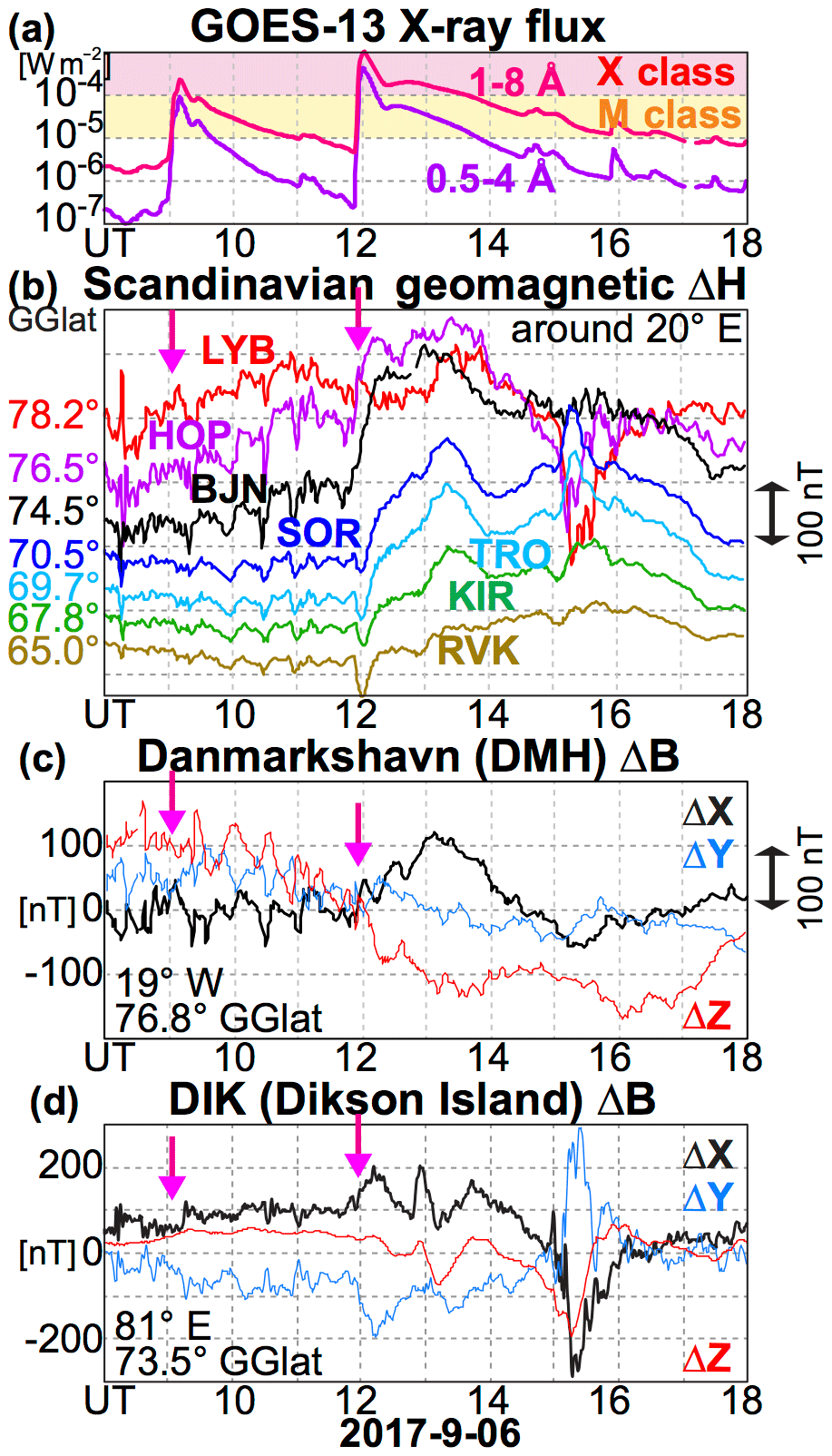
Figure 1 (a) Solar X-ray flux. (b) Stack plot of the geomagnetic D component for Kiruna (KIR) and northern Norway. (c) Geomagnetic data at Danmarkshavn (DMH) and (d) at Dikson Island (DIK).

2.1 Subsolar crochet after X9.3 flare

Figure 1b shows detailed time profiles of the northern Scandinavian magnetograms at >65^∘ GGlat, which are located near local noon when the X9.3 flare took place. Although the Fig. 1 period is in the middle of the space weather event that started on 4 September 2017, the magnetic storm did not start until the end of 6 September. Furthermore, the solar wind during this period was stable, at around 450 km s⁻¹ (slightly declining in time), and IMF was weak, with a total field less than 3 nT ($B_X=-\mathrm{1}$ nT, B_Y=1 to 0 nT, $B_Z=-\mathrm{2}$ nT during 12:00–13:00 UT in the geocentric solar magnetospheric (GSM) coordinate), as shown in Yamauchi et al. (2018; Fig. 1). Such a stable condition caused the preceding substorm activity before the X9.3 flare to diminish before the flare onset, as seen in the geomagnetic indices (Fig. 2). The IMF B_Y condition indicates that the cusp crochet must be small or invisible.

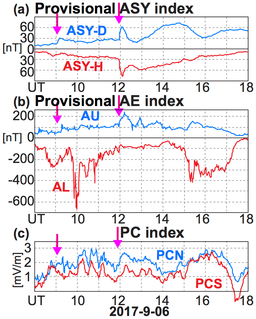
Figure 2 Geomagnetic indices that represent asymmetric disturbances at midlatitude (ASY), auroral electrojet (AE), and polar cap electric field (PC).

The subsolar crochet was observed as being short-lived geomagnetic deviations starting nearly simultaneously as the X-ray flux increased at the Earth and lasted about 10–15 min at Sørøya (SOR; 70.5^∘ GGlat), Tromsø (TRO; 69.7^∘ GGlat), Kiruna (KIR; 67.8^∘ GGlat), and Rørvik (RVK; 65.0^∘ GGlat.). All equatorward stations show the same type of disturbances (Curto et al., 2018). This is also seen in ASY-D (63 nT at 12:04 UT) and ASY-H (77 nT at 12:05 UT), as shown in Fig. 2a, with an amplitude change by the flare of about 60 nT. One can even recognise a crochet-like signature in ASY-D when an X2.2 flare occurred at around 09:00 UT.

2.2 New crochet after X9.3 flare

The new finding is the subsequent geomagnetic disturbances; a large positive ΔH deviation (northward ΔB) also started right after or even during the negative ΔH spike (southwestward ΔB) of the subsolar crochet, with much higher amplitudes, as shown in Fig. 1b. This positive ΔH continued for hours, with the peak at around 13:00 UT at Bear Island (BJN) at 74.5^∘ GGlat (>200 nT), 13:20 UT at 70^∘ GGlat (SOR and TRO – 180 nT) and 68^∘ GGlat (KIR – 140 nT), and 14:50 UT at 65^∘ GGlat (ROR – 70 nT). With a larger amplitude and longer duration than the subsolar crochet, this geomagnetic signature is visible even in AU, as shown in Fig. 2b, although the baseline is as large as 100 nT due to the previous substorm activity, and it can hide the subsolar crochet if any exists.

The development is also quick. At BJN (74.5^∘ GGlat), ΔH reached ΔH>65 nT at 12:05 UT already, i.e. at the peak time of the subsolar crochet, and reached 130 nT at 12:20 UT. Since the long duration already indicates that the generation mechanism is different from that of the subsolar crochet (redistribution of electron), the positive ΔH of this crochet with diminishing amplitude towards lower latitudes should cancel the negative ΔH of the subsolar crochet at high latitudes. In fact, ΔH exceeded the value before the flare at 12:10 UT at 70^∘ GGlat, 12:12 UT at 68^∘ GGlat, and 12:17 UT at 65^∘ GGlat.

These large ΔH, however, are observed in a limited latitudinal range, diminishing towards higher latitudes with 140 nT at 76.5^∘ GGlat (Hopen – HOP; 12:50 UT) and not visible at 78.2^∘ GGlat (Longyearbyn – LYB). Since the geomagnetic latitude of LYB is only 75.3^∘, and IMF is weak with B_Y=0 nT, the positive ΔH is limited to the geomagnetic closed region outside the cusp or polar cap. The closed geometry is also indicated by the EISCAT Svalbard radar data (Yamauchi et al., 2018). The polar cap (PC) index, which corresponds to the polar cap activity, shows enhanced values in the same period but not as prominently as in AU, as shown in Fig. 2.

On the other hand, positive ΔB at around 75^∘ GGlat was observed in a wide local time range, as shown in Fig. 1c and 1d (ΔX is nearly the same as ΔH in both stations). Danmarkshavn (DMH; 19^∘ W) and Dikson Island (DIK; 81^∘ E) showed ΔX of about 120 nT and 100 nT at around 13:00 UT, respectively, compared to the values before the flare. Together with the zero IMF B_Y condition, the observed large ΔH cannot be a cusp crochet. Considering its location and pre-existing activity, this crochet is neither a subsolar crochet nor an auroral crochet, although some part of the observed ΔH could be affected by the auroral crochet.

For example, DIK is located near the evening terminator (it is still under sunlight near the horizon), and the geomagnetic activity before 12:00 UT indicates some auroral activity. Therefore, the first peak at around 12:20 UT, which is larger than that of BJN or HOP and with more westward ΔB, can be the auroral crochet rather than the extension of the new crochet. However, the second and third peaks are in the same direction (northward ΔB) as ΔB near local noon, and multiple peaks are not expected for an auroral crochet under a smoothly declining X-ray flux. Therefore, the positive ΔX at DIK at around 13:00 and 13:40 UT can be interpreted as being part of the new high-latitude crochet rather than the auroral crochet, although we cannot dismiss the possibility of the auroral crochet.

With such a large amplitude, the crochet is visible even in AU, although the AE stations are not located at favourable GGlat. During 12:00–14:00 UT, AU has three positive peaks (with provisional values of 240 nT at 12:12 UT, 190 nT at 12:55 UT, and 160 nT at 13:43 UT, while further baseline subtraction might be needed). The timing of these peaks corresponds to the subsolar crochet and the high-latitude one at BJN, but the provisional AU value reflects DIK data (DIK is one of the AE stations), as shown in Figs. 1c and 2b. Although the amplitude is larger at BJN than DIK for the second and third peaks, BJN is located far poleward of the AE stations and did not contribute to AU.

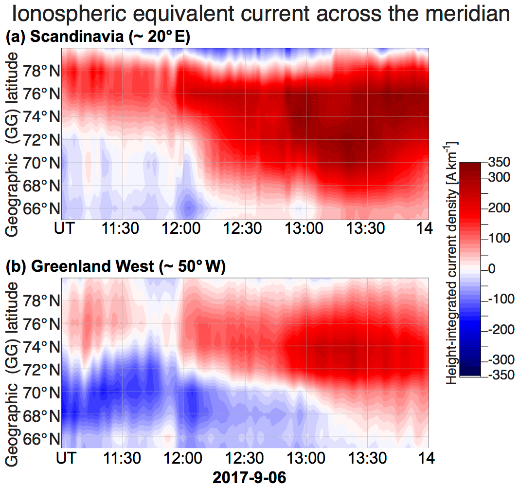
Figure 3 Latitudinal distribution of ionospheric equivalent current (including Sq current) eastward component, (a) crossing Scandinavian meridian (20^∘ E) and (b)  crossing Greenland meridian (50^∘ W), based on the densely distributed magnetometer network. The Spherical Elementary Current System (SECS) technique is used. Data are displayed in a latitude–time spectrogram during 11:00–14:00 UT, 6 September 2017, i.e. around the X9.3 flare.

2.3 Equivalent ionospheric current

From Fennoscandian, Icelandic, and Greenland magnetometer data, we also calculated the ionospheric equivalent currents (including Sq current), using the Spherical Elementary Current System (SECS) technique (Amm, 1998; Amm and Viljanen, 1999). Here, we obtained epsilon = 0.037 in a similar fashion to Wygant et al. (2012). Note that the quiet levels that represent the internal and crustal geomagnetic field (even without Sq) were removed before applying the data to the SECS technique. They were calculated by a least square root approximation (rather than least squares or means), where the square root emphasises the small variations around the quiet level rather than larger disturbances such as substorms. To have a sufficient amount of variations with low activity for the calculation, while avoiding contamination of main field secular variation, the removal of the quiet levels is performed on 10 d of data centred on the day of interest. The uncertainty is estimated to be less than 10 nT (see Edvardsen et al., 2013, for more details).

The results are shown in Figs. 3 and 4. Figure 3 shows the latitudinal distribution of the eastward current density crossing two meridians (Scandinavia – 20^∘ E; Greenland – 50^∘ W) where the actual magnetometer networks are deployed. In Fig. 3, one can see a sudden appearance in the ionospheric current in a wide region at around 12:00 UT when the X-ray flux from the X9.3 flare increased at the Earth. The enhancement is westward at lower latitudes (<70^∘ GGlat at 20^∘ E or 13:00 LT, and <72^∘ W at 50^∘ W or 09:00 LT), and eastward at higher latitudes in both meridians. They correspond to the subsolar crochet current in the northern hemisphere (Curto et al., 2018) and the new high-latitude crochet mentioned above, respectively. Figure 4a and b show the 2D vector directions, corresponding to the timing right before the flare (11:50 UT), and at the peak of subsolar crochet (12:04 UT). The low-latitude side composes the anticlockwise current that agrees with the return current direction of the subsolar crochet at high latitudes (Curto et al., 2018; Annadurai et al., 2018). The high-latitude side forms another independent anticlockwise current, with a strong eastward current near BJN (cf. Fig. 1), as mentioned above. The resultant shear, which is formed poleward of BJN, corresponds to the upward field-aligned current, i.e. to the afternoon Region 1 field-aligned current (Iijima and Potemra, 1976; Yamauchi and Slapak, 2018).

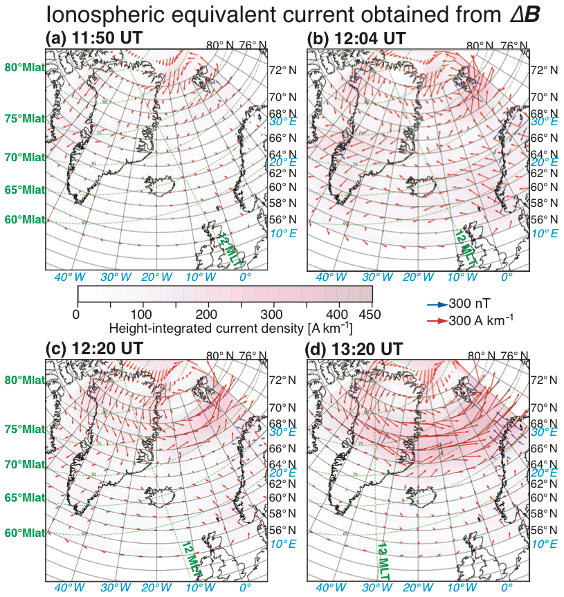
Figure 4 Ionospheric equivalent currents on 6 September 2017, based on magnetometers at Norwegian and Greenland, using the same method as in Fig. 3. (a) Before the flare (11:50 UT), (b) the subsolar crochet peak (12:04 UT), (c) around the first peak at HOP and BJN (12:20 UT), and (d) the main peak at SOR, TRO, and KIR (13:20 UT).

The eastward current expanded quickly in the longitudinal direction and towards lower latitude as soon as the subsolar crochet diminished. At the same time, the current density gradually increased towards its multiple peaks. Figure 4c and d show the 2D vector directions at these peaks; the first minor peak of ΔH (at around 12:20 UT) after the end of the subsolar crochet was located at around 75^∘ GGlat, and the major peak of ΔH (at around 13:20 UT) was located at around 70^∘ GGlat, respectively. By 12:20 UT the area of this westward current that is the most intense at around 72–74^∘ GGlat expanded in a wide local time from Greenland to eventually reach Siberia (DIK at 81^∘ E as shown in Fig. 1d), i.e. more than 130^∘ in longitude. The entire current lies in the geomagnetically closed region, as mentioned above, and its peak latitude gradually moved equatorward. By the peak time at around 13:20 UT, all regions over 5^∘ in latitude and >100^∘ in longitude are intensified, with a much higher intensity than the subsolar crochet current.

The eastward current direction (or positive ΔH) is the same as the ionospheric current in the evening auroral oval (we here mean the region between the upward Region 1 field-aligned current and downward Region 2 field-aligned current; Iijima and Potemra, 1976; Akasofu, 1977; Yamauchi and Slapak, 2018), and the observed eastward current continued until the next substorm onset took place at 15:00 UT (see Fig. 2b). However, no outstanding substorm is visible in AE (Fig. 2b) or DIK data (Fig. 1c) before this substorm with continued weak IMF condition. The eastward current patch even started at the Greenland meridian at 09:00 LT and continued towards the afternoon sector although IMF B_Y=0 nT. Since there was no auroral current signature at BJN before this crochet, this current system is not the auroral crochet current. Rather, the question is how much this new crochet contributes to ΔB in the evening sector, e.g. compared to the auroral crochet. In this sense, we cannot judge for the moment whether the crochet detected in DIK is an evening extension of this crochet or auroral crochet or both effects mixed.

2.4 EISCAT data

For this X9.3 flare event on 6 September 2017, the duration of this new crochet matches with that of the high X-ray flux. It was at the X-class level until 13:40 UT and at the M-class level until about 16:50 UT, as shown in Fig. 1. From this coincidence, Yamauchi et al. (2018) speculated about the possibility of the enhancement of a pre-existing Sq0 (solar quiet tidal-driven) current without showing detailed data. However, the Sq0 has long been expected to be small at high latitudes (Yamasaki and Maute, 2017). Therefore, we need direct evidence with this Sq0 scenario. For that purpose, ionospheric electron density and ion velocity, both observed by EISCAT VHF radar at Tromsø (224 MHz), are shown in Fig. 5.

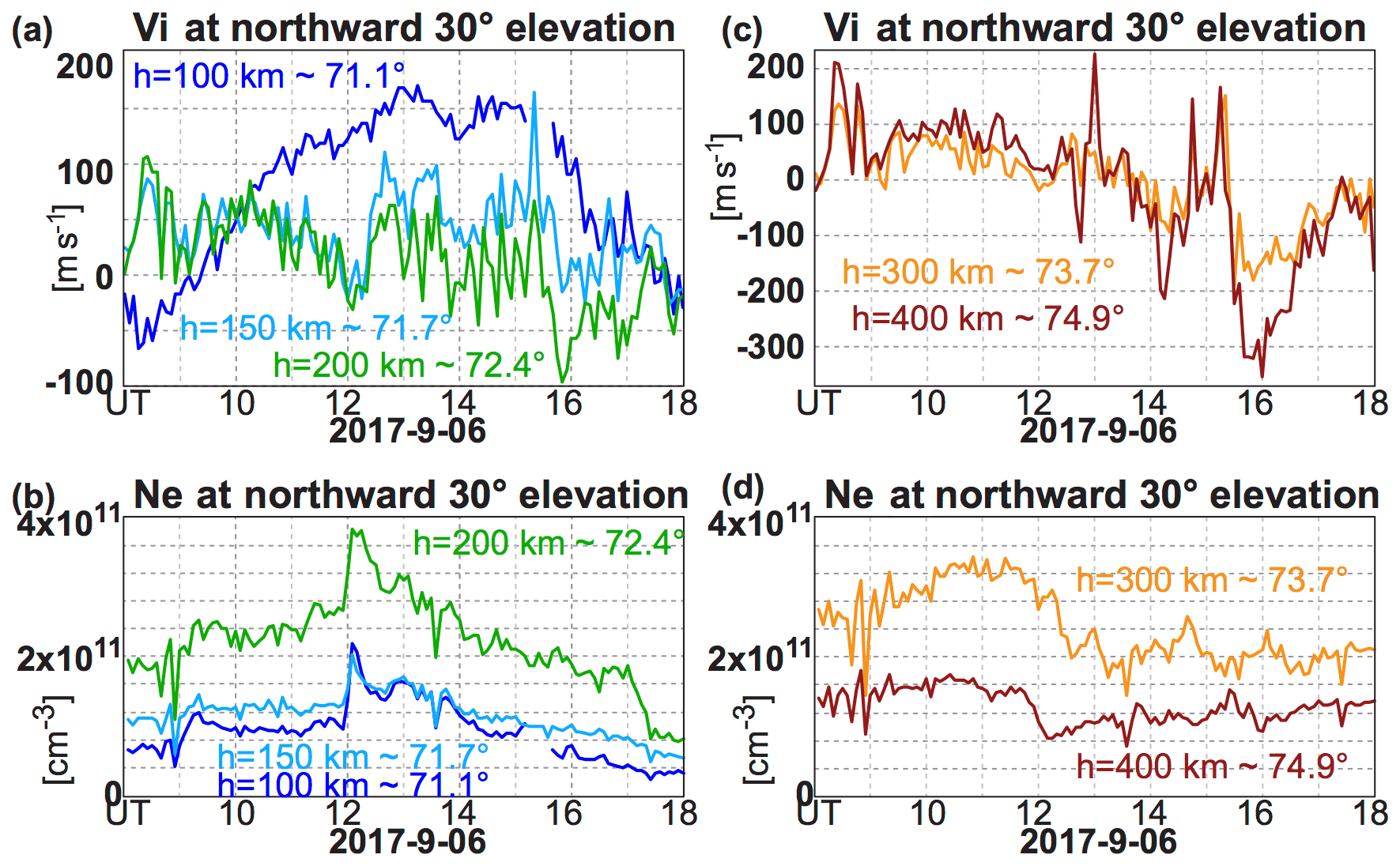
Figure 5 Ionospheric line-of-sight ion velocity and electron density observed by EISCAT Tromsø VHF (224 MHz) radar from 69^∘ GGlat, looking northward at its lowest elevation angle (30^∘) above the horizon. Panels (a) and (c) show the ion velocity, and panels (b) and (d) show the electron density.

Figure 5b shows that the electron densities in the 100–200 km altitude range were significantly enhanced by the enhanced X-ray flux, starting at around 12:00 UT (doubling at 100 km altitude and seen up to 200 km altitude). Figure 5a shows that northward ion convection was also enhanced, and more importantly, that the background Sq0 ion convection (seen as large geomagnetic ΔH>0) starting from around 09:00 UT is already strongly northward (away from the subsolar region), with large values of as much as 150 m s⁻¹ at 71^∘ magnetic latitude (Mlat) at 100 km altitude.

Since the increase in the electron density means an increase in the ion-neutral density ratio too, the ionospheric current is expected to flow at lower altitudes where the tidal (Sq0) ion convection is stronger. Such a change can enhance the pre-existing ionospheric Sq0 current significantly, although this scenario does not easily explain why it is found in a limited latitudinal range and wide longitude.

The time development of the electron density enhancement, together with the elevated ion velocity at 100 km, matches the ΔH time profile at BJN that is located under the area observed by the EISCAT VHF radar. Note that ion velocity direction (northward) is the electric field direction at this altitude, where only ions are collisional with neutrals but not electrons, and hence, collision-free electrons drift westward, resulting in an eastward Hall current (that causes ΔH>0 geomagnetic disturbance).

The EISCAT data in Fig. 5d also revealed a decrease in electron density above 300 km after 12:00 UT. Since photochemistry predicts density increase at all altitudes, this density decrease must be caused by ionospheric dynamics, such as the 3D distribution of ionospheric current. This decrease does not affect the total current because, in addition to the low collision frequency that prevents conduction current, the ion velocity at >300 km did not change very much compared to the ion velocity at <200 km and does not contribute to the ionospheric current.

3 Preliminary survey results

We further conducted a quick survey of the geomagnetic ASY and AE indices during the past two solar cycles. There are 73 flare events with the intensity of > X2 class since 1996. For all these events, we examined the web-interfaced plots of the provisional AE and ASY after adding marks that indicate the X-ray flux level and start timing, as shown in Fig. 6 for 15 July 2002 event. The raw data plots of all 73 events are also found in the Supplement.

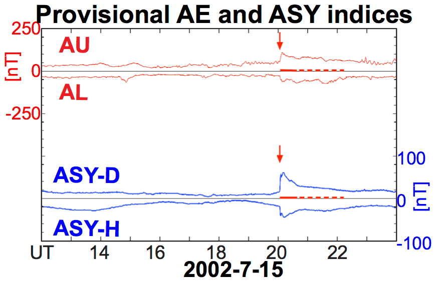
Figure 6 Web-interfaced plots of provisional AE and ASY indices for 15 July 2002. The red horizontal lines correspond to the period when the X-ray flux exceeds $\mathrm{3}\times {\mathrm{10}}^{-\mathrm{5}}$ W m⁻² (> M3 class – solid lines) and 10⁻⁵ W m⁻² (> M class – dashed lines). The vertical red arrow denotes the start of the crochet.

Table 1 shows the survey result. There are about 10 events that occurred during the substorms, and most of the AU and AL variation is too large to determine whether the variation is due to the flare or not, although the crochet is still outstanding in ASY for half of these cases. Among the remaining 63 cases, crochets are almost always detected in ASY, and the exceptions (five cases) might be attributed to a non-favourable distribution of the ASY stations in terms of local time and GGlat at the time of the flare (UT and season). Since auroral crochets and cusp crochets do not contribute to ASY, they are interpreted as subsolar crochets. In addition, crochets are detected in AU and AL for a substantial part of the cases. From the latitude of AE stations, they are either auroral crochet or this new high-latitude crochet.

Table 1 Survey of 73 flare events with the > X2 class.

¹ Simultaneous with the onset. ² Variation (e.g. by substorm) is too large to separate the direct flare effect.

For auroral crochets, the precondition requirement is severe because a substantial auroral electrojet must pre-exist in the sunlit hemisphere. This removes more than half of the cases, and therefore, we expect that the new high-latitude crochet can also be observed in the AE index, as seen in Figs. 3b and  6. In Fig. 6, even AL deviation started simultaneously with the crochet. Then, the question is if this AL signature is related to the crochet or not. In this example, an X3.0 flare started at 19:59 UT, with the X-ray flux reaching M3-class flare level at around 20:05 UT while the solar wind and IMF were stable. AE and ASY show a quiet condition before the flare, and all components (AU, AL, ASY-D, and ASY-H) showed sudden changes at 20:04 UT. The signature is not short-lived; that is typical of the subsolar crochet.

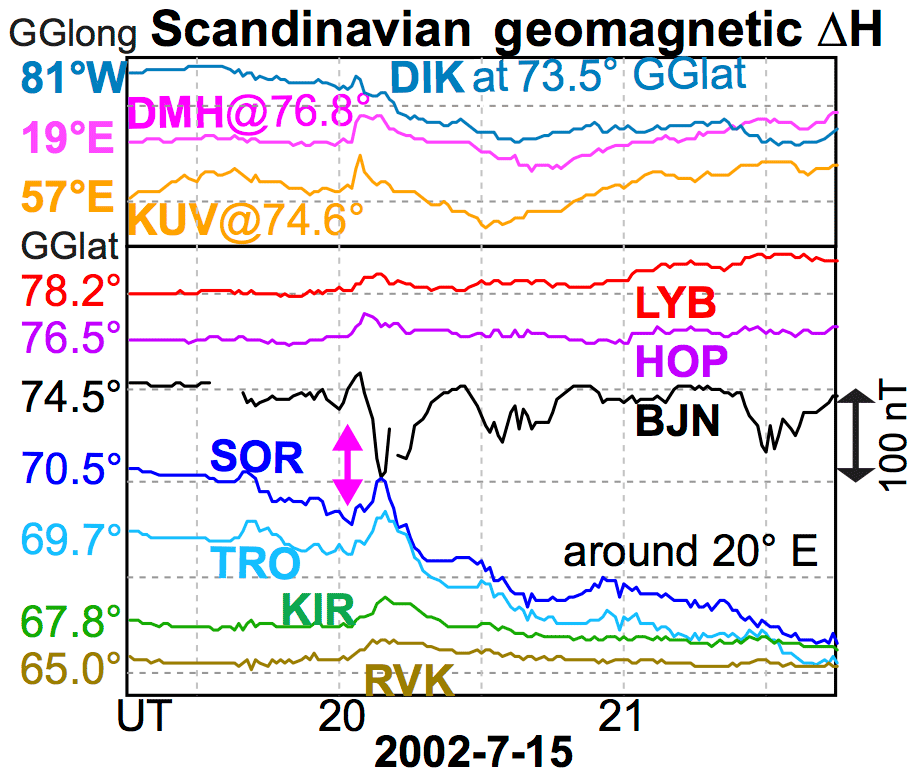
Figure 7 Geomagnetic ΔH in northern Scandinavia and three other stations at around 75^∘ GGlat (stations shown in Fig. 1; Kullorsuaq – KUV) for the X3.0 flare on 15 July 2002. DIK, DMH, and KUV values are approximated by the change in the local magnetic north direction. Red arrows denote the start of the X flare and subsolar crochet. At 20:00 UT, all stations are under sunlight at the ionosphere.

To examine it further, Fig. 7 shows the geomagnetic data on 15 July 2002 at the same stations as Fig. 1. We also added Kullorsuaq (KUV) data from the west coast of Greenland that is located at around 18 MLT at the time of the crochet. In Fig. 7, sudden increases in ΔH at around 20:04 UT are recognised at all stations. In addition, a negative spike started at 20:07 UT at BJN, 20:13 UT at SOR, and at 20:15 UT at TRO. Except for the duration, the ΔH>0 enhancements at high latitudes are similar to what we observed in the 6 September 2017 event (Fig. 1). The short duration is not surprising considering the short duration of high X-ray flux (> M3 class), as indicated in Fig. 6, and the high solar zenith angle (it was about 63^∘ in the Greenland) for this UT.

Since KUV's local time is only 17 LT, which is within the zonal extent of crochet according to DIK's data of the 6 September 2017 event (Fig. 1), this ΔH>0 is quite likely to be the new high-latitude crochet. Then the new high-latitude crochet extends quite widely towards the evening, which is consistent with the season near the summer solstice. Even DIK data (which is located at 01 LT past midnight but still under sunlight) showed a minor signature. This suggests that the AU signature could be caused by this crochet rather than the auroral crochet.

On the other hand, a unique bipolar signature, where the ΔH>0 period is very short, is seen at BJN. This is a candidate for the auroral crochet. In addition, ΔB>0 at SOR, TRO, and DIK can be read as being the disruption of the substorm-related large magnetic bay. In fact, a signature of the small auroral electrojet is seen at BJN, SOR, TRO, and DIK before the crochet (starting at around 19:40 UT). Although the value at BJN returned to normal, and the signature is not visible at Kiruna, a weak aurora existed in this narrow region before the crochet.

However, the auroral electric field before the crochet must be very weak compared to what was reported as the auroral crochet (Pudovkin and Sergeev, 1977), and at least the ΔH>0 signature that is consistently observed at many stations with a precondition of quiet ΔB is better interpreted as the new crochet. Then, we can even wonder if the interaction between the new crochet and the auroral oval accelerated the large ΔB<0 bay.

4 Discussion and future tasks

4.1 Why was this not found in the past?

Although magnetic stations have been extended towards higher latitudes beyond 68^∘ GGlat since 1980s, this new crochet has never been reported, at least not to our knowledge. One possible reason is that the phenomenon is limited to a relatively small range in the geographic latitude (68–75^∘ GGlat), while the station should be completely outside the geomagnetic cusp (<75^∘ Mlat). This criterion excludes many geomagnetic stations over Greenland and Canada from finding the new crochet.

4.2 Need solid statistics and global perspective

There are many questions to answer on this phenomenon. One obvious question regards the conditions that cause this new high-latitude crochet. When we made a survey using quick plots, we compared the indices with the X-ray flux (red lines in Fig. 6) only, but other obvious factors, such as the season and geomagnetic latitude, have not been not sorted out. We thus need to make more solid analyses. For example, we need to include amplitudes (we examined only yes or no responses), examine the closure of the ionospheric current system at high latitudes, analyse global magnetometer network data, and take statistics of them. Such a global perspective would also indicate for which conditions the effect can be detected in AU or AL.

One important note is that the difference between the GGlat and Mlat (i.e. UT dependence) must be considered. Also, we have to note that the current system might be different between different events (the size of the flare may affect the intensity and size, while the season may affect the distribution pattern and profiles of the solar zenith angles of magnetic stations). In addition, if the intensification of the Sq current is important, the new crochet might be enhanced near the equinoxes (rather than summer solstice) through inter-hemispheric coupling (Yamasaki and Maute, 2017), which avoids the saturation of convection-driven charges. Therefore, it might be difficult to obtain consistent results, but at least a common feature can be obtained.

4.3 What is the main driver of the new crochet?

As shown in Fig. 4, this current system might be related to the enhancement of the Sq0-like background current through the enhancement of both the ion and/or electron density and ion velocity (Pedersen electric field). While the density enhancement is explained by the flare radiation, the direct cause of velocity enhancement is not clear. In addition to this obvious question, we need to know the relative importance of these enhancements on the high-latitude crochet, and we need to understand the relation to the nightside crochet because we also found many cases in the nightside as well. This requires identifying the criterion for how to classify the observed crochet as the auroral crochet or nightside extension of the new crochet, which we have not yet found.

To answer these questions, we need similar radar data for different events. Since the availability of radar data in favourable observation modes and geometry (such as the EISCAT data on the 6 September 2017) is limited, we need other radar data, including future facilities such as EISCAT 3D, for a solid answer. Such work will also probably give some hints as to why the electron density decreased at >300 km in Fig. 4. Future satellite missions that cover ionospheric E-region, such as Daedalus (Sarris et al., 2020), are highly necessary.

4.4 Can crochet trigger a substorm or magnetosphere–ionosphere (M–I) coupling?

In the preliminary survey, we found many coincidental cases in which a large gradient of ΔH occurred at the same time as a substorm onset or a sudden intensification of a substorm when the X flare took place. Figure 8 shows one such example, when the X6.2 flare took place at 19:13 UT, and the substorm onset took place immediately after. This substorm is most likely associated with the southward IMF period during 18:29–18:57 UT (not shown here) that is detected at the Sun–Earth first Lagrange point L1 by the Advanced Composition Explorer (ACE), but the triggering mechanism is not necessarily associated with IMF (e.g. Yamauchi et al., 2006). Solar wind density and velocity were stable after the coronal mass ejection (CME) arrival 5 h before, making us consider the crochet as a possible trigger. Larger AU than AL right after the onset is also in agreement with crochet rather than substorm activity because the substorm onset is characterised by large negative ΔH and |AL|≫AU.

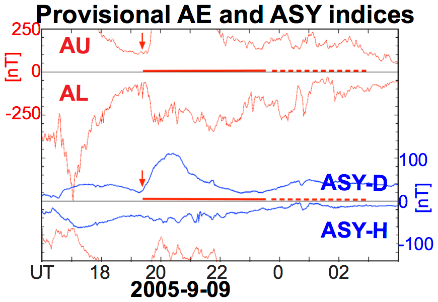
Figure 8 Same format as Fig. 6 for 9 September 2005. A coronal mass ejection (CME) arrived at the Earth at around 13:30 UT, and the IMF turned southward at the Earth at around 19:30 UT.

Theoretically, the crochet mechanism may trigger a substorm through a sudden intensification of ionospheric density and electric field through a magnetosphere–ionosphere (M–I) coupling (e.g. Kan et al., 1988). Since several different onset mechanisms may cause a substorm, it is quite possible that crochet may also trigger a substorm as one of the minor onset mechanisms (Yamauchi, 2019). The investigation of such a scenario is a future task.

The same question arises with respect to the M–I coupling. The latitude range of the new crochet is inside the geomagnetically closed region (near local noon), while it is close to the dayside Region 1 field-aligned current. This means that the new crochet might influence the field-aligned current system. Such a study requires satellite observations at the right location and the right timing.

4.5 Modulation of Pc5?

If the long-lasting high X-ray flux influences the ionospheric current, some effects might arise from the X2.2 flare at 09:00 UT on 6 September 2017, i.e. on the same day as the X9.3 flare (see Fig. 1a). One candidate is the density moderation that synchronises with the Pc5 pulsation during the recovery phase of the substorm that started at 09:37 UT, which peaked at 05:58 UT with $\text{AL}=-\mathrm{666}$ nT (Fig. 2). In fact, ΔH showed large amplitude oscillations with a periodicity of about 30 min during 09:30–11:20 UT (Fig. 1b). However, the electron density at 150–200 km altitudes showed irregular oscillations with a different periodicity (∼15 min), although no modulation is seen at 100 km in altitude. The periodicity in the ion convection is also about 15 min at 150–200 km altitudes. The only candidate that may match with the 30 min periodicity is irregularity in the ion velocity at 100 km altitude, but the profile does not really match with the ΔH variation. This suggests that the Pc5 pulsation can be modulated by the density variation at 150–200 km altitudes.

4.6 Relation to space weather

The large extra ΔH at 68–75^∘ GGlat might, if it happens a during substorm, even be relevant to the space weather hazards because a large sunspot may cause a coincident occurrence of strong solar flare and large substorm powered by the CME. If the crochet mechanism can interact with a substorm, such as reinforcing each other, and if the strong solar flare takes place within 1 h after CME hits the Earth, then we expect extremely strong ionospheric currents and resultant ground-induced currents (GIC) that are hazardous. Thus, crochet study is potentially related to other research fields.

5 Conclusions

Using magnetometer data from northern Europe, Russia, and Greenland, as well as EISCAT data, we found a new type of solar flare effect (SFE, or crochet) on the geomagnetic disturbance in response to the X9.3 flare on 6 September 2017 at high latitudes (65–75^∘ GGlat). The new crochet is located at higher latitudes than the subsolar crochet (see Figs. 4b and 4d), and it is found over a wide local time range, including local noon but outside the cusp, i.e. in the geomagnetic closed region. It lasted for a longer duration, with higher peak amplitudes than the subsolar crochet. The equivalent ionospheric current flows eastward in a limited latitude range but extended over at least 8 h in local time (LT), forming a zonal current region at around 70–75^∘ GGlat (equatorward of the polar cap – at least in dayside). Considering its location and duration, this crochet is different from previously studied crochets (subsolar, auroral, and cusp).

Ionospheric parameters at local noon during this crochet show strong background ion convection before the crochet, and also show a sharp enhancement of the electron density (and, hence, the ion-neutral density ratio) during the crochet. Thus, the new crochet can be related to an increase in electron density at 100–150 km altitudes, where the strong background (Sq0) ion convection exists. For example, a change in the E-layer height can actually cause the ionospheric current at high latitudes, but such a scenario does not easily explain why it is found in a limited latitudinal range, and therefore, the mechanism is still unclear.

We also examined the crochet signatures in AE and ASY indices for all X flares (> X2.0) over the past two solar cycles. While the subsolar crochet is well recognised in ASY indices, the crochet signatures that represent the new crochet or auroral crochet are also recognised in AU for half of the cases and even in AL sometimes. However, the AE index alone cannot distinguish between this new crochet and the auroral crochet in the evening sector, and further studies are needed to understand the current system related to these crochets.