the Creative Commons Attribution 4.0 License.
the Creative Commons Attribution 4.0 License.
 | 29 Oct 2020
An inter-hemispheric seasonal comparison of polar amplification using radiative forcing of a quadrupling CO2 experiment
Fernanda Casagrande
Ronald Buss de Souza
Paulo Nobre
Andre Lanfer Marquez
The numerical climate simulations from the Brazilian Earth System Model (BESM) are used here to investigate the response of the polar regions to a forced increase in CO2 (Abrupt-4×CO2) and compared with Coupled Model Intercomparison Project phase 5 (CMIP5) and 6 (CMIP6) simulations. The main objective here is to investigate the seasonality of the surface and vertical warming as well as the coupled processes underlying the polar amplification, such as changes in sea ice cover. Polar regions are described as the most climatically sensitive areas of the globe, with an enhanced warming occurring during the cold seasons. The asymmetry between the two poles is related to the thermal inertia and the coupled ocean–atmosphere processes involved. While at the northern high latitudes the amplified warming signal is associated with a positive snow– and sea ice–albedo feedback, for southern high latitudes the warming is related to a combination of ozone depletion and changes in the wind pattern. The numerical experiments conducted here demonstrated very clear evidence of seasonality in the polar amplification response as well as linkage with sea ice changes. In winter, for the northern high latitudes (southern high latitudes), the range of simulated polar warming varied from 10 to 39 K (−0.5 to 13 K). In summer, for northern high latitudes (southern high latitudes), the simulated warming varies from 0 to 23 K (0.5 to 14 K). The vertical profiles of air temperature indicated stronger warming at the surface, particularly for the Arctic region, suggesting that the albedo–sea ice feedback overlaps with the warming caused by meridional transport of heat in the atmosphere. The latitude of the maximum warming was inversely correlated with changes in the sea ice within the model's control run. Three climate models were identified as having high polar amplification for the Arctic cold season (DJF): IPSL-CM6A-LR (CMIP6), HadGEM2-ES (CMIP5) and CanESM5 (CMIP6). For the Antarctic, in the cold season (JJA), the climate models identified as having high polar amplification were IPSL-CM6A-LR (CMIP6), CanESM5(CMIP6) and FGOALS-s2 (CMIP5). The large decrease in sea ice concentration is more evident in models with great polar amplification and for the same range of latitude (75–90∘ N). Also, we found, for models with enhanced warming, expressive changes in the sea ice annual amplitude with outstanding ice-free conditions from May to December (EC-Earth3-Veg) and June to December (HadGEM2-ES). We suggest that the large bias found among models can be related to the differences in each model to represent the feedback process and also as a consequence of each distinct sea ice initial condition. The polar amplification phenomenon has been observed previously and is expected to become stronger in the coming decades. The consequences for the atmospheric and ocean circulation are still subject to intense debate in the scientific community.
- Article
(4783 KB) - Full-text XML
- BibTeX
- EndNote


Polar regions have been shown to be more sensitive to climate change than the rest of the world (Smith et al., 2019; Serreze and Barry, 2011). The Arctic is warming at least twice as fast as the Northern Hemisphere and as the globe as a whole. This phenomenon is known as the Arctic amplification (AA) and is combined with a fast shrinking of the sea ice cover (Serreze and Barry, 2011; Kumar et al., 2010; Screen and Simmonds, 2010). Previous research has indicated that the enhanced Arctic warming is a response to anthropogenic greenhouse gas (GHG) forcing, which, in turn, intensifies many complex nonlinear coupled ocean–atmosphere feedbacks (e.g., the sea ice–albedo feedback) (Stuecker et al., 2018; Pithan and Mauritsen, 2014; Alexeev et al., 2005). The sea ice–albedo feedback is one of the key mechanisms in amplifying Arctic warming, playing an important role in global climate change (Stuecker et al., 2018; Pithan and Mauritsen, 2014). In contrast to the Arctic sea ice, the total sea ice cover surrounding the Antarctic continent has increased in association with cooling over eastern Antarctica and warming over the Antarctic Peninsula. The physical ocean–atmosphere coupled processes responsible for Antarctic sea ice rising are still unclear. Turner et al. (2017) show the unprecedented springtime retreat of Antarctic sea ice in 2016. However, results derived from numerical simulations and observations point to a combination of changes in the wind pattern, the ocean circulation, accelerated basal melting of Antarctica's ice shelf and the ozone depletion (Marshall et al., 2014; Bintanja et al., 2013; Thompson et al., 2011; Thompson and Solomon, 2002). According to Marshall et al. (2014), these two-pole inter-hemispheric asymmetries strongly influence the sea surface temperature (SST) response to an increase in the global CO2 forcing, accelerating the warming in the Arctic while delaying it in Antarctica.
Numerous scientific publications based on both observations and state-of-the-art global climate model simulations for the high latitudes of the Northern Hemisphere have shown that AA is an intrinsic feature of the Earth's climate system (Smith et al., 2019; Vaughan et al., 2013; Serreze and Barry, 2011; Screen and Simmonds, 2010). These works suggested that the surface air temperature (SAT) will continue to increase, with effects extending beyond the Arctic region (Dethloff et al., 2019; Smith et al., 2019; Bintanja et al., 2013; Serreze and Barry, 2011; Winton, 2006; Holland and Bitz, 2003). Although the annual average SAT at northern mid and high latitudes is increasing, the wintertime SAT has decreased since 1990 (Zhang et al., 2016; Mori et al., 2014; Cohen et al., 2012; Honda et al., 2009).
Bekryaev et al. (2010), for instance, found a warming rate of 1.36 ∘C century−1 for the period from 1875 to 2008 using an extensive set of observational data from meteorological stations located at high latitudes of the Northern Hemisphere (>60∘ N). That trend is almost double that of the Northern Hemisphere trend as a whole (0.79 ∘C century−1), with an accelerated warming rate in the most recent decade. Rigor et al. (2002), also using an observational dataset, showed that the Arctic warming varies largely among regions and that changes in SAT are also related to the Arctic Oscillation (Ambaum et al., 2001).
The Arctic Ocean temperature and ocean heat fluxes also have increased over the past several decades (Walsh, 2014; Polyakov et al., 2010, 2008). According to Polyakov et al. (2017), the recent sea ice shrinking, weakening of the halocline and shoaling of the intermediate–deep Atlantic water mass layer in the eastern Eurasia basin have increased the winter ventilation in the ocean interior, making the region structurally similar to the western Eurasian basin. The authors described these processes as an “Atlantification” phenomenon and represent an essential step toward a new Arctic climate state.
Holland and Bitz (2003), using a set of 15 state-of-the-art CMIP models, found that the range of simulated Arctic warming as a response to a doubling of CO2 concentration varies largely between the models ranging from 1.5 to 4.5 times the global mean warming. The large differences among the models are related to differences in simulating the ocean's meridional heat transport, the polar cloud cover and the sea ice (e.g., a simulation with thinner sea ice cover presents a higher polar amplification).
According to Shu et al. (2015), global climate models in general offer much better simulations for the Arctic than for the Antarctic. Turner et al. (2015) suggested that the main problem of climate models at the high latitudes of the Southern Hemisphere is their inability to reproduce the observed (although slight) increase in sea ice extent (SIE). Bintanja et al. (2015) and Swart and Fyfe (2013) have demonstrated the importance of including the effect of the increasing freshwater input from Antarctic continental ice into the Southern Ocean. The authors showed that the ice sheet dynamics, essential for having accurate sea ice simulations, is currently disregarded in all CMIP5 models. Swart and Fyfe (2013) also suggested that this deficiency may significantly influence the simulated sea ice trend because the subsurface ocean warming causes basal ice-shelf melt, freshening the surface waters, which eventually leads to an increase in sea ice formation. Moreover, the instrumental network for data collection in Antarctica and the Southern Ocean is considered scarce (even more than in the Arctic), inhomogeneous and insufficiently dense to validate climate models. Therefore, for the high-latitude regions of the Southern Hemisphere, the effects of the ongoing climate change and its associated processes are still considered hot topics that lack conclusive answers.
How the polar climate will change as a response to an external forcing deeply depends on feedback processes, which operate to amplify or diminish the effects of climate change forcing. These feedbacks depend on the integrated coupled processes between the ocean–atmosphere–cryosphere over a large spectrum of spatial and temporal scales, which makes the quantification of them even more complicated.
Here the seasonal sensitivity of high latitudes as a response to quadrupling atmospheric CO2 is investigated using the recently developed Brazilian Earth System Model, coupled ocean–atmosphere version 2.5 (BESM-OA V2.5), and comparing its results with those from 32 other coupled general circulation models participating in CMIP5 and CMIP6. Our goal is to investigate the coupled processes underlying the polar warming by seasons. The paper is organized as follows: Sect. 2 provides a description of the climate models and experimental design(s) used in this work, focusing on the BESM-OA V2.5 model (Veiga et al., 2019; Giarolla et al., 2015; Nobre et al., 2013). In Sect. 3, the seasonality in the surface warming at high latitudes is examined of both the Northern Hemisphere and Southern Hemisphere, and results from the different models are compared. Section 4 provides an analysis of the vertical structure of air temperature warming, the spatial pattern of sea ice changes and a discussion about the coupled ocean–atmosphere processes and feedback mechanisms involved. A summary of the results and conclusions are presented in Sect. 5.
2.1 Numerical design
This study used two numerical experiments from CMIP5 and CMIP6: (i) piControl: it runs for 700 years, forced by an invariant pre-industrial atmospheric CO2 concentration level (280 ppmv); and (ii) Abrupt-4×CO2: it runs for 460 years, comprising an abrupt instantaneous quadrupling of atmospheric CO2 level concentration from the piControl simulation. The design of both experiments follows the CMIP5 protocol (Taylor et al., 2012) and Eyring et al. (2016) for the CMIP6 numerical experiments.
Although an instantaneous quadrupling CO2 scenario is not realistic for the 21st century compared with RCP scenarios and observations, this scenario can give us a measure of climate sensitivity and how large the response of the polar region in comparison to the globe can be as a whole. The results are compared for polar amplification (changes in air temperature) and sea ice cover for the same numerical experiment.
For CMIP5 numerical experiments, the following models are used: BESM-OA V2.5 (Nobre et al., 2013; Veiga et al., 2019), ACCESS-3 (Bi et al., 2013; Collier and Uhe, 2012), GFDL-ESM2M (Griffies, 2012), IPSL-CM5-LR (Dufresne et al., 2013), MIROC-ESM (Watanabe et al., 2011), MPI-ESM-LR (Stevens et al., 2013), NCAR-CCSM4 (Gent et al., 2011), CanESM2 (Chylek et al., 2011), FGOALS-s2 (Bao et al., 2013), GFDL-ESM2G (Delworth et al., 2006), GISS-E2_H (Schmidt et al., 2006), HadGEM2-ES (Collins et al., 2008), MIROC5 (Watanabe et al., 2010), MPI-ESM-P (Giorgetta et al., 2013), and MRI-CGCM3 (Yukimoto et al., 2012).
For CMIP6 numerical experiments, the following models are used: ACCESS-CM2 (Bi et al., 2013), CAMS-CSM1-0 (Rong, 2019), CanESM5 (Swart et al., 2019), CMCC-CM2-SR5 (Fogli et al., 2019), CNRM-ESM2-1 (Séferian et al., 2019), ACCESS-ESM1-5 (Ziehn et al., 2019), E3SM-1-0 (Bader et al., 2019), EC-Earth3-Veg and FGOALS-G3 (Li et al., 2020), GISS-E2-1-H (Schmidt et al., 2006), INM-CM4-8 (Volodin et al., 2019), MIROC6 (Tatebe et al., 2018), MIROC-ES2L (Hajima et al., 2020), MPI-ESM1-2-LR (Fiedler et al., 2019), and MRI-ESM2-0 (Yukimoto et al., 2019).
2.2 Brazilian Earth System Model
The Brazilian Earth System Model, Version 2.5 (BESM-OA2.5) used here is a global climate coupled ocean–atmosphere–sea ice model and is part of the CMIP5 project. The atmospheric component of BESM-OA2.5 is BAM (Brazilian Atmospheric Model) and was described in detail by Figueroa et al. (2016). The latest version of BAM, used here and described by Figueroa et al. (2016) and Veiga et al. (2019), has spectral horizontal representation truncated at triangular wave number 62, a grid resolution of approximately , and 28σ levels in the vertical, with unequal increments between the vertical levels (i.e., a T62L28). Two important changes were implemented in the BESM latest version: (i) a new microphysics scheme, described by Ferrier et al. (2002) and Capistrano et al. (2020), and (ii) a new surface layer scheme, described by Capistrano et al. (2020) and Jimenez and Dudhia (2012). These key changes represent an improvement in the surface layer, resulting in better representation of near-surface air temperature, wind and humidity at 10 m. The main improvements occur over the ocean, where temperature, wind and humidity are important for calculating the heat fluxes at the ocean–atmosphere–sea ice interface.
The oceanic component of BESM-OA2.5 is the Modular Ocean Model, Version 4p1, from the National Oceanic and Atmospheric Administration-Geophysical Fluid Dynamics Laboratory (MOM4p1/NOAA-GFDL), described in detail by Griffies (2009). The MOM4p1 includes a Sea Ice Simulator (SIS) built-in ice model (Winton, 2000). The SIS has five ice thickness categories and three vertical layers (one snow and two ice). To calculate ice-internal stresses, the elastic–viscous–plastic technique described by Hunke and Dukowicz (1997) was used. The thermodynamics is given by a modified Semtner three-layer scheme (Semtner, 1976). SIS is able to calculate sea ice concentrations, snow cover, thickness, brine content and temperature. The horizontal grid resolution of MOM4p1 in the longitudinal direction is set to 1∘. The latitudinal direction varies uniformly, in both hemispheres, from 1∕4∘ between 10∘ S and 10∘ N to 1∘ in resolution at 45∘ and to 2∘ in resolution at 90∘. The vertical axis has 50 levels (the upper 220 m have 10 m resolution, increasing to about 360 m at deeper levels). The MOM4p1 and BAM models were coupled using an FMS coupler. FMS coupled was developed by NOAA-GFDL. The BAM model receives SST and ocean albedo from MOM4p1 and SIS (hour by hour). The MOM4p1 receives momentum fluxes, specific humidity, pressure, heat fluxes, vertical diffusion of velocity components and freshwater. The Monin–Obukhov scheme is used to calculate the wind stress fields.
First we discuss the seasonality of polar warming near the surface in the Arctic, vertical profile, sea ice changes, differences among models and coupled process involved. Afterwards, we do the same analysis for the southern high latitudes and assess the reasons for asymmetries between poles.
3.1 Polar amplification
In order to evaluate the seasonality of near-surface polar warming, the seasons are defined as follows: December to February (DJF) as boreal winter, March to May (MAM) as boreal spring, June to August (JJA) as boreal summer, and September to November (SON) as boreal fall.
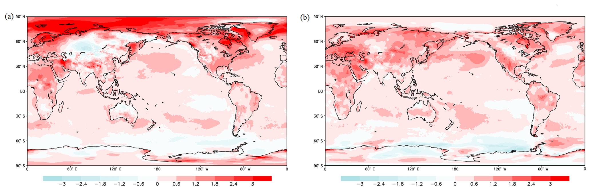
Figure 1Polar amplification using long-term observations of surface air temperatures (∘C) for 2008–2018 (seasonal average) relative to 1979–1989 (seasonal average) in (a) winter (DJF) and (b) summer (JJA). Source: ERA-Interim Reanalysis.
Figure 1 shows the enhanced surface warming at high latitudes compared to the rest of the globe, with a slightly greater rate of warming in the 20th century. This polar amplification is not symmetric; most evidence is from the Arctic region (during the boreal winter). According to Stocker et al. (2013), the enhanced warming at northern high latitudes was linked to a decrease in snow cover and sea ice concentration, sea level rise and an increase in land precipitation. Furthermore, there were changes in atmospheric and ocean circulations (Pedersen et al., 2019; Pithan and Mauritsen, 2014; Stocker et al., 2013; Yang et al., 2010; Graversen et al., 2008). Polar amplification is also reported by climate models, driven by solar or natural carbon cycle perturbations (Sundqvist et al., 2010; O'ishi et al., 2009; Mann et al., 2009; Masson-Delmotte et al., 2006).
Figures 2 and 3 show the seasonality of the polar amplification (change in zonal SAT average) simulated by BESM-AO V2.5 and 32 state-of-the-art CMIP5 and CMIP6 models. To assess the climate sensitivity of polar amplification and seasonal and coupled processes involved, we used the difference between Abrupt-4×CO2 and piControl numerical experiments, considering only the last 30 years of the 150 years of model integration after quadrupling CO2 concentration (when the model reaches a new equilibrium state). This procedure has been largely used by researchers, since it allows us to evaluate and compare potential warming and sensitivities among low and high latitudes as well as to compare differences between models (Van der Linden et al., 2019; Cvijanovic et al., 2015; Manabe et al., 2004; Holand and Bitz, 2003).
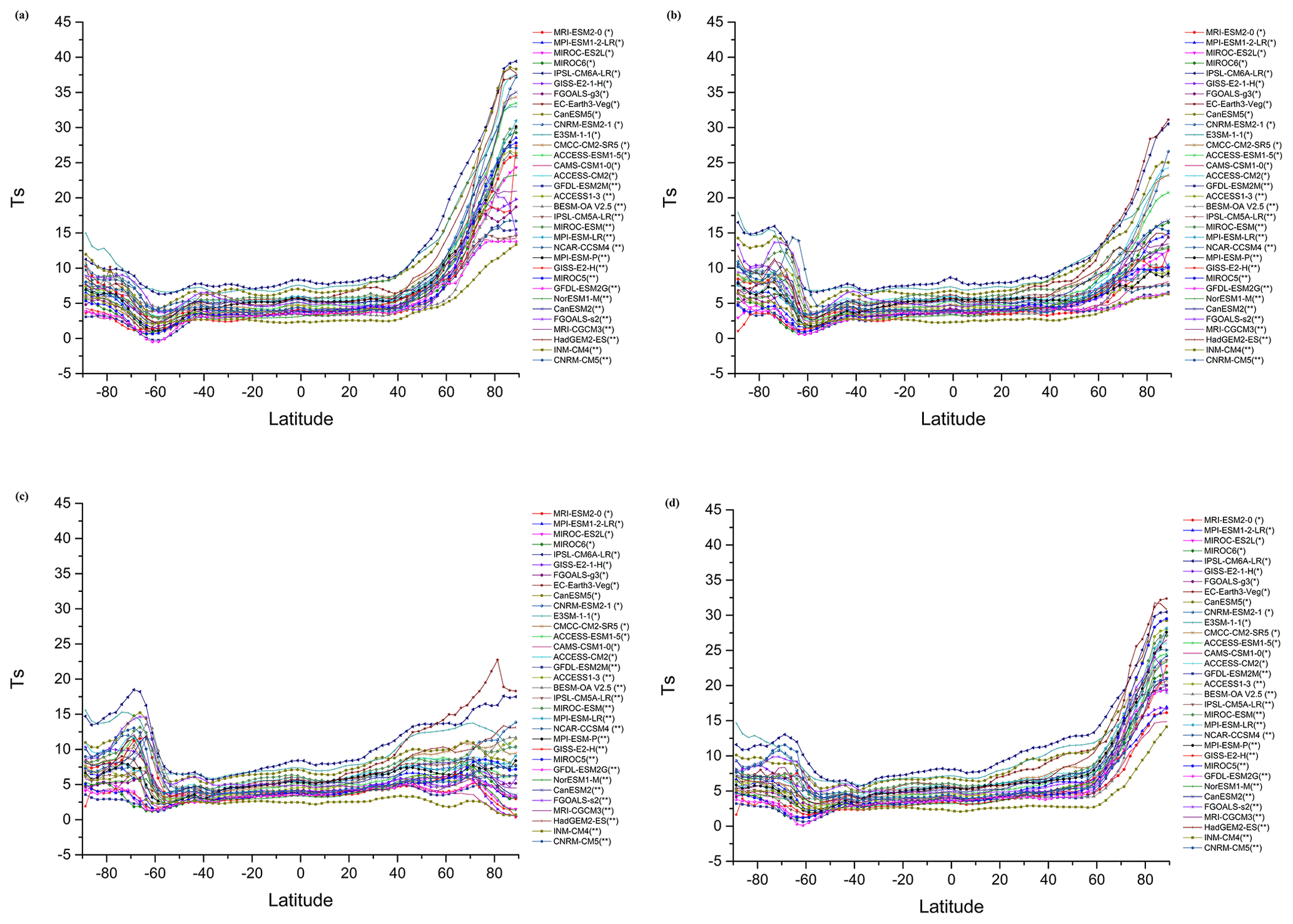
Figure 2Seasonal zonal mean surface temperature differences (K) for the last 30 years of the Abrupt-4×CO2 numerical experiment minus the last 30 years of the piControl run for the CMIP5 and CMIP6 models for (a) winter (DJF), (b) spring (MAM), (c) summer (JJA) and (d) fall (SON).
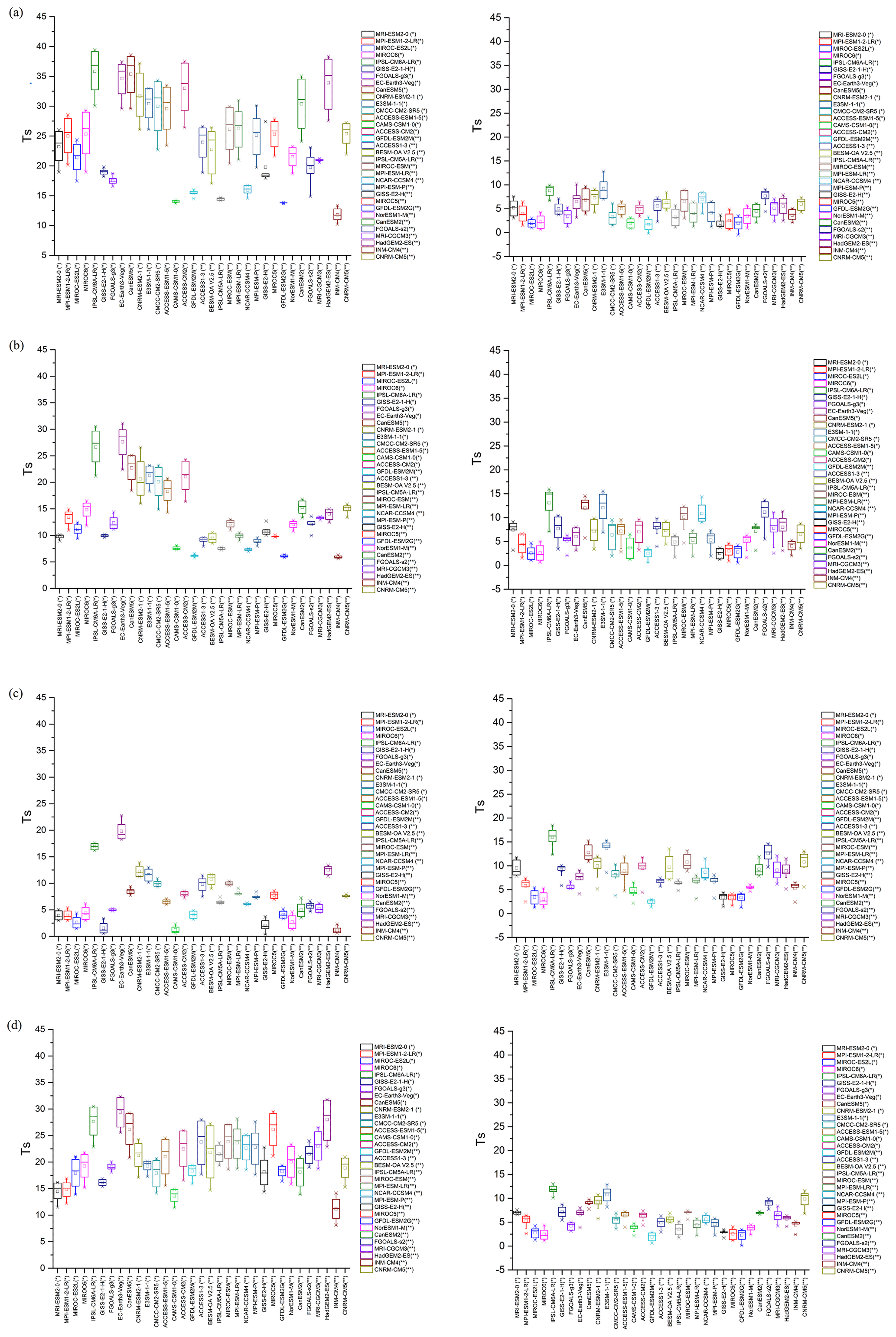
Figure 3Seasonal zonal mean surface temperature differences (K) for the last 30 years of the Abrupt-4×CO2 numerical experiment minus the last 30 years of the piControl run for the CMIP5 and CMIP6 models; box plot in 75–90∘ N (left) and 60–80∘ S (right) for (a) winter (DJF), (b) spring (MAM), (c) summer (JJA) and (d) fall (SON).
Under the largest future GHG forcing (4×CO2), the polar regions are found to be the most sensitive areas of the globe, with a very pronounced seasonality (Figs. 2 and 3). The high southern latitude warming predicted by the models analyzed is modest in relation to the Arctic's but is still not negligible. This asymmetry is partly due to the smaller area covered by the ocean in the Northern Hemisphere that induces a smaller thermal inertia. In contrast to the high latitudes, the tropical warming is similar for both hemispheres, without the robust warming pattern as shown at high latitudes. Salzmann (2017) suggested that the overall weaker warming in Antarctica is due to a more efficient ocean heat uptake in the Southern Ocean, weaker surface–albedo feedback in combination with ozone depletion. The BESM-OA V2.5 model has no ozone chemistry as a climate component, so we suggest that, even neglecting the ozone depletion, the weaker warming in Antarctica will be shown. A weak albedo–sea ice feedback is also expected compared with the Arctic region (because of the fast retreat of sea ice in the Northern Hemisphere). The role of the Antarctica surface height in both feedback processes and meridional transports is similarly important to consider. According to Salzmann (2017), the polar amplification asymmetry is explained by the difference in surface height. If Antarctica is considered to be flat in a climate simulation with the CO2-doubling experiment, the north–south asymmetry is reduced.
From September to February (boreal fall and winter), the surface warming is maximum at northern high latitudes, decreasing with latitude to reaching a minimum at 60∘ S and then increasing towards the South Pole. Consistent with previous analyses based on climate simulations and observations, this enhanced Arctic amplification appears as an inherent characteristic for the Arctic region (Pithan and Mauritsen, 2014). From March to August, the reverse signal shows the maximum warming close to 70∘ S, decreasing towards to the tropical region and lacking the enhanced warming at the northern high latitudes.
The main reason for winter (DJF) Arctic amplification pointed out by Serreze et al. (2009) is largely driven by changes in sea ice, allowing for intense heat transfers from the ocean to the atmosphere. During boreal summer, when Arctic warming is not prominent and solar radiation is maximal, the energy is used to melt sea ice and increase the sensible heat content of the upper ocean. The atmosphere heats the ocean during summer, whereas the flux of heat is reverse in winter. The sea ice loss in summer allows a large warming of the upper ocean, but the atmospheric warming at the surface or lower troposphere is modest (promoting more open water). The excess heat stored in the upper ocean is subsequently released to the atmosphere during winter (Serreze et al., 2009). According to Lu and Cai (2009), in summertime the positive surface–albedo feedback is mainly canceled out by the negative cloud radiative forcing feedback. The positive surface–albedo feedback is relatively much weaker in winter when compared to its counterpart in summer; therefore, it does not contribute to the pronounced polar amplification in winter.
For southern high latitudes, a pronounced warming appears from March to August (boreal summer and spring), predominantly close to 70∘ S. This enhanced warming tends to decrease in the direction of the South Pole. This pattern is similar to the one obtained by Goosse and Renssen (2001). The authors used a coupled climate model to investigate the response of the Southern Ocean to an increase in GHG concentration. They found that the response could occur separately in two distinct phases. At the first moment, the ocean damps the surface warming (because of its large heat capacity). Then, after 100 years of run simulation, the warming is enhanced due to a positive feedback that is linked to a stronger oceanic meridional heat transport toward the Southern Ocean.
When comparing the seasonal response to CO2 forcing among the CMIP5 and CMIP6 models, for boreal winter (DJF), the enhanced Arctic warming at 75–90∘ N is shown to be a robust feature of all CMIP5 and CMIP6 climate model simulations presented here. For the high Northern Hemisphere (high Southern Hemisphere), the warming (difference between piControl and 4×CO2) ranged from 10 to 39 K (−0.5–13 K). CAMS-CSM1-0 (CMIP6) and INMC-CM4 (CMIP5) presented the lowest warming, close to 12 K for northern high latitudes. On the other hand, IPSL-CM6A-LR (CMIP6), HadGEM2-ES (CMIP5) and CanESM5 (CMIP6) outputs presented warming almost twice as large, with a high amplification close to 30 K. The BESM model, for the winter (DJF) season, presented polar amplification for northern high latitudes, close to 27 K.
One interesting feature shown in Fig. 2 is related to the maximum Arctic warming obtained in different simulations. Many models have shown that the maximum warming does not always occur at the highest northern latitudes; instead, it occurs between 80 and 85∘ N, decreasing toward 90∘ N. According to Holland and Bitz (2003), the localization of the maximum warming varies widely among CMIP outputs, but models with high polar amplification generally presented a maximum warming over the Arctic basin. Therefore, we suggest that the spatial distribution of maximum Arctic amplification can be closely related to sea ice conditions though a sea ice–albedo feedback, and this region (Arctic basin) presents the major taxes of decrease in sea ice concentration. A similar result was found for the sea ice simulation from the BESM model, as discussed below (Fig. 5 and Table 1). Additionally, Casagrande et al. (2016), using the BESM-OA V2.3 model, showed that the sea ice spatial pattern could vary largely between the CMIP5 models, especially in frontier areas.
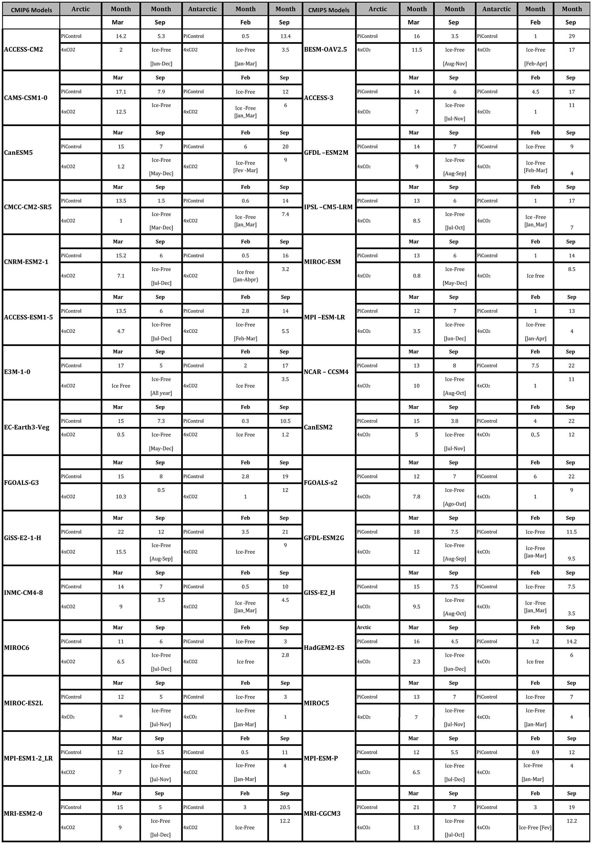
Table 1Climatology of maximum and minimum sea ice area (million square kilometers) for the last 30 years of the Abrupt-4×CO2 numerical experiment and the last 30 years of the piControl run for the CMIP5 and CMIP6 models.
For the southern high latitudes, in wintertime (DJF – Fig. 2), the warming decreases to close to 60∘ S for most CMIP5 and CMIP6 models, increasing toward the South Pole, with the maximum warming close to 11 K. The minimum warming is registered by GFDL-ESM2M and GFDL-ESM2G, both from CMIP5 simulations (close to 0 K in 60∘ S) and the maximum South Pole amplification between models is presented by E3SM-1, close to 90∘ S. In summer (JJA), the compared response to CO2 forcing in CMIP5 models is amplified (damped) in the Southern (Northern) Hemisphere. A pronounced amplification was found close to 70∘ S with a range of 1 to 17 K, decreasing towards the South Pole. In this region the maximum was obtained by the BESM-OA V2.5 model, close to 13 K.
The pronounced seasonality of near-surface warming in polar regions has been found in observations (Bekryaev et al., 2010) and climate simulations (Holland and Bitz, 2003), but less emphasis has been placed on the vertical structure of the atmosphere. To understand whether this enhanced warming occurs only in the surface or also well above, Fig. 4 presents results obtained with three different CMIP5 models with moderate (BESM-OA V2.5/MPI-ESM-LR) and low (NCAR-CCSM4) polar amplification (based on Figs. 2 and 3).

Figure 4Zonal-average atmosphere temperature changes, in ∘C (Abrupt-4×CO2 minus piControl) at each pressure level and in mb (solid line) for the last 30-year run for (a) BESM OA V2.5, (b) NCAR-CCSM4 and (c) the MPI-ESM-LR model, in DJF (left column) and JJA (right column).
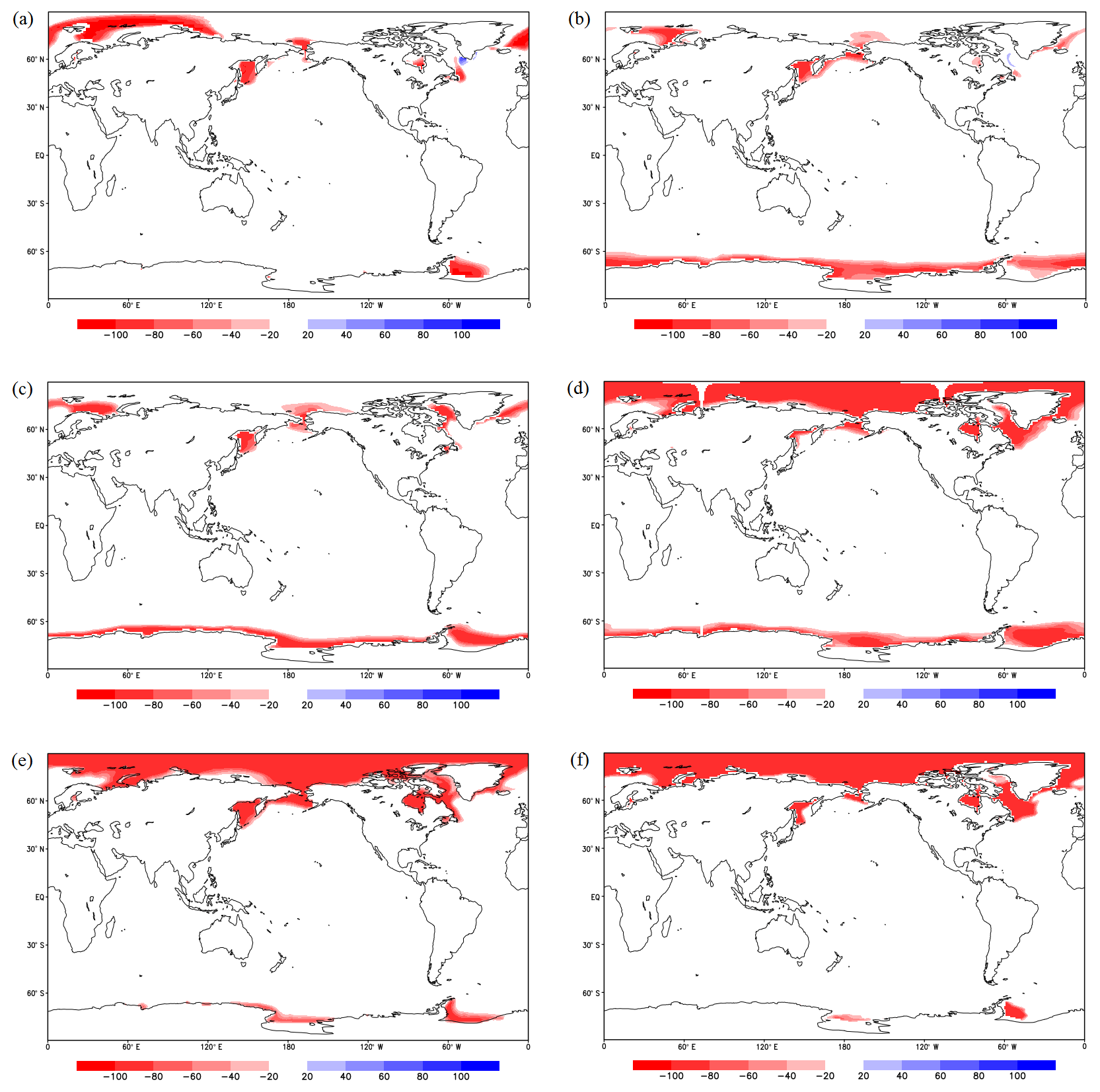
Figure 5Sea ice concentration for the last 30 years of the Abrupt-4×CO2 numerical experiment minus the last 30 years of the piControl run for the following models: (a) BESM-OA V2.5, (b) NCAR-CCSM4, (c) FGOALS-S2, (d) CanESM5, (e) HadGEM2-ES and (f) EC-Earth3-Veg in March (left column).
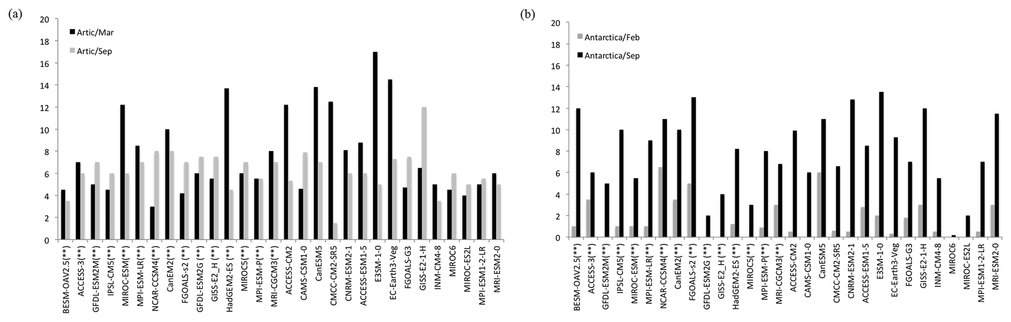
Figure 6Climatology of maximum and minimum sea ice area (million square kilometers) for the last 30 years of the Abrupt-4×CO2 numerical experiment minus the last 30 years of the piControl run for the CMIP5 and CMIP6 models. (a) Arctic: black colors represent March and gray colors represent September; (b) Antarctic: black colors represent September and gray colors represent February.
Figure 4 shows evidence of temperature amplification well above the surface, with enhanced warming during the cold season for both northern and southern high latitudes. Snow and ice feedback cannot explain the warming above the lowermost part of the atmosphere because this feedback is expected to primarily affect the air temperature near the surface. Part of the vertical warming may be explained by physical mechanisms that induce warming as changes in the atmospheric heat transport into the Arctic. According to Graversen et al. (2008), a substantial proportion of the vertical warming can be caused by changes in this variable, especially in summertime (JJA). Graversen and Wang (2009) used an idealized numerical experiment (doubling CO2) with a climate model that has no ice–albedo feedback. Their results also revealed a polar warming as a response to anthropogenic forcing (doubling CO2). It was found that the enhanced Arctic warming is due to an increase in the atmospheric northward transport of heat and moisture. These results are supported by observational and numerical analyses (Graversen et al., 2014, 2008). In addition to ice–albedo feedback, the strength of the atmospheric stratification is an important factor in explaining the vertical warming. The troposphere is more stably stratified at high latitudes. An increase in GHG forcing generates an increase in downwelling longwave radiation at the surface, consequently causing warming, which in polar regions is confined to the lower troposphere (Graversen et al., 2014, 2009).
When examining Arctic warming at different levels computed by the three different models shown in Fig. 4, we find that MPI-ESM-LR presented the strongest warming in both near-surface temperature and at high levels. Similar behavior is found at tropical regions, with robust warming at high levels (400–200 hPa). Holland and Bitz (2003) suggested that sea ice conditions are more important than continental ice and snow cover for enhanced polar warming. According to these authors, models with relatively thin sea ice in the control run tend to have higher warming. The same feature was found in BESM-OA V2.5. According to Casagrande et al. (2016) and Casagrande (2016), the last version of the BESM model (Version 2.5) is considered to be a climate model with high polar amplification exhibiting thin sea ice conditions in the control run. This occurs, in part, because of the new surface scheme based on Jimenez and Dudhia (2012) and the microphysics of Ferrier et al. (2002). The advantage of these changes in the BESM's last version is an improvement in the representation of precipitation, wind and humidity in tropical regions. Comparatively, NCAR-CCSM4 is considered a model with moderate polar amplification for both the Northern and Southern oceans. The warming at high levels in boreal summer is not as amplified as in boreal winter. These results are in agreement with Holland and Bitz (2003).
Figure 5 shows, under the largest future GHG (4×CO2), the spatial pattern of sea ice changes for both the Arctic and Antarctic (difference between sea ice concentration for the last 30 years of the Abrupt-4×CO2 numerical experiment and the last 30 years of the piControl run). The maximum of the Arctic warming obtained from observations (Fig. 1) and different CMIP5 simulations (Figs. 2 and 3) occurs in boreal winter (DJF).
According to Fig. 2, the following models, in descending order, appear as having greater amplification: IPSL-CM6A-LR (CMIP6), HadGEM2-ES (CMIP5) and CanESM5 (CMIP6). A similar response, for the same period, is observed in Figs. 5 and 6, related to sea ice changes. Figure 6 shows the climatology of maximum and minimum sea ice area for the last 30 years of the Abrupt-4×CO2 numerical experiment minus the last 30 years of the piControl run. For the Arctic, in March, EC-Earth3-Veg (NCAR-CCSM4) shows the highest (lowest) value, close to km2 (3×10⁶ km2). For September, in agreement with Fig. 2, the polar amplification is not evident as in the cold period. For Antarctica (Fig. 6), in the cold period (September), the difference between the Abrupt-4×CO2 numerical experiment and the piControl run is higher for models with enhanced polar amplification, as FGOALS-S2 ( km−2). Both Figs. 5 and 6 and Table 1 are in agreement with Fig. 2, showing that the large decrease in sea ice concentration is more evident in models with great polar amplification and for the same range of latitude (75–90∘ N). The end of the melting period (when sea ice reaches its minimum annual value) for all models shows sea ice-free conditions (Table 1). Models that have strong polar amplification also exhibit expressive changes in the annual amplitude of sea ice with outstanding ice-free conditions from May to December (EC-Earth3-Veg) and June to December (HadGEM2-ES). Then, the end of the melting period is expected early, likely associated with a large decrease in sea ice thickness, which contributes to a delay in sea ice formation. For BESM-OA V2.5, Arctic ice-free conditions are found from August to November. We suggest that the Arctic will become covered only by first-year sea ice (more vulnerable to melting), making the region more sensitive thermodynamically and dynamically to temperature changes. This evidence corroborates the theory that the Arctic polar amplification is closely linked to sea ice–albedo feedback. For Antarctica, however, the same physical processes cannot be used to explain the polar amplification (as discussed previously). Although, according to Figs. 2 and 4, there is a small indication of the contribution of sea ice–albedo feedback in Antarctic polar amplification, this still remains an open discussion, and we suggest that is important to consider the contribution of the ice sheet in polar amplification.
Previous researchers, using observational and modeling datasets, have found that shrinking of sea ice (Fig. 5) and enhanced Arctic warming may affect the middle latitudes (Coumou et al., 2018; Screen, 2017; Walsh, 2014). According to Walsh (2014), the AA acts by weakening the west-to-east wind speed in the upper atmosphere, by increasing the frequency of wintertime blocking events that in turn lead to persistence or slower propagation of anomalous temperature at middle latitudes, and by increasing the continental snow cover, which can in turn influence the atmospheric circulation. Finally, in view of the results, it is important to consider the limitations and differences among each climate model in order to improve the understanding of the physical process in climate simulations that represent large biases among the models belonging to the CMIP5 project.
Polar amplification is possibly one of the most important sensitive indicators of climate change. Robust patterns of near-surface temperature response to global warming at high latitudes have been identified in recent studies (Smith et al., 2019; Stuecker et al., 2018; Pithan and Mauritsen, 2014). For northern high latitudes, the shrinkage of sea ice as a response to an increase in GHC is one of the most cited reasons (Serreze and Barry, 2011; Kumar et al., 2010; Screen and Simmonds, 2010). Here we analyzed the seasonality of polar amplification using some CMIP5 coupled climate models in a quadrupling CO2 numerical experiment for both the Northern Hemisphere and Southern Hemisphere. Our results showed that the polar regions are much more vulnerable to a large warming due to an increase in atmospheric CO2 forcing than the rest of the world, particularly during the cold season. For northern high latitudes, the albedo–sea ice feedback contributes to a decrease in sea ice cover, exposing new expanses of ocean and land surfaces (leading to greater solar absorption), thus amplifying the accelerated warming and driving future melting. Despite the asymmetry in warming between the Arctic and Antarctic, both poles show systematical polar amplification in all climate models. Different physical processes act to explain the sensibilities between the poles. While at northern high latitudes the warming is closely related to sea ice–albedo feedback, at southern high latitudes the amplification is related to thermal inertia, a combination of changes in winds and ozone depletion. We detected three climate models as having high amplification in the cold season for the Arctic: IPSL-CM6A-LR (CMIP6), HadGEM2-ES (CMIP5) and CanESM5 (CMIP6). For the Southern Hemisphere, in the cold season (JJA), the climate models identified as having high polar amplifications were IPSL-CM6A-LR (CMIP6), CanESM5(CMIP6) and FGOALS-s2 (CMIP5). For the high Northern Hemisphere (high Southern Hemisphere), the warming ranged from 10 to 39 K (−0.5 to 13 K); INM-CM4 (CMIP5) presents the lowest warming, close to 10 K for northern high latitudes. For Antarctica, the maximum warming, close to 14 K, is presented by FGOALS-s2, close to 70∘ S. The vertical profiles of air temperature showed stronger warming at the surface, particularly for the northern high latitudes, indicating the effectiveness of the albedo–sea ice feedback. Furthermore, we evaluated the linkage between sea ice changes and polar amplification from different CMIP5 models. We found that large decreases in sea ice concentration are more evident in models with great polar amplification and for the same range of latitude (75–90∘ N). We suggest, according to our results, that the large difference between the models might be related to sea ice initial conditions. Therefore, those differences are also related to the parameterizations used to represent changes in clouds and energy balance. The coupled ocean–atmosphere–cryosphere physical processes involved in high-latitude climate changes are fully inter-dependent, with complicated structures contending with each other at many temporal and spatial scales. Until now, the complexities of the multiple coupled processes have led to a lack in reproducibility by the numerical climate models, especially in southern regions. The sparse and short data record does not help either. Nevertheless, even with inherent limitations and uncertainties, the global climate models are the most powerful tools available for simulating the climatic response to GHG forcing and for providing future scenarios to the community.
Data used for this study are available at https://doi.org/10.5281/zenodo.4072353 (Casagrande et al., 2020).
FC proposed the paper, produced most of the material and wrote the manuscript. FC and ALM processed the data and produced most of the figures used here. PN and RBdS proposed part of the methodology. All authors discussed the results and reviewed the writing.
The authors declare that they have no conflict of interest.
This article is part of the special issue “7th Brazilian meeting on space geophysics and aeronomy”. It is a result of the Brazilian meeting on Space Geophysics and Aeronomy, Santa Maria/RS, Brazil, 5–9 November 2018.
This research has been supported by the Brazilian agencies CNPq, CAPES and FAPERGS to the following projects: (i) National Institute for Science and Technology of the Cryosphere (CNPq 704222/2009 + FAPERGS 17/2551-0000518-0); (ii) Use and Development of the BESM Model for Studying the Ocean-Atmosphere-Cryosphere in high and medium latitudes (CAPES 88887-145668/2017-00); (iii) Development of the Brazilian Earth System Model – BESM and Generation of Climate Change Scenarios, Aiming at Impact Studies on Water Resources (CAPES 88887.123929/2015-00).
This paper was edited by Igo Paulino and reviewed by three anonymous referees.
Alexeev, V. A., Langen, P. L., and Bates, J. R.: Polar amplification of surface warming on an aquaplanet in “ghost forcing” experiments without sea ice feedbacks, Clim. Dynam., 24, 655–666, https://doi.org/10.1007/s00382-005-0018-3, 2005.
Ambaum, M. H. P., Hoskins, B. J., and Stephenson, D. B.: Arctic Oscillation or North Atlantic Oscillation?, J. Climate, 14, 3495–3507, https://doi.org/10.1175/1520-0442(2001)014<3495:AOONAO>2.0.CO;2, 2001.
Bader, D. C., Leung, R., Taylor, M., McCoy, R. B.: E3SM-Project E3SM1.0 model output prepared for CMIP6 CMIP Abrupt-4×CO2, Version 20200701, Earth System Grid Federation, https://doi.org/10.22033/ESGF/CMIP6.4491, 2019.
Bao, Q., Lin, P., Zhou, T., Liu, Y., Yu, Y., Wu, G., and Li, Y.: The flexible global ocean-atmosphere-land system model, spectral version 2: FGOALS-s2, Adv. Atmos. Sci., 30, 561–576, 2013.
Bekryaev, R. V., Polyakov, I. V., and Alexeev, V. A.: Role of Polar Amplification in Long-Term Surface Air Temperature Variations and Modern Arctic Warming, J. Climate, 23, 3888–3906, https://doi.org/10.1175/2010JCLI3297.1, 2010.
Bi, D., Dix, M., Marsland, S., O'Farrell, S., Rashid, H., Uotila, P., Hirst, A., Kowalczyk, E., Golebiewski, M., Sullivan, A., Yan, H., Hannah, N., Franklin, C., Sun, Z., Vohralik, P., Watterson, I., Zhou, X., Fiedler, R., Collier, M., Ma, Y., Noonan, J., Stevens, L., Uhe, P., Zhu, H., Griffies, S., Hill, R., Harris, C., and Puri, K.: The ACCESS coupled model: description, control climate and evaluation, Aust. Meteorol. Ocean., 63, 41–64, https://doi.org/10.22499/2.6301.004, 2013.
Bintanja, R., van Oldenborgh, G. J., Drijfhout, S. S., Wouters, B., and Katsman, C. A.: Important role for ocean warming and increased ice-shelf melt in Antarctic sea-ice expansion, Nat. Geosci., 6, 376–379, https://doi.org/10.1038/ngeo1767, 2013.
Bintanja, R., van Oldenborgh, G. J., and Katsman, C. A.: The effect of increased fresh water from Antarctic ice shelves on future trends in Antarctic sea ice, Ann. Glaciol., 56, 120–126, https://doi.org/10.3189/2015AoG69A001, 2015.
Capistrano, V. B., Nobre, P., Veiga, S. F., Tedeschi, R., Silva, J., Bottino, M., da Silva Jr., M. B., Menezes Neto, O. L., Figueroa, S. N., Bonatti, J. P., Kubota, P. Y., Fernandez, J. P. R., Giarolla, E., Vial, J., and Nobre, C. A.: Assessing the performance of climate change simulation results from BESM-OA2.5 compared with a CMIP5 model ensemble, Geosci. Model Dev., 13, 2277–2296, https://doi.org/10.5194/gmd-13-2277-2020, 2020.
Casagrande, F.: Sea ice study and Arctic Polar Amplification using BESM model, PhD thesis, available at: http://mtc-m21b.sid.inpe.br/col/sid.inpe.br/mtc-m21b/2016/05.12.04.17/doc/publicacao.pdf (last access: 1 October 2020), 2016.
Casagrande, F., Nobre, P., de Souza, R. B., Marquez, A. L., Tourigny, E., Capistrano, V., and Mello, R. L.: Arctic Sea Ice: Decadal Simulations and Future Scenarios Using BESM-OA, Atmospheric and Climate Sciences, 06, 351–366, https://doi.org/10.4236/acs.2016.62029, 2016.
Casagrande, F., Souza, R. B., Nobre, P., and Lanfer Marquez, A.:. Brazilian Earth System Model: CMIP5 Sea ice concentration and Air Temperature data (Data set), Zenodo, https://doi.org/10.5281/zenodo.4072353, 2020.
Chylek, P., Li, J., Dubey, M. K., Wang, M., and Lesins, G.: Observed and model simulated 20th century Arctic temperature variability: Canadian Earth System Model CanESM2, Atmos. Chem. Phys. Discuss., 11, 22893–22907, https://doi.org/10.5194/acpd-11-22893-2011, 2011.
Cohen, J. L., Furtado, J. C., Barlow, M., Alexeev, V. A., and Cherry, J. E.: Asymmetric seasonal temperature trends, Geophys. Res. Lett., 39, https://doi.org/10.1029/2011GL050582, 2012.
Collier, M. and Uhe, P.: CMIP5 datasets from the ACCESS1.0 and ACCESS1.3 coupled climate models, CAWCR Technical Report, The Centre for Australian Weather and Climate Research, 2012.
Collins, W. J., Bellouin, N., Doutriaux-Boucher, M., Gedney, N., Hinton, T., Jones, C. D, Liddicoat, S., Martin, G., O’Connor, F., Rae, J., Senior, C., Totterdell, I., Woodward, S., Reichler, T., and Kim, J:: Evaluation of the HadGEM2 model, Tech. Note, HCTN 74, Met Off., Hadley Cent., Exeter, UK, 2008.
Coumou, D., Di Capua, G., Vavrus, S., Wang, L., and Wang, S.: The influence of Arctic amplification on mid-latitude summer circulation, Nat. Commun., 9, 1–12, 2018.
Cvijanovic, I., Caldeira, K., and MacMartin, D. G.: Impacts of ocean albedo alteration on Arctic sea ice restoration and Northern Hemisphere climate, Environ. Res. Lett., 10, 044020, https://doi.org/10.1088/1748-9326/10/4/044020, 2015.
Delworth T. L., Broccoli, A. J., Rosati A., Stouffer, R. J., Balaji V., Beesley, J. A., Cooke W. F., Dixon, K. W., Dunne, J., Dunne, K. A., Durachta, J. W., Findell, K. L., Ginoux, P., Gnanadesikan, A., Gordon, C. T. , Griffies, S. M., Gudgel R., Harrison, M. J., Held, I. M., Hemler, R. S., Horowitz, L. W. , Klein, S. A., Knutson, T. R., Kushner P. J., Langenhorst, A. r., Lee, H-c., Lin , S-j., Lu, J., Malyshev, S. L., Milly, P. C. D., Ramaswamy, V., Joellen, R., Schwarzkopf, M. D., Shevliakova, E., Sirutis, J. J. , Spelman, M. J., Stern, W. F., Winton, M., Wittenberg, A. T., Wyman, B., Zeng F., and Zhangc, R.: GFDL's CM2 global coupled climate models. Part I: Formulation and simulation characteristics, J. Climate, 19, 643–674, 2006.
Dethloff, K., Handorf, D., Jaiser, R., Rinke, A., and Klinghammer, P.: Dynamical mechanisms of Arctic amplification: Dynamical mechanisms of Arctic amplification, Ann. N.Y. Acad. Sci., 1436, 184–194, https://doi.org/10.1111/nyas.13698, 2019.
Dufresne, J. L., Foujols, M. A., Denvil, S., Caubel, A., Marti, O., Aumont, O., Balkanski, Y., Bekki, S., Bellenger, H., Benshila, R., Bony, S., Bopp, L., Braconnot, P., Brockmann, P., Cadule, P., Cheruy, F., Codron, F., Cozic, A., Cugnet, D., de Noblet, N., Duvel, J. P., Ethé, C., Fairhead, L., Fichefet, T., Flavoni, S., Friedlingstein, P., Grandpeix, J. Y., Guez, L., Guilyardi, E., Hauglustaine, D., Hourdin, F., Idelkadi, A., Ghattas, J., Joussaume, S., Kageyama, M., Krinner, G., Labetoulle, S., Lahellec, A., Lefebvre, M. P., Lefevre, F., Levy, C., Li, Z. X., Lloyd, J., Lott, F., Madec, G., Mancip, M., Marchand, M., Masson, S., Meurdesoif, Y., Mignot, J., Musat, I., Parouty, S., Polcher, J., Rio, C., Schulz, M., Swingedouw, D., Szopa, S., Talandier, C., Terray, P., Viovy, N., and Vuichard, N.: Climate change projections using the IPSL-CM5 Earth System Model: from CMIP3 to CMIP5, Clim. Dynam., 40, 2123–2165, https://doi.org/10.1007/s00382-012-1636-1, 2013.
Eyring, V., Bony, S., Meehl, G. A., Senior, C. A., Stevens, B., Stouffer, R. J., and Taylor, K. E.: Overview of the Coupled Model Intercomparison Project Phase 6 (CMIP6) experimental design and organization, Geosci. Model Dev., 9, 1937–1958, https://doi.org/10.5194/gmd-9-1937-2016, 2016.
Ferrier, B. S., Jin, Y., Lin, Y., Black, T., Rogers, E., and DiMego, G.: Implementation of a 527 new grid-scale cloud and precipitation scheme in the NCEP Eta model, American Meteor Society, 19th Conf. on weather Analysis and Forecasting/15th Conf. on Numerical Weather Prediction, San Antonio, TX, Amer. Meteor. Soc., 280–283, 2002.
Fiedler, S., Stevens, B., Wieners, K. H., Giorgetta, M., Reick, C., Jungclaus, J., Esch, M., Bittner, M., Legutke, S., Schupfner, M., Wachsmann, F., Gayler, V., Haak, H., de Vrese, P., Lorenz, S., Raddatz, T., Mauritsen, T., von Storch, J-S., Mikolajewicz, U., Behrens, J., Brovkin, V., Claussen, M., Crueger, T., Fast, I., Hagemann, S., Hohenegger, C., Jahns, T., Kloster, S., Kinne, S., Lasslop, G., Kornblueh, L., Marotzke, J., Matei, D., Meraner, K., Modali, K., Müller, W., Nabel, J., Notz, D., Peters, K., Pincus, R., Pohlmann, H., Pongratz, J., Rast, S., Schmidt, H., Schnur, R., Schulzweida, U., Six, K., Voigt, A., and Roeckner, E.,: MPI-M MPI-ESM1.2-LR model output prepared for CMIP6 RFMIP piClim-control, Version 20200701 Earth System Grid Federation, https://doi.org/10.22033/ESGF/CMIP6.6662, 2019.
Figueroa, S. N., Bonatti, J. P., Kubota, P. Y., Grell, G. A., Morrison, H., Barros, S. R. M., Fernandez, J. P. R., Ramirez, E., Siqueira, L., Luzia, G., Silva, J., Silva, J. R., Pendharkar, J., Capistrano, V. B., Alvim, D. S., Enoré, D. P., Diniz, F. L. R., Satyamurti, P., Cavalcanti, I. F. A., Nobre, P., Barbosa, H. M. J., Mendes, C. L., and Panetta, J.: The Brazilian Global Atmospheric Model (BAM): Performance for Tropical Rainfall Forecasting and Sensitivity to Convective Scheme and Horizontal Resolution, Weather Forecast., 31, 1547–1572, https://doi.org/10.1175/WAF-D-16-0062.1, 2016.
Fogli, P. G., Iovino, D., and Lovato, T.: CMCC CMCC-CM2-SR5 model output prepared for CMIP6 OMIP omip2, Version 20200701, Earth System Grid Federation, https://doi.org/10.22033/ESGF/CMIP6.13236, 2019.
Gent, P. R., Danabasoglu, G., Donner, L. J., Holland, M. M., Hunke, E. C., Jayne, S. R., Lawrence, D. M., Neale, R. B., Rasch, P. J., Vertenstein, M., Worley, P. H., Yang, Z.-L., and Zhang, M.: The Community Climate System Model Version 4, J. Climate, 24, 4973–4991, https://doi.org/10.1175/2011JCLI4083.1, 2011.
Giarolla, E., Siqueira, L. S. P., Bottino, M. J., Malagutti, M., Capistrano, V. B., and Nobre, P.: Equatorial Atlantic Ocean dynamics in a coupled ocean–atmosphere model simulation, Ocean Dynam., 65, 831–843, https://doi.org/10.1007/s10236-015-0836-8, 2015.
Giorgetta, M. A., Jungclaus, J., Reick, C. H. , Legutke, S., Bader, J., Bottinger, M., Brovkin, V., Crueger, T., Esch, M., Fieg, K., Glushak, K., Gayler, V., Haak, H., Hollweg, H.-D., Ilyina, T., Kinne, S., Kornblueh, L., Matei, D., Mauritsen T., Mikolajewicz, U., Mueller, W., Notz, D., Pithan F., Raddatz T., Rast, S., Redler, R., Roeckner, E., Schmidt, H., Schnur, R., Segschneider,J., Six, K. D., Stockhause, M., Timmreck, C., Wegner, J., Widmann, H., Wieners, K.-H., Claussen, M., Marotzke, J., and Stevens, B.: Climate and carbon cycle changes from 1850 to 2100 in MPI-ESM simulations for the Coupled Model Intercomparison Project phase 5, J. Adv. Model. Earth Sy., 5, 572–597, 2013.
Goosse, H. and Renssen, H.: A two-phase response of the Southern Ocean to an increase in greenhouse gas concentrations, Geophys. Res. Lett., 28, 3469–3472, https://doi.org/10.1029/2001GL013525, 2001.
Graversen, R. G. and Wang, M.: Polar amplification in a coupled climate model with locked albedo, Clim. Dynam., 33, 629–643, https://doi.org/10.1007/s00382-009-0535-6, 2009.
Graversen, R. G., Langen, P. L., and Mauritsen, T.: Polar Amplification in CCSM4: Contributions from the Lapse Rate and Surface Albedo Feedbacks, J. Climate, 27, 4433–4450, https://doi.org/10.1175/JCLI-D-13-00551.1, 2014.
Graversen, R. G., Mauritsen, T., Tjernström, M., Källén, E., and Svensson, G.: Vertical structure of recent Arctic warming, Nature, 451, 53–56, https://doi.org/10.1038/nature06502, 2008.
Griffies, S. M.: Elements of MOM4p1, NOAA/Geophysical Fluid Dynamics Laboratory Ocean Group Tech. Rep. 6, 444 pp., 2009.
Griffies, S. M.: Elements of the modular ocean model (MOM), GFDL Ocean Group Tech. Rep., 7, Princeton, NJ, 2012.
Hajima, T., Watanabe, M., Yamamoto, A., Tatebe, H., Noguchi, M. A., Abe, M., Ohgaito, R., Ito, A., Yamazaki, D., Okajima, H., Ito, A., Takata, K., Ogochi, K., Watanabe, S., and Kawamiya, M.: Development of the MIROC-ES2L Earth system model and the evaluation of biogeochemical processes and feedbacks, Geosci. Model Dev., 13, 2197–2244, https://doi.org/10.5194/gmd-13-2197-2020, 2020.
Holland, M. M. and Bitz, C. M.: Polar amplification of climate change in coupled models, Clim. Dynam., 21, 221–232, https://doi.org/10.1007/s00382-003-0332-6, 2003.
Honda M., Inoue J., and Yamane, S.: Influence of low Arctic sea-ice minima on anomalously cold Eurasian winters, Geophys. Res. Lett., 36, 262–275, 2009.
Hunke, E. C. and Dukowicz, J. K.: An Elastic-Viscous-Plastic Model for Sea Ice Dynamics, J. Phys. Oceanogr., 27, 1849–1867, https://doi.org/10.1175/1520-0485(1997)027<1849:AEVPMF>2.0.CO;2
Jiménez, P. A., Dudhia, J., González-Rouco, J. F., Navarro, J., Montávez, J. P., and García-Bustamante, E.: A Revised Scheme for the WRF Surface Layer Formulation, Mon. Weather Rev., 140, 898–918, https://doi.org/10.1175/MWR-D-11-00056.1, 2012.
Kumar, A., Perlwitz, J., Eischeid, J., Quan, X., Xu, T., Zhang, T., Hoerling, M., Jha, B., and Wang, W.: Contribution of sea ice loss to Arctic amplification: Sea ice loss and Arctic Amplification, Geophys. Res. Lett., 37, L21701, https://doi.org/10.1029/2010GL045022, 2010.
Li, L., Yu, Y., Tang, Y., Lin, P., Xie, J., Song, M., Dong, L., Zhou, T., Liu, L., Wang, L., Pu, Y., Chen, X., Chen, L., Xie, Z., Liu, H., Zhang, L., Huang, X., Feng, T. Zheng, W., Xia, K., Liu, H., Liu, J., Wang, Y., Wang, L., Jia, B., Xie, F., Wang, B., Zhao, S., Yu, Z., Zhao, B., Wei, J.: The Flexible Global Ocean–Atmosphere–Land 75 System Model Grid-Point Version 3 (FGOALS-g3): Description and Evaluation, J. Adv. Model Earth Sy., 2020: The Flexible Global Ocean-Atmosphere-Land System Model Grid-Point Version 3 (FGOALS-g3): Description and Evaluation, J. Adv. Model Earth Sy., 12, e2019MS002012, https://doi.org/10.1029/2019MS002012, 2020.
Lu, J. and Cai, M.: Seasonality of polar surface warming amplification in climate simulations, Geophys. Res. Lett., 36, L16704, https://doi.org/10.1029/2009GL040133, 2009.
Manabe, S., Wetherald, R. T., Milly, P. C. D., Delworth, T. L., and Stouffer, R. J.: Century-Scale Change in Water Availability: CO2-Quadrupling Experiment, Climatic Change, 64, 59–76, 2004.
Mann, M. E., Schmidt, G. A., Miller, S. K., and LeGrande, A. N.: Potential biases in inferring Holocene temperature trends from long-term borehole information, Geophys. Res. Lett., 36, L05708, https://doi.org/10.1029/2008GL036354, 2009.
Marshall, J., Armour, K. C., Scott, J. R., Kostov, Y., Hausmann, U., Ferreira, D., Shepherd, T. G., and Bitz, C. M.: The ocean's role in polar climate change: asymmetric Arctic and Antarctic responses to greenhouse gas and ozone forcing, Philos. T. R. Soc. A, 372, 20130040, https://doi.org/10.1098/rsta.2013.0040, 2014.
Masson-Delmotte, V., Kageyama, M., Braconnot, P., Charbit, S., Krinner, G., Ritz, C., and Gladstone, R. M.: Past and future polar amplification of climate change: climate model intercomparisons and ice-core constraints, Clim. Dynam., 26, 513–529, 2006.
Mori, M., Watanabe, M., Shiogama, H., Inoue, J., and Kimoto, M.: Robust Arctic sea-ice influence on the frequent Eurasian cold winters in past decades, Nat. Geosci., 7, 869–873, 2014.
Nobre, P., Siqueira, L. S. P., de Almeida, R. A. F., Malagutti, M., Giarolla, E., Castelão, G. P., Bottino, M. J., Kubota, P., Figueroa, S. N., Costa, M. C., Baptista, M., Irber, L., and Marcondes, G. G.: Climate Simulation and Change in the Brazilian Climate Model, J. Climate, 26, 6716–6732, https://doi.org/10.1175/JCLI-D-12-00580.1, 2013.
O'ishi, R., Abe-Ouchi, A., Prentice, I. C., and Sitch, S.: Vegetation dynamics and plant CO2 responses as positive feedbacks in a greenhouse world, Geophys. Res. Lett., 36, L11706, https://doi.org/10.1029/2009GL038217, 2009.
Pedersen, R. A., Cvijanovic, I., Langen, P. L., and Vinther, B. M.: The impact of regional Arctic sea ice loss on atmospheric circulation and the NAO, J. Climate, 29, 889–902, https://doi.org/10.1175/JCLI-D-15-0315.1, 2019.
Pithan, F. and Mauritsen, T.: Arctic amplification dominated by temperature feedbacks in contemporary climate models, Nat. Geosci., 7, 181–184, https://doi.org/10.1038/ngeo2071, 2014.
Polyakov, I. V., Alexeev, V. A., Belchansky, G. I., Dmitrenko, I. A., Ivanov, V. V., Kirillov, S. A., Korablev, A. A., Steele, M., Timokhov, L. A., and Yashayaev, I.: Arctic Ocean Freshwater Changes over the Past 100 Years and Their Causes, J. Climate, 21, 364–384, https://doi.org/10.1175/2007JCLI1748.1, 2008.
Polyakov, I. V., Timokhov, L. A., Alexeev, V. A., Bacon, S., Dmitrenko, I. A., Fortier, L., Frolov, I. E., Gascard, J. C., Hansen, E., Ivanov, V. V., Laxon, S., Mauritzen, C., Perovich, D., Shimada, K., Simmons, H. L., Sokolov, V. T., Steele, M., and Toole, J.: Arctic Ocean Warming Contributes to Reduced Polar Ice Cap, J. Phys. Oceanogr., 40, 2743–2756, https://doi.org/10.1175/2010JPO4339.1, 2010.
Polyakov, I. V., Pnyushkov, A. V., Alkire, M. B., Ashik, I. M., Baumann, T. M., Carmack, E. C., Goszczko, I., Guthrie, J., Ivanov, V. V., Kanzow, T., Krishfield, R., Kwok, R., Sundfjord, A., Morison, J., Rember, R., and Yulin, A.: Greater role for Atlantic inflows on sea-ice loss in the Eurasian Basin of the Arctic Ocean, Science, 356, 285–291, https://doi.org/10.1126/science.aai8204, 2017.
Rigor, I. G.: Response of Sea Ice to the Arctic Oscillation, J. Climate, 15, 2648–2663, 2002.
Rong, X.: CAMS CAMS_CSM1.0 model output prepared for CMIP6 CMIP 1pctCO2, Version 20200701, Earth System Grid Federation, https://doi.org/10.22033/ESGF/CMIP6.9701, 2019.
Salzmann, M.: The polar amplification asymmetry: role of Antarctic surface height, Earth Syst. Dynam., 8, 323–336, https://doi.org/10.5194/esd-8-323-2017, 2017.
Schmidt, G. A. Ruedy, R., Hansen, J. E., Aleinov, I., Bell, N., Bauer, M., Bauer, S., Cairns, B., Canuto, V., Cheng, Y., Del Genio, A., Faluvegi, G., Friend, A. D. , Hall, T. M., Hu, Y., Kelley, M., Kiang, N. Y., Koch, D., Lacis, A. A., Lerner, J., Lo, K. K., Miller, R. L., Nazarenko, L., Oinas, V., Perlwitz, J., Perlwitz, J., Rind, D., Romanou, A., Russell, G. L. , Sato, M., Shindell, D. T., Stone, P. H., Sun, S., Tausnev, N., Thresher, D., and Yao, M.-S.: Present-day atmospheric simulations using GISS ModelE: Comparison to in situ, satellite, and reanalysis data, J. Climate, 19, 153–192, 2006.
Screen, J. A.: Climate science: far-flung effects of Arctic warming, Nat. Geosci., 10, 253–254, 2017.
Screen, J. A. and Simmonds, I.: The central role of diminishing sea ice in recent Arctic temperature amplification, Nature, 464, 1334–1337, https://doi.org/10.1038/nature09051, 2010.
Semtner, A. J.: A Model for the Thermodynamic Growth of Sea Ice I Numerical Investigations of Climate, J. Phys. Oceanogr., 6, 27–37, 1976.
Serreze, M. C. and Barry, R. G.: Processes and impacts of Arctic amplification: A research synthesis, Global Planet. Change, 77, 85–96, https://doi.org/10.1016/j.gloplacha.2011.03.004, 2011.
Serreze, M. C., Barrett, A. P., Stroeve, J. C., Kindig, D. N., and Holland, M. M.: The emergence of surface-based Arctic amplification, The Cryosphere, 3, 11–19, https://doi.org/10.5194/tc-3-11-2009, 2009.
Seferian, R.: CNRM-CERFACS CNRM-ESM2-1 model output prepared for CMIP6 CMIP amip, Version 20200701, Earth System Grid Federation, https://doi.org/10.22033/ESGF/CMIP6.3924, 2019.
Shu, Q., Song, Z., and Qiao, F.: Assessment of sea ice simulations in the CMIP5 models, The Cryosphere, 9, 399–409, https://doi.org/10.5194/tc-9-399-2015, 2015.
Smith, D. M., Screen, J. A., Deser, C., Cohen, J., Fyfe, J. C., García-Serrano, J., Jung, T., Kattsov, V., Matei, D., Msadek, R., Peings, Y., Sigmond, M., Ukita, J., Yoon, J.-H., and Zhang, X.: The Polar Amplification Model Intercomparison Project (PAMIP) contribution to CMIP6: investigating the causes and consequences of polar amplification, Geosci. Model Dev., 12, 1139–1164, https://doi.org/10.5194/gmd-12-1139-2019, 2019.
Stevens, B., Giorgetta, M., Esch, M., Mauritsen, T., Crueger, T., Rast, S., Salzmann, M., Schmidt, H., Bader, J., Block, K., Brokopf, R., Fast, I., Kinne, S., Kornblueh, L., Lohmann, U., Pincus, R., Reichler, T., and Roeckner, E.: Atmospheric component of the MPI-M Earth System Model: ECHAM6: ECHAM6, J. Adv. Model. Earth Sy., 5, 146–172, https://doi.org/10.1002/jame.20015, 2013.
Stocker, T. F., Qin, D., Plattner, G. K., Tignor, M. M., Allen, S. K., Boschung, J., and Midgley, P. M.: Climate Change 2013: The physical science basis. Contribution of working group I to the fifth assessment report of IPCC the intergovernmental panel on climate change, Cambridge University Press, Cambridge, https://doi.org/10.1017/CBO9781107415324, 2014.
Stuecker, M. F., Bitz, C. M., Armour, K. C., Proistosescu, C., Kang, S. M., Xie, S. P., Kim, D., McGregor, S., Zhang, W., Zhao, S., Cai, W., Dong, Y., and Jin, F. F.: Polar amplification dominated by local forcing and feedbacks, Nat. Clim. Change, 8, 1076–1081, https://doi.org/10.1038/s41558-018-0339-y, 2018.
Sundqvist, H. S., Zhang, Q., Moberg, A., Holmgren, K., Körnich, H., Nilsson, J., and Brattström, G.: Climate change between the mid and late Holocene in northern high latitudes – Part 1: Survey of temperature and precipitation proxy data, Clim. Past, 6, 591–608, https://doi.org/10.5194/cp-6-591-2010, 2010.
Swart, N. C. and Fyfe, J. C.: The influence of recent Antarctic ice sheet retreat on simulated sea ice area trends: Antarctic Sea ice trends, Geophys. Res. Lett., 40, 4328–4332, https://doi.org/10.1002/grl.50820, 2013.
Swart, N. C., Cole, J. N. S., Kharin, V. V., Lazare, M., Scinocca, J. F., Gillett, N. P., Anstey, J., Arora, V., Christian, J. R., Jiao, Y., Lee, W. G., Majaess, F., Saenko, O. A., Seiler, C., Seinen, C., Shao, A., Solheim, L., von Salzen, K., Yang, D., Winter, B., and Sigmond, M.: CCCma CanESM5 model output prepared for CMIP6 ScenarioMIP ssp126, Version 20200701, Earth System Grid Federation, https://doi.org/10.22033/ESGF/CMIP6.3683, 2019.
Tatebe, H. and Watanabe, M.: MIROC MIROC6 model output prepared for CMIP6 CMIP historical, Version 20200701, Earth System Grid Federation, https://doi.org/10.22033/ESGF/CMIP6.5603, 2018.
Taylor, K. E., Stouffer, R. J., and Meehl, G. A.: An Overview of CMIP5 and the Experiment Design, B. Am. Meteorol. Soc., 93, 485–498, https://doi.org/10.1175/BAMS-D-11-00094.1, 2012.
Thompson, D. W. J. and Solomon, S.: Interpretation of recent Southern Hemisphere climate change, Science, 296, 895–899, https://doi.org/10.1126/science.1069270, 2002.
Thompson, D. W. J., Solomon, S., Kushner, P. J., England, M. H., Grise, K. M., and Karoly, D. J.: Signatures of the Antarctic ozone hole in Southern Hemisphere surface climate change, Nat. Geosci., 4, 741–749, https://doi.org/10.1038/ngeo1296, 2011.
Turner, J., Hosking, J. S., Bracegirdle, T. J., Marshall, G. J., and Phillips, T.: Recent changes in Antarctic Sea Ice, Philos. T. R. Soc. A, 373, 20140163, https://doi.org/10.1098/rsta.2014.0163, 2015.
Turner, J., Phillips, T., Marshall, G. J., Hosking, J. S., Pope, J. O., Bracegirdle, T. J., and Deb, P.: Unprecedented springtime retreat of Antarctic sea ice in 2016, Geophys. Res. Lett., 44, 6868–6875, 2017.
Van der Linden, E. C., Le Bars, D., Bintanja, R., and Hazeleger, W.: Oceanic heat transport into the Arctic under high and low CO2 forcing, Clim. Dynam., 53, 4763–4780, https://doi.org/10.1007/S00382-019-04824-Y, 2019.
Vaughan, D. G., Marshall, G. J., Connolley, W. M., Parkinson, C., Mulvaney, R., Hodgson, D. A., King, J. C., Pudsey, C. J., and Turner, J.: Recent Rapid Regional Climate Warming on the Antarctic Peninsula, Climatic Change, 60, 243–274, https://doi.org/10.1023/A:1026021217991, 2013.
Veiga, S. F., Nobre, P., Giarolla, E., Capistrano, V., Baptista Jr., M., Marquez, A. L., Figueroa, S. N., Bonatti, J. P., Kubota, P., and Nobre, C. A.: The Brazilian Earth System Model ocean–atmosphere (BESM-OA) version 2.5: evaluation of its CMIP5 historical simulation, Geosci. Model Dev., 12, 1613–1642, https://doi.org/10.5194/gmd-12-1613-2019, 2019.
Volodin, E., Mortikov, E., Gritsun, A., Lykossov, V., Galin, V., Diansky, N., Gusev, A., Kostrykin, S., Iakovlev, N., Shestakova, A., and Emelina, S.: INM INM-CM4-8 model output prepared for CMIP6 CMIP piControl, Version 20200701, Earth System Grid Federation, https://doi.org/10.22033/ESGF/CMIP6.5080, 2019.
Walsh, J. E.: Intensified warming of the Arctic: Causes and impacts on middle latitudes, Global Planet. Change, 117, 52–63, https://doi.org/10.1016/j.gloplacha.2014.03.003, 2014.
Watanabe, M., Suzuki, T., O’ishi, R., Komuro, Y., Watanabe, S., Emori, S., Takemura, T., Chikira, M., Ogura, T., Sekiguchi, M., Takata, K., Yamazaki, D., Yokohata, T., Nozawa, T., Hasumi, H., Tatebe, H., and Kimoto, M.: Improved climate simulation by MIROC5: Mean states, variability, and climate sensitivity, J. Climate, 23, 6312–6335, 2010.
Watanabe, S., Hajima, T., Sudo, K., Nagashima, T., Takemura, T., Okajima, H., Nozawa, T., Kawase, H., Abe, M., Yokohata, T., Ise, T., Sato, H., Kato, E., Takata, K., Emori, S., and Kawamiya, M.: MIROC-ESM 2010: model description and basic results of CMIP5-20c3m experiments, Geosci. Model Dev., 4, 845–872, https://doi.org/10.5194/gmd-4-845-2011, 2011.
Winton, M.: A reformulated three-layer sea ice model, J. Atmos. Ocean. Tech., 17, 525–531, 2000.
Winton, M.: Amplified Arctic climate change: What does surface albedo feedback have to do with it?, Geophys. Res. Lett., 33, L14803, https://doi.org/10.1029/2005GL025244, 2006.
Yang, X. Y., Fyfe, J. C., and Flato, G. M.: The role of poleward energy transport in Arctic temperature evolution, Geophys. Res. Lett., 37, L03701, https://doi.org/10.1029/2010GL042487, 2010.
Yukimoto, S., Adachi, Y., Hosaka, M., Sakami, T., Yoshimura, H., Hirabara, M., Tanaka, T. y., Shindo, E., Tsujino, H., Makoto, D., Mizuta, R., Yabu, S., Obata, A., Nakano, H., Koshiro, T., Ose, T., and Kitoh, A.: A new global climate model of the Meteorological Research Institute: MRI-CGCM3 – Model description and basic performance – J. Meteorol. Soc. Jpn. Ser. II, 90, 23–64, 2012.
Yukimoto, S., Koshiro, T., Kawai, H., Oshima, N., Yoshida, K., Urakawa, S., Tsujino, H., Deushi, M., Tanaka, T., Hosaka, M., Yoshimura, H., Shindo, E., Mizuta, R., Ishii, M., Obata, A., and Adachi, Y.: MRI MRI-ESM2.0 model output prepared for CMIP6 CMIP esm-hist, Version 20200701, Earth System Grid Federation, https://doi.org/10.22033/ESGF/CMIP6.6807, 2019.
Zhang, J., Tian, W., Chipperfield, M. P., Xie, F., and Huang, J.: Persistent shift of the Arctic polar vortex towards the Eurasian continent in recent decades, Nat. Clim. Change, 6, 1094–1099, 2016.
Ziehn, T., Chamberlain, M., Lenton, A., Law, R., Bodman, R., Dix, M., Wang, Y., Dobrohotoff, P., Srbinovsky, J., Stevens, L., Vohralik, P., Mackallah, C., Sullivan, A., O'Farrell, S., and Druken, K.: CSIRO ACCESS-ESM1.5 model output prepared for CMIP6 CMIP, Version 20200701, Earth System Grid Federation, https://doi.org/10.22033/ESGF/CMIP6.2288, 2019.