the Creative Commons Attribution 4.0 License.
the Creative Commons Attribution 4.0 License.
 | 28 Oct 2020
Epoch-by-epoch estimation and analysis of BeiDou Navigation Satellite System (BDS) receiver differential code biases with the additional BDS-3 observations
Qisheng Wang
Shuanggen Jin
Youjian Hu
The differential code bias (DCB) of the Global Navigation Satellite System (GNSS) is an important error source in ionospheric modeling, which was generally estimated as constants every day. However, the receiver DCB may be changing due to the varying spatial environments and temperatures. In this paper, a method based on the global ionospheric map (GIM) of the Center for Orbit Determination in Europe (CODE) is presented to estimate the BeiDou Navigation Satellite System (BDS) receiver DCB with epoch-by-epoch estimates. The BDS receiver DCBs are analyzed from 30 d of Multi-GNSS Experiment observations. The comparison of estimated receiver DCB of BDS with the DCB provided by the German Aerospace Center (DLR) and the Chinese Academy of Sciences (CAS) shows a good agreement. The root-mean-square (rms) values of receiver DCB are 0.43 and 0.80 ns with respect to the DLR and CAS estimates, respectively. In terms of the intraday variability of receiver DCB, most of the receiver DCBs show relative stability within 1 d with the intraday standard deviation (SD) of less than 1 ns. However, larger fluctuations with more than 2 ns of intraday receiver DCB are found. Besides, the intraday stability of receiver DCB calculated by the third-generation BDS (BDS-3) and the second-generation BDS (BDS-2) observations is compared. The result shows that the intraday stability of BDS-3 receiver DCB is better than that of BDS-2 receiver DCB.
- Article
(1189 KB) - Full-text XML
- BibTeX
- EndNote


The Global Positioning System (GPS) has been widely used as a useful tool in ionospheric monitoring and modeling (Hernández-Pajares et al., 1999; McCaffrey et al., 2017; Choi and Lee, 2018). With its rapid development in recent years, the BeiDou Navigation Satellite System (BDS) begins to play an important role in global navigation, positioning, timing, and related applications (Su and Jin, 2019; Wang et al., 2019). Since the third-generation BeiDou Navigation Satellite System (BDS-3) provided global services at the end of 2018, more and more stations have been constructed to track the BDS signals. In addition, BDS can also provide available observations globally for ionospheric modeling and research. The ionospheric total electron contents (TECs) can be obtained by the geometry-free linear combination of the dual-frequency Global Navigation Satellite System (GNSS) code observations, in which the differential code bias (DCB) is one of the main error terms to be estimated and removed (Sanz et al., 2017; Jin and Su, 2020).
In general, DCB is considered to be an unknown parameter together with ionospheric parameters in global or regional ionospheric modeling (Jin et al., 2012). However, only a limited number of tracking stations could be used for the earlier regional system (BDS-2) because of its regional coverage (Montenbruck et al., 2013). In a method called IGGDCB (where IGG stands for the Institute of Geodesy and Geophysics, Chinese Academy of Sciences), which was proposed to estimate the BDS DCB, the single-station ionosphere modeling method is used to overcome a limited number of global tracking stations for BDS (Li et al., 2012). Furthermore, in order to make full use of the useful information of the raw measurement, a method based on triple-frequency uncombined precise point positioning (UPPP) is used to estimate the BDS DCB (Shi et al., 2015; Fan et al., 2017; Liu et al., 2019). All the above methods need to estimate the ionospheric TEC simultaneously for DCB estimation. Therefore, an existing global ionospheric map (GIM) is used to eliminate ionospheric TEC for improving the BDS DCB estimation efficiency (Jin et al., 2016; Li et al., 2019; Wang et al., 2019). At present, two International GNSS Service (IGS) analysis centers can provide DCB products of BDS. One is the German Aerospace Center (DLR), in which the DCB products are generated by the GIM based on the Multi-GNSS Experiment (MGEX) observational data (Montenbruck et al., 2014). The other IGS analysis center is the Chinese Academy of Sciences (CAS), where the DCB products are estimated by the IGG method based on the multi-GNSS observations (Wang et al., 2016). The BDS DCB products provided by DLR and CAS can be obtained at ftp://cddis.gsfc.nasa.gov/pub/gps/products/mgex/dcb/ (last access: 20 May 2020). It should be noted that these MGEX stations are selectively used in the DCB estimation by DLR and CAS, and the stations used by DLR and CAS are different. In other words, only the receiver DCB of stations used in DLR and CAS can be provided in their DCB products.
In the DCB estimation, the satellite and receiver DCBs of BDS are generally estimated as constants every day (Li et al., 2014; Xue et al., 2016). However, the receiver DCB may vary within 1 d due to varying spatial environments and temperatures. The estimation of receiver DCB as constant every day may cause errors in ionospheric modeling if the receiver DCB has significant intraday fluctuations. It would have been better to analyze the intraday variation of receiver DCB before the estimation of receiver DCB as constant over a day. As can be seen from previous studies, the stability of BDS receiver DCB is not as good as that of the satellite (Jin et al., 2016; Xue et al., 2016). Thus, a study on estimation and analysis of short-term variations of multi-GNSS DCB was carried out by Li et al. (2018), who used the GIM by IGS and the satellite DCB by DLR to estimate the receiver DCB with an hourly resolution. As shown by the results, an obvious short-term variation was found in the receiver DCB within 1 d. However, the receiver DCB may exhibit variations within 1 h. Furthermore, more global available observations from BDS-3 can be used in DCB estimation instead of only using BDS-2 as in previous studies. Since 2013, the BDS measurements have been collected by the MGEX network (Montenbruck et al., 2017). With the rapid development of MGEX, the BDS-3 measurements can be tracked by more MGEX stations.
In order to better analyze the short-term variations of BDS receiver DCB with the additional BDS-3 observations, this paper presents a DCB estimation method based on the GIM by IGS to estimate the BDS satellite and receiver DCB. The receiver DCB that is treated as the changing parameter within 1 d is estimated epoch by epoch. The intraday stability of receiver DCBs are analyzed through BDS-2+BDS-3 observations. Besides, the intraday stability of the receiver DCB obtained by BDS-2-only and BDS-3-only observations are compared. The rest of the paper is organized as follows. In Sect. 2, the DCB estimation method and the experiment are introduced. In Sect. 3, the experimental results and corresponding analysis are presented. Finally, conclusions are given in Sect. 4.
In this section, the method used to estimate receiver DCB (epoch by epoch) is firstly introduced. The corresponding equations for the DCB estimation method are described in detail. Then, the experimental data used in this study are described.
2.1 DCB estimation method
As we all know, the ionospheric observation equation can be obtained by the geometry-free linear combination of dual-frequency GNSS code observations. The code observations smoothed by carrier phase can be expressed as follows (Wellenhof et al., 1992; Hernández-Pajares et al., 2009, 2017):
where “s”, “r”, and “t” denote the satellite, receiver, and epoch, respectively; f1 and f2 are the first and second frequencies of the observations, respectively; and are smoothed code observations at frequencies f1 and f2, respectively; is the smoothed geometry-free linear combination of code observations; c is the speed of light; DCBr and DCBs are the receiver and satellite DCB, respectively; and STEC is the slant total electron content along the signal-propagation path between GNSS satellite “s” and ground receiver “r”. The slant total electron content can be converted to the vertical TEC (VTEC) by a mapping function, which can be defined as follows (Schaer, 1999):
where R (6371 km) is the mean radius of the Earth; H (450 km) is the height of the assumed single-layer ionosphere; and z and z′ denote the satellite zenith angles of a satellite at the receiver and the corresponding ionospheric pierce point (IPP), respectively.
According to Eq. (1), the satellite and receiver DCBs can be obtained by estimation together with the ionospheric parameters in ionospheric modeling or by elimination of the STEC with the existing GIM. The satellite and receiver DCBs are generally estimated as constants every day. In order to consider the intraday variability of the receiver DCB, the receiver DCB that is treated as the changing parameter within 1 d is estimated epoch by epoch in this paper. The satellite DCB is still estimated as a constant over 1 d, which can be defined as follows:
where VTEC values can be eliminated with the GIM provided by IGS. Therefore, Eq. (1) can be further described as follows:
where IRr and ISr are the coefficient matrices of receiver DCB and satellite DCB for the rth station, respectively, which consist of 0 and 1. The sizes of IRr and ISr are mr×tr and mr×s, respectively; mr is the number of available observations for the rth station; is the total of available observations for all stations; s is the total number of all available satellites; tr is the number of available epoch; DCBr(tr) is the vector of 1×tr; DCBs is the DCB of the sth satellite; and . As can be seen from Eq. (4), the numbers of parameters to be estimated are , mr>tr, and . The number of observations is much larger than the number of parameters to be estimated. Therefore, the receiver and satellite DCB values can be obtained based on the least square method. Notably, the zero-mean condition should be added to the satellite DCB in least square adjustment due to the correlation between satellite and receiver DCB, which can be defined as below:
In order to reduce the influence of multipath noise and mapping function error, we set a 20∘ cutoff elevation angle. In addition, the weight of observations is used in DCB estimation, which can be expressed as follows:
where P is the weight of DCB observations and E is elevation angle of the satellite.
Based on Eqs. (4)–(6), the DCB values of the epoch-by-epoch receiver and daily satellite can be obtained. In this study, the BDS receiver and satellite DCBs with the additional BDS-3 observations are estimated by the method mentioned above. The intraday stability of receiver DCBs are analyzed by using BDS-2+BDS-3 observations. Besides, the intraday stability of receiver DCB obtained by using BDS-2-only and BDS-3-only observations are compared. To implement the DCB estimation, the MATLAB processing program is used, which is developed based on the M_DCB software (Jin et al., 2012).
2.2 Experimental data
In order to verify the performance of the DCB estimation method and analyze the intraday stability of BDS receiver with the additional BDS-3 observations, we use 30 d (January 2019) of Multi-GNSS Experiment observations, which include 109 stations. The MGEX observations are downloaded from ftp://cddis.gsfc.nasa.gov/pub/gps/data/ (last access: 20 May 2020), and the GIM is used from ftp://cddis.gsfc.nasa.gov/pub/gps/products/ionex/(last access: 20 May 2020). Besides, the precise satellite ephemeris is provided by Wuhan University, which is available at ftp://cddis.gsfc.nasa.gov/pub/gps/products/mgex/ (last access: 20 May 2020). It should be noted that the DCB estimation and analysis in this study are mainly for C2I–C6I DCB since the C2I and C6I code observations from BDS-2 and BDS-3 can be tracked simultaneously by more stations. Figure 1 presents the distribution of selected MGEX stations in January 2019, in which different types of receivers are distinguished by colors. The corresponding information of the receiver is listed in Table 1. As can be seen from Fig. 1 and Table 1, the Trimble receiver is used in most stations. In addition, the average number of available observation epochs for the selected MGEX stations in January 2019 is counted, as shown in Fig. 2. It is clear that greater quantities of available observations are shown in the stations located in the Asia Pacific region.
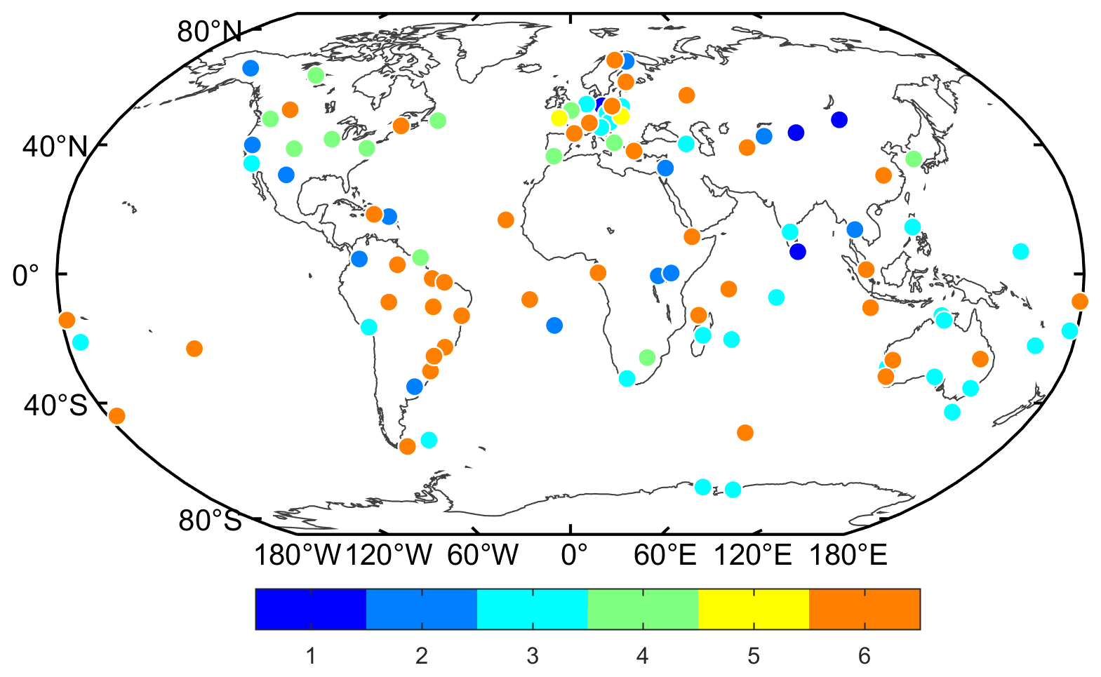
Figure 1Distribution of selected MGEX stations in January 2019. Six colors represent six different receiver types, which are listed in Table 1.
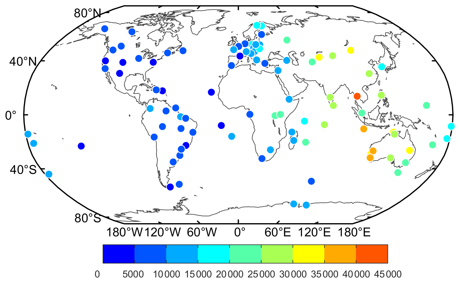
Figure 2Distribution of average number of available observation epochs for selected MGEX stations in January 2019.

The section begins by verifying the performance of the DCB estimation method, in which the satellite and receiver DCBs are compared with the DCB products by CAS and DLR. Then, the intraday stability of the receiver DCB is analyzed. The intraday stability of receiver DCB obtained by using BDS-2-only and BDS-3-only observations are finally compared.
3.1 Validation of DCB estimation method.
To verify the performance of the DCB estimation method, we take the DCB products from CAS and DLR as references, and we use the mean difference and rms values to evaluate the estimated satellite and receiver DCBs. Figure 3 shows the mean difference and rms of the estimated satellite DCB with respect to CAS and DLR values. It can be seen that the estimated satellite DCB shows a good agreement with CAS and DLR. The mean differences are mostly within ±0.2 ns, and their mean values with respect to DLR and CAS are −0.004 and −0.006 ns, respectively. The rms values are less than 0.4 ns, and the mean rms values with respect to DLR and CAS are 0.18 and 0.23 ns, respectively. It can be concluded that the DCB estimation method can obtain a satellite DCB that is in good agreement with DLR and CAS. In other words, it has little influence on the estimation result of satellite DCB when the receiver DCB is estimated epoch by epoch.

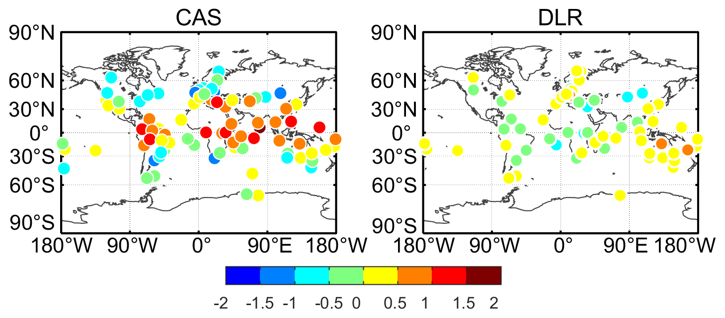
Figure 4The difference between the estimated BDS receiver DCB with respect to CAS and DLR.
Figures 4 and 5 present the mean difference and rms of the estimated BDS receiver DCB with respect to CAS and DLR values. It should be noted that the receiver DCB for some of our selected MGEX stations cannot be provided by CAS and DLR since these stations were not used in their DCB estimation. In this study, 101 station reference values can be provided by CAS and 61 station reference values can be provided by DLR. As it can be seen, when DLR is taken as a reference, the mean difference mostly ranges from −0.5 to 0.5 ns, and their mean value is 0.05 ns. The corresponding rms values are mostly less than 0.5 ns, and the mean rms is 0.43 ns. However, the difference between our estimated receiver DCB and CAS shows a larger value. The difference ranges from −2 to 2 ns; the values for some stations located in low latitudes are more than 1 ns. In terms of rms, the values for most stations are less than 1 ns, and the corresponding mean rms is 0.80 ns. The reason may be related to the single-station ionosphere modeling adopted by CAS, since the modeling accuracy of stations in low latitudes is low. The evaluation results show that the DCB estimation method can obtain the receiver DCB value with certain accuracy.

Figure 5The rms of estimated receiver DCB with respect to CAS and DLR.
3.2 Intraday stability of receiver DCB
In this study, the time series values of the receiver DCB within 1 d can be obtained through the epoch-by-epoch estimation for the receiver DCB. In order to better understand the intraday variations and stability of receiver DCB, we calculate and analyze the intraday standard deviation (iSD) and the intraday fluctuation as
where iSD is the intraday SD, RDCBi is the receiver DCB at epoch i, is the corresponding mean value of 1 d, N is the number of the available epochs, fDCBi is the corresponding value of fluctuation at epoch i, and RDCB1 is the receiver DCB at the first available epoch.
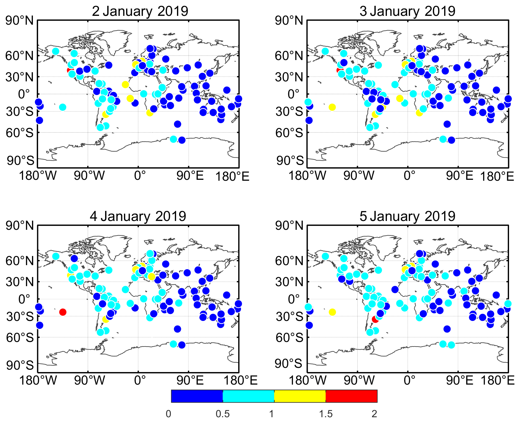
Figure 6The intraday SD of receiver DCB for all stations on 4 consecutive days (2, 3, 4, and 5 January 2019).
Four consecutive days (2, 3, 4, and 5 January 2019) are taken as an example. The intraday SD of receiver DCB for all stations on the 4 consecutive days is shown in Fig. 6, and the statistical results of intraday SD are listed in Table 2. As can be seen from Fig. 6, the intraday SD of receiver DCB for all stations shows similar values on 4 consecutive days. This result can also be shown in Table 2, with similar minimum, maximum, and mean values of intraday SD on the 4 consecutive days. It indicates that the intraday stability of the receiver DCB for most stations is almost the same on the 4 consecutive days.
Table 2Statistics of intraday SD of receiver DCB for all stations on 4 consecutive days.
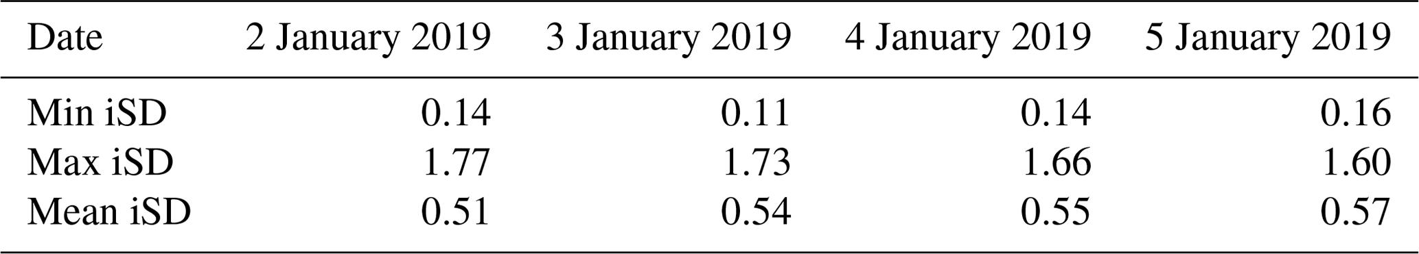
As can also be seen from Fig. 6, the intraday SD of the receiver DCB for most stations is less than 1 ns on the 4 consecutive days. In particular, the intraday SD of the receiver DCB for the stations located in the Asia Pacific region are significantly less than that for other regions. The reason may be related to greater quantities of available observations of these stations in the Asia Pacific region. In addition, some stations with larger intraday SD of the receiver DCB can be found in low-latitude regions, which may be related to the fact that the ionosphere is more active at low latitudes (Li et al., 2018). It can be concluded that the available observations of the station and the level of ionospheric activity of the area where the station is located may be two important factors affecting the intraday stability of the receiver DCB.
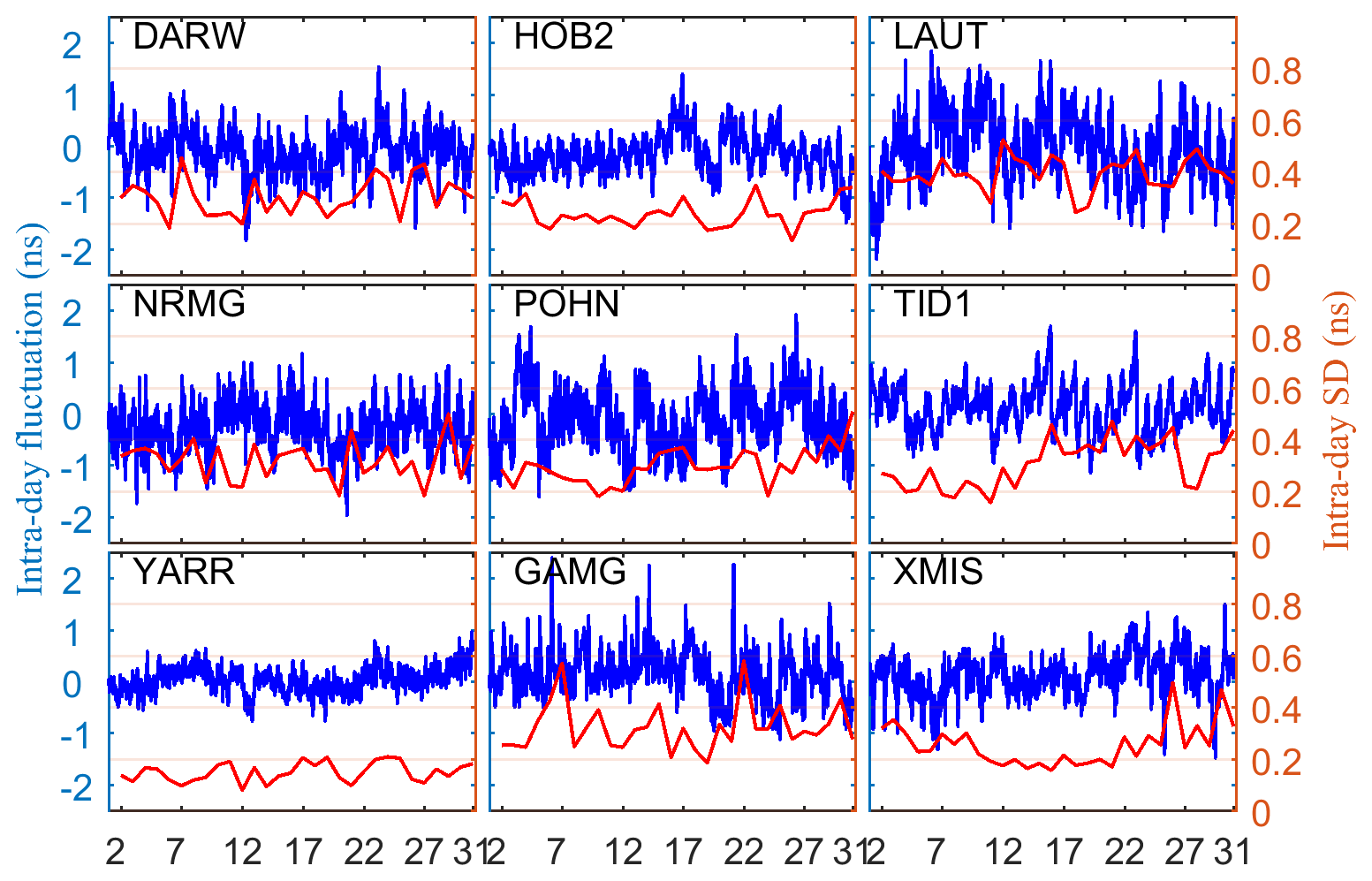
Figure 7The intraday fluctuation (blue line) and intraday SD (red line) of the receiver DCB for the nine selected stations within 30 d.
Figure 7 shows the intraday fluctuation and intraday SD of the receiver DCB for the nine selected stations located in the Asia Pacific region within 30 d. It can be seen that the intraday fluctuation of the receiver DCB is mostly within ±1 ns, and the corresponding intraday SD is mostly less than 0.4 ns. It is clear that the receiver DCB with larger fluctuation shows lower intraday stability and vice versa. Although intraday receiver DCB of the nine selected stations are relatively stable, larger fluctuations with more than 2 ns of intraday receiver DCB can be found.
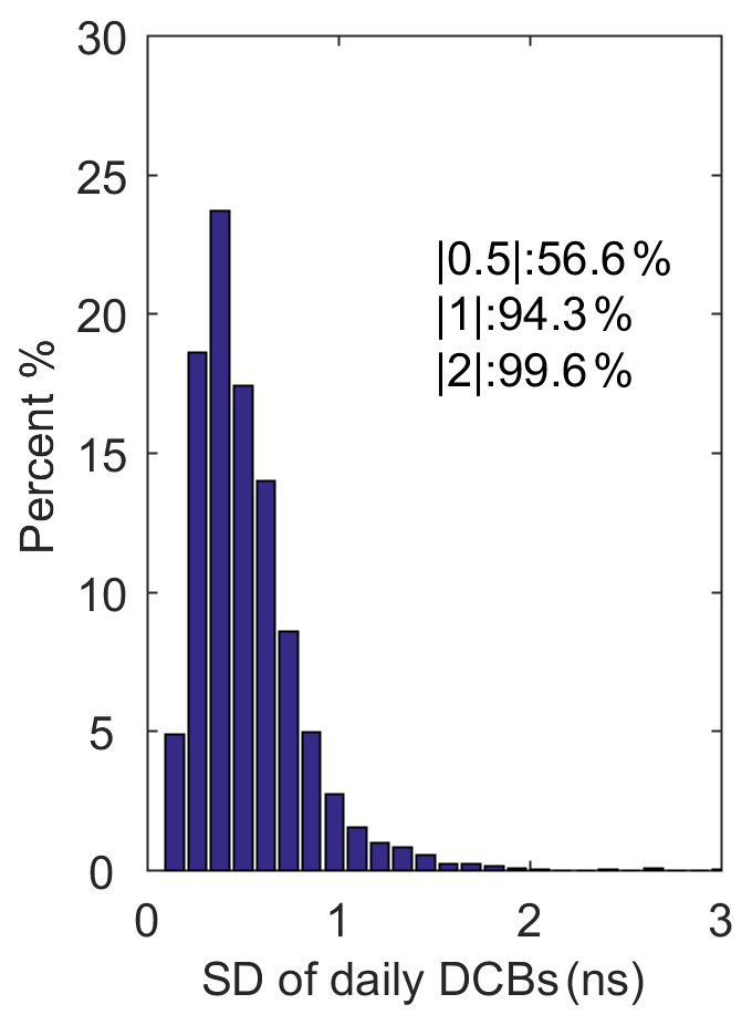
In order to better explain the intraday stability of the receiver DCB, Fig. 8 shows the statistical distribution of intraday SD of the receiver DCB for all stations on 30 d, where , , and represent the percentage of the absolute value of intraday SD is less than 0.5, 1, and 2 ns, respectively. More than 94 % of the intraday SDs are less than 1 ns, indicating that most of the receiver DCBs show relative stability within 1 d with the intraday SD of less than 1 ns.
3.3 Comparison between BDS-2-only and BDS-3-only solutions
As we all know, BDS-3 is the next-generation satellite navigation system. The additional BDS-3 observations used in this study contribute to the increasing available observables in DCB estimation. To further understand the contribution of BDS-3, we compare the intraday stability of the receiver DCB obtained by using BDS-2-only and BDS-3-only observations. Figures 9 and 10 show the mean intraday SD of receiver DCB and the corresponding statistical distribution for all stations within 30 d by using BDS-2-only and BDS-3-only observations. Obviously, the result shows that the intraday stability of the BDS-3 receiver DCB is better than that of the BDS-2 receiver DCB.
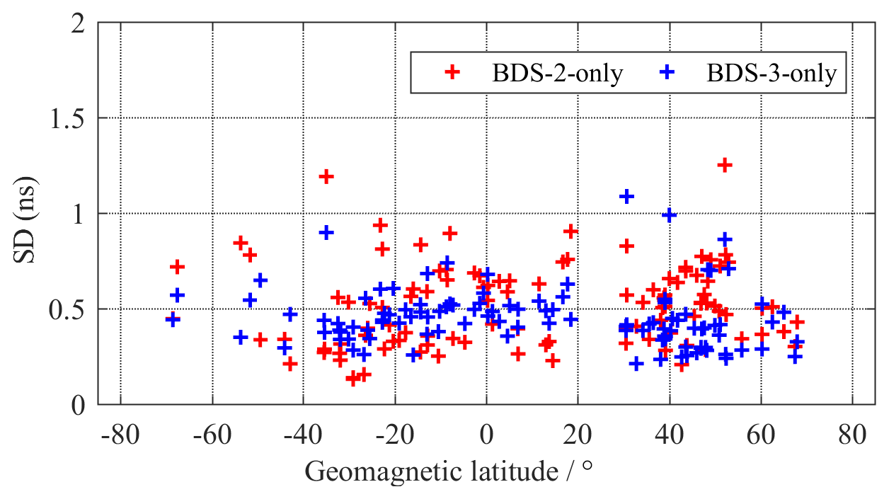
Figure 9The mean intraday SD of receiver DCB for all station in 30 d by using BDS-2-only and BDS-3-only observations.
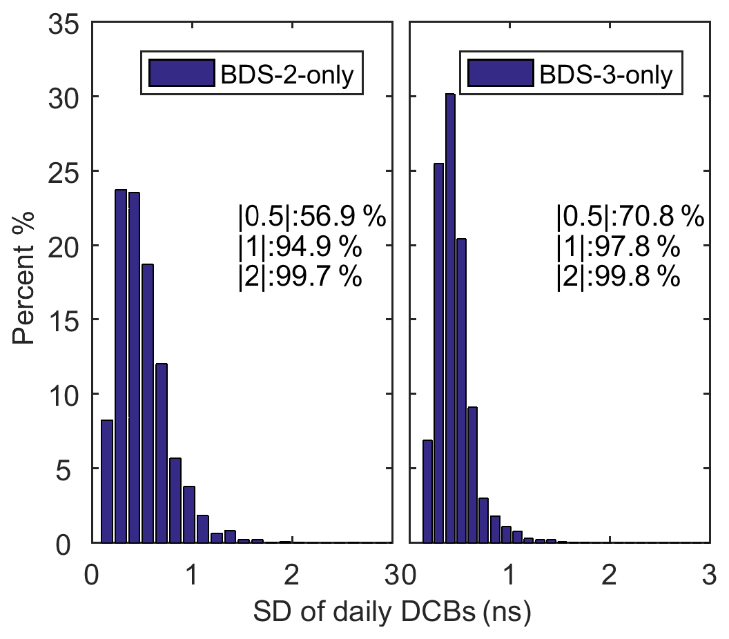
Figure 10Statistical distribution of intraday SD of receiver DCB by using BDS-2-only and BDS-3-only observations.
The short-term variations of epoch-by-epoch BDS receiver DCB are estimated and analyzed with additional BDS-3 observations. The BDS receiver DCBs with the additional BDS-3 observations are analyzed through 30 d of Multi-GNSS Experiment observations. To verify the performance of the DCB estimation method, we take the DCB products from CAS and DLR as references, and we use the mean difference and rms values to evaluate the estimated satellite and receiver DCBs. The estimated satellite DCB shows a good agreement with CAS and DLR, since the mean differences are mostly within ±0.2 ns, and their mean values with respect to DLR and CAS are −0.004 and −0.006 ns, respectively. The rms values are less than 0.4 ns, and the mean rms values with respect to DLR and CAS are 0.18 and 0.23 ns, respectively. In terms of the intraday variability of the receiver DCB, most of the receiver DCBs show relative stability within 1 d with the intraday SD of less than 1 ns. However, larger fluctuations with more than 2 ns of intraday receiver DCB can be found. It can be concluded that the available observations of the station and the level of ionospheric activity of the area where the station is located may be two important factors affecting the intraday stability of the receiver DCB. As shown by the results of the intraday stability of receiver DCB obtained by using BDS-2-only and BDS-3-only observations, the intraday stability of the BDS-3 receiver DCB is better than that of the BDS-2 receiver DCB.
The MGEX station data can be downloaded from ftp://cddis.gsfc.nasa.gov/pub/gps/data/ (Crustal Dynamics Data Information System, 2020).
QW carried out the analysis and wrote the paper. All co-authors helped in the interpretation of the results, read the paper, and commented on it.
The authors declare that they have no conflict of interest.
We thank IGS for providing MGEX data and DLR and CAS for providing the DCB products.
This research has been supported by the National Natural Science Foundation of China and the German Science Foundation (NSFC-DFG) project (grant no. 41761134092), the Startup Foundation for Introducing Talent of NUIST (grant no. 2243141801036), the Jiangsu Province Distinguished Professor Project (grant no. R2018T20), and the Open fund project of Hubei Research Center of Engineering and Technology for bridge safety monitoring and equipment (grant no. QLZX2014010).
This paper was edited by Steve Milan and reviewed by two anonymous referees.
Choi, B.-K. and Lee, S. J.: The influence of grounding on GPS receiver differential code biases, Advances Space Res., 62, 457–463, https://doi.org/10.1016/j.asr.2018.04.033, 2018.
Crustal Dynamics Data Information System, ftp://cddis.gsfc.nasa.gov/pub/gps/data/, last access: 20 May 2020.
Fan, L., Li, M., Wang, C., and Shi, C.: BeiDou satellite's differential code biases estimation based on uncombined precise point positioning with triple-frequency observable, Adv. Space Res., 59, 804–814, https://doi.org/10.1016/j.asr.2016.07.014, 2017.
Hernández-Pajares, M., Juan, J. M., and Sanz, J.: New approaches in global ionospheric determination using ground GPS data, J. Atmos. Sol.-Terr. Phy., 61, 1237–1247, 1999.
Hernández-Pajares, M., Juan, J., Sanz, J., Orus, R., Garcia-Rigo, A., Feltens, J., Komjathy, A., Schaer, S., and Krankowski, A.: The IGS VTEC maps: a reliable source of ionospheric information since 1998, J. Geodesy, 83, 263–275, 2009.
Hernández-Pajares, M., Roma-Dollase, D., Krankowski, A., García-Rigo, A., and Orús-Pérez, R.: Methodology and consistency of slant and vertical assessments for ionospheric electron content models, J. Geodesy, 91, 1–10, 2017.
Jin, R., Jin, S. G., and Feng, G. P.: M_DCB: Matlab code for estimating GNSS satellite and receiver differential code biases, Gps Solutions, 16, 541–548, https://doi.org/10.1007/s10291-012-0279-3, 2012.
Jin, S. G., Jin, R., and Li, D.: Assessment of BeiDou differential code bias variations from multi-GNSS network observations, Ann. Geophys., 34, 259–269, https://doi.org/10.5194/angeo-34-259-2016, 2016.
Jin, S. G. and Su, K.: PPP models and performances from single- to quad-frequency BDS observations, Satellite Navigation, 1, https://doi.org/10.1186/s43020-020-00014-y, 2020.
Li, M., Yuan, Y., Wang, N., Liu, T., and Chen, Y.: Estimation and analysis of the short-term variations of multi-GNSS receiver differential code biases using global ionosphere maps, J. Geodesy, 92, 889–903, https://doi.org/10.1007/s00190-017-1101-3, 2018.
Li, X., Xie, W., Huang, J., Ma, T., Zhang, X., and Yuan, Y.: Estimation and analysis of differential code biases for BDS3/BDS2 using iGMAS and MGEX observations, J. Geodesy, 93, 419—435, https://doi.org/10.1007/s00190-018-1170-y, 2019.
Li, Z., Yuan, Y., Li, H., Ou, J., and Huo, X.: Two-step method for the determination of the differential code biases of COMPASS satellites, J. Geodesy, 86, 1059–1076, https://doi.org/10.1007/s00190-012-0565-4, 2012.
Li, Z., Yuan, Y., Fan, L., Huo, X., and Hsu, H.: Determination of the Differential Code Bias for Current BDS Satellites, IEEE T. Geosci. Remote, 52, 3968–3979, https://doi.org/10.1109/tgrs.2013.2278545, 2014.
Liu, T., Zhang, B., Yuan, Y., Li, Z., and Wang, N.: Multi-GNSS triple-frequency differential code bias (DCB) determination with precise point positioning (PPP), J. Geodesy, 93, 765–784, https://doi.org/10.1007/s00190-018-1194-3, 2019.
McCaffrey, A. M., Jayachandran, P. T., Themens, D. R., and Langley, R. B.: GPS receiver code bias estimation: A comparison of two methods, Adv. Space Res., 59, 1984–1991, https://doi.org/10.1016/j.asr.2017.01.047, 2017.
Montenbruck, O., Hauschild, A., Steigenberger, P., Hugentobler, U., Teunissen, P., and Nakamura, S.: Initial assessment of the COMPASS/BeiDou-2 regional navigation satellite system, GPS Solutions, 17, 211–222, 2013.
Montenbruck, O., Hauschild, A., and Steigenberger, P.: Differential Code Bias Estimation using Multi-GNSS Observations and Global Ionosphere Maps, Navigation, 61, 191–201, https://doi.org/10.1002/navi.64, 2014.
Montenbruck, O., Steigenberger, P., Prange, L., Deng, Z., Zhao, Q., Perosanz, F., Romero, I., Noll, C., Stürze, A., and Weber, G.: The Multi-GNSS Experiment (MGEX) of the International GNSS Service (IGS) – achievements, prospects and challenges, Adv. Space Res., 59, 1671–1697, 2017.
Sanz, J., Juan, J. M., Rovira-Garcia, A., and González-Casado, G.: GPS differential code biases determination: methodology and analysis, GPS Solutions, 21, 1549–1561, 2017.
Schaer, S.: Mapping and predicting the Earth's ionosphere using the Global Positioning System, 59, Astronomical Institute, University of Berne, 1999.
Shi, C., Fan, L., Li, M., Liu, Z., Gu, S., Zhong, S., and Song, W.: An enhanced algorithm to estimate BDS satellite's differential code biases, J. Geodesy, 90, 161–177, https://doi.org/10.1007/s00190-015-0863-8, 2015.
Su, K. and Jin, S.: Triple-frequency carrier phase precise time and frequency transfer models for BDS-3, GPS Solutions, 23, 86, 2019.
Wang, N., Yuan, Y., Li, Z., Montenbruck, O., and Tan, B.: Determination of differential code biases with multi-GNSS observations, J. Geodesy, 90, 209–228, https://doi.org/10.1007/s00190-015-0867-4, 2016.
Wang, Q., Jin, S. G., Yuan, L., Hu, Y., Chen, J., and Guo, J.: Estimation and Analysis of BDS-3 Differential Code Biases from MGEX Observations, Remote Sensing, 12, 68, https://doi.org/10.3390/rs12010068, 2019.
Wellenhof, B. H., Lichtenegger, H., and Collins, J.: Global positioning system: theory and practice, Springer, ISBN 0387824774, 1992.
Xue, J., Song, S., and Zhu, W.: Estimation of differential code biases for Beidou navigation system using multi-GNSS observations: How stable are the differential satellite and receiver code biases?, J. Geodesy, 90, 309–321, https://doi.org/10.1007/s00190-015-0874-5, 2016.