the Creative Commons Attribution 4.0 License.
the Creative Commons Attribution 4.0 License.
 | 27 Jan 2020
Estimation of the westward auroral electrojet current using sparse magnetometer chain data
Marina A. Evdokimova
Anatoli A. Petrukovich
We investigate 1-D models of the westward substorm electrojet using magnetic field observations along a meridian chain of stations. We review two respective linear models from Kotikov et al. (1987) and Popov et al. (2001) with a large number of elementary currents at fixed positions. These models can be applied to a magnetometer chain with many magnetic stations. A new nonlinear method with one current element is designed for cases with a small number of stations. We illustrate the performance of these methods using data from the IMAGE (International Monitor for Auroral Geomagnetic Effects) and Yamal Peninsula stations. Several corrective measures are proposed to account for unphysical solutions or local extrema from the optimized functions. We also advertise a generic maximum likelihood approach to a problem that is feasible for any empiric model.
- Article
(3261 KB) - Full-text XML
- BibTeX
- EndNote


A ground-based magnetometer is the oldest instrument for space weather research. Data from hundreds of permanent and temporary magnetic stations all over the world are available. Using magnetic records, one can study evolution of the main geomagnetic field, as well as geomagnetic variations. Most of the latter are driven by the magnetospheric and ionospheric currents, which ultimately depend on solar activity. In particular, magnetic records are used to characterize the strength of geomagnetic substorms. The main substorm characteristic is the amplitude of magnetic variations in the northern auroral zone, which is summarized using the AE, AU, and AL geomagnetic indices. These variations are driven primarily by the westward auroral electrojet, which is an electric current that shortcuts the magnetotail cross-tail current (Ganushkina et al., 2018).
The goal of a dozen (about 12) AE/AU/AL stations is to catch the global maximum of magnetic perturbation at all longitudes. To study electrojet and substorm dynamics in detail, one needs to track at least one meridional profile of auroral geomagnetic variations with a north–south chain of stations. The most famous and accessible chains of stations are the Scandinavian IMAGE (International Monitor for Auroral Geomagnetic Effects) chain (Viljanen and Hakkinen, 1997), and the Canada/Alaska chains. Meridional electrojet profiles depend on the substorm phase and the strength of the solar wind driving. In the course of a substorm, the activity zone first shifts equatorward during growth phase, and then, after an onset, it retreats poleward. For stronger substorms, the auroral zone shifts equatorward (Feldstein and Starkov, 1967; Akasofu, 1968).
While the primary measured parameter is the magnetic field, it needs to be converted to electric current, which can then be compared with magnetospheric currents and used to quantify substorms as a plasma phenomenon. Alternatively, one can compute the geoelectric field, which affects pipelines or electric power lines. Ionospheric parameters in the auroral zone, such as electron density and conductivity, are also of interest (Untiedt and Baumjohann, 1993).
A number of quantitative and semiquantitative approaches have been developed to convert the magnetic field to electric current in the auroral zone. A 2-D model of equivalent ionospheric currents can be implemented if stations are distributed along both latitude and longitude (Amm and Viljanen, 1999). Several 1-D algorithms are also available. Kotikov et al. (1987) approximated an electrojet with a series of current wires that are evenly distributed at an altitude of 100 km. Popov et al. (2001) introduced an electrojet as a set of current strips with a fixed width at an altitude of 115 km. These models are described in detail in Sect. 2. Using a simpler approach, the Norwegian station network was utilized to define the boundaries of the auroral oval, tracking maxima of vertical magnetic component (Johnsen, 2013). Kamide et al. (1982) suggested a simple method to estimate the electric current density using just one station (given in the Appendix). By utilizing a statistical approach, the average oval boundaries can be related to the AL index (Starkov, 1994; Vorobjev et al., 2013). The Starkov (1994) model is provided in the Appendix. Note, however, that almost all oval models return the boundaries of auroral lights or precipitations, rather than the boundaries of auroral currents. More global models also exist that recover electric currents from a distributed set of stations (e.g., Mishin, 1990)
Most of these methods, which use instantaneous measurements, require a large number of stations to discover the electrojet spatial structure. However, in many local time sectors the station network is sparse. In this report, we develop a simple model of the westward electrojet and a relevant solution scheme, which can be used with a small number of stations (even with just two or three stations). We also describe some other useful algorithms. The key to our approach is the essential use of the vertical component of the geomagnetic field (z).
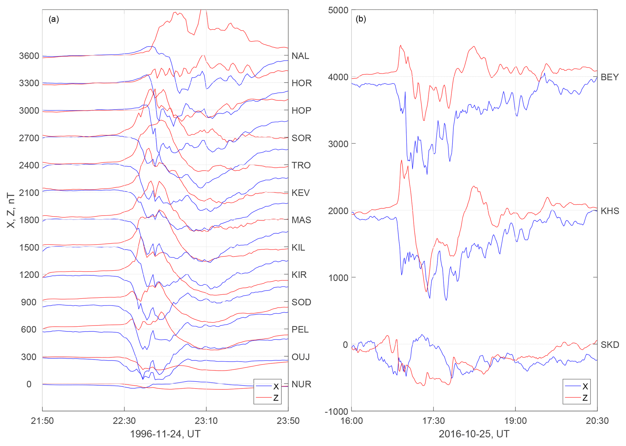
For illustration, we use two typical substorms with sudden onsets and clear negative bays that are gradually moving northward (Fig. 2). The first case was registered on 24 November 1996 by the IMAGE network and has been widely studied elsewhere (Petrukovich, 1999; Raeder et al., 2001; Slinker, 2001). The second case was recorded on the Yamal Peninsula (Papitashvili et al., 1985). The time resolution of the data is 1 min. Detailed information about the IMAGE network can be found at https://space.fmi.fi/image/www/, last access: 15 January 2020, and a map of the Yamal network is shown in Fig. 1. The station coordinates are given in Table 1.
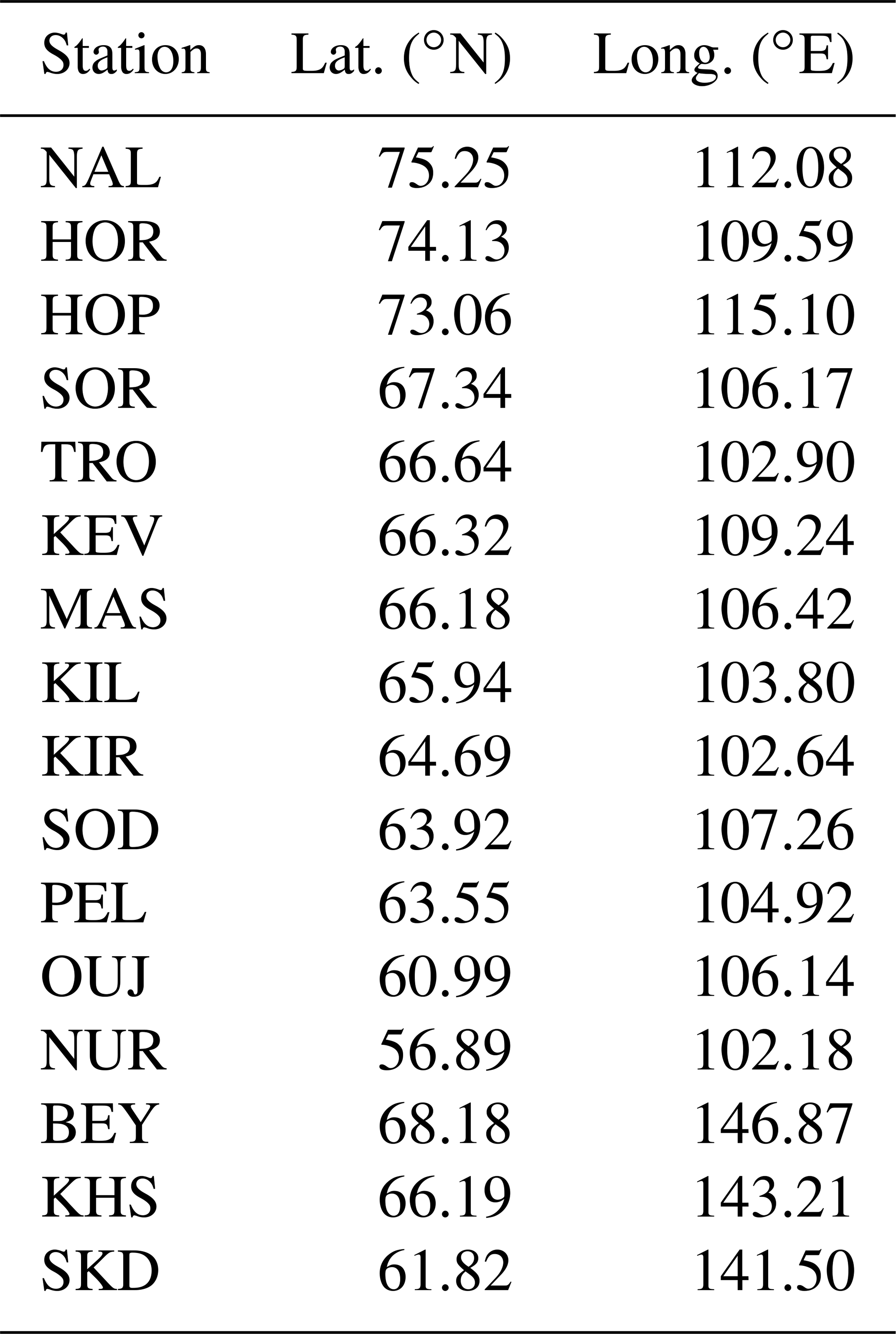
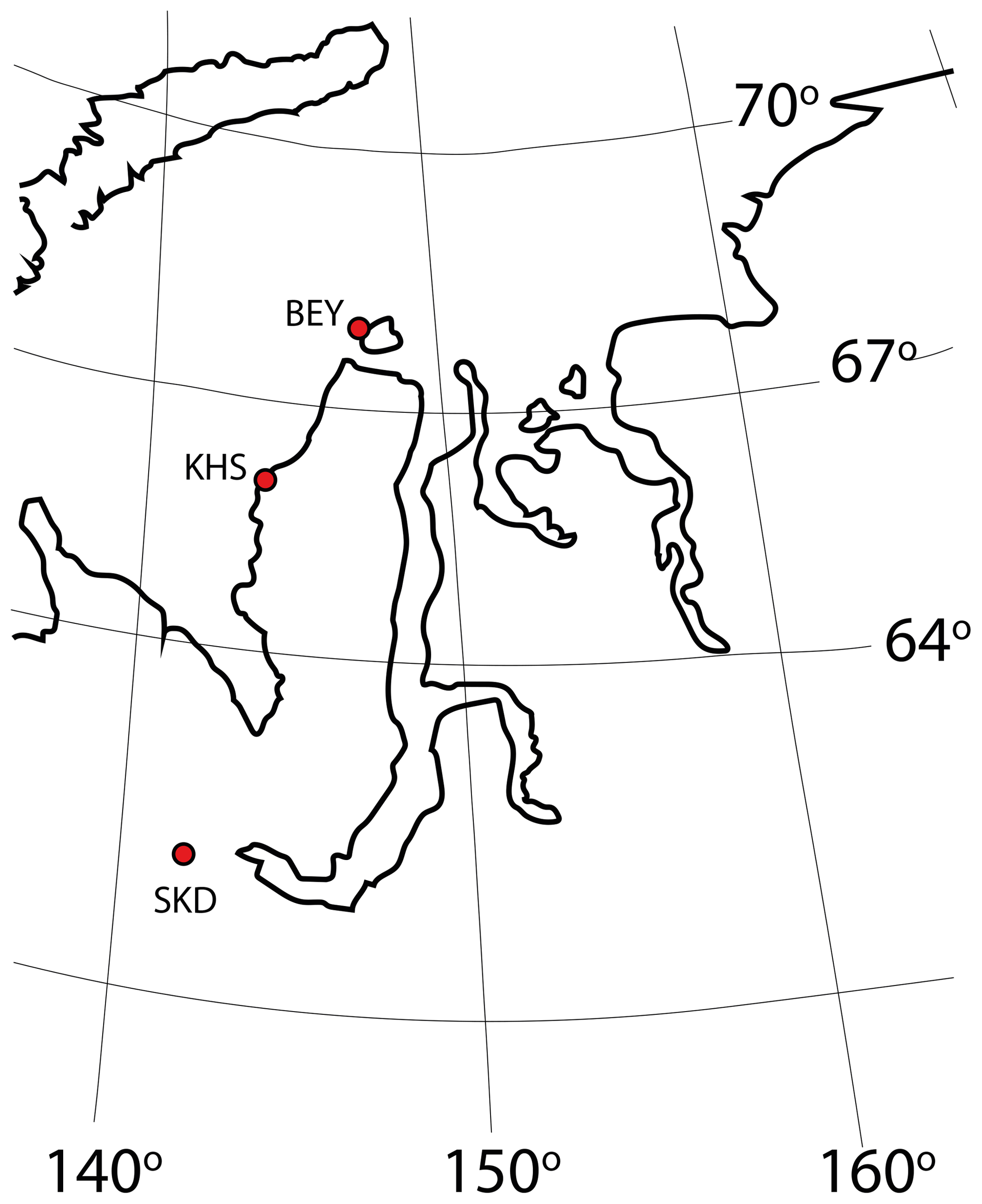
Figure 1Map of stations on the Yamal Peninsula.
2.1 General approach
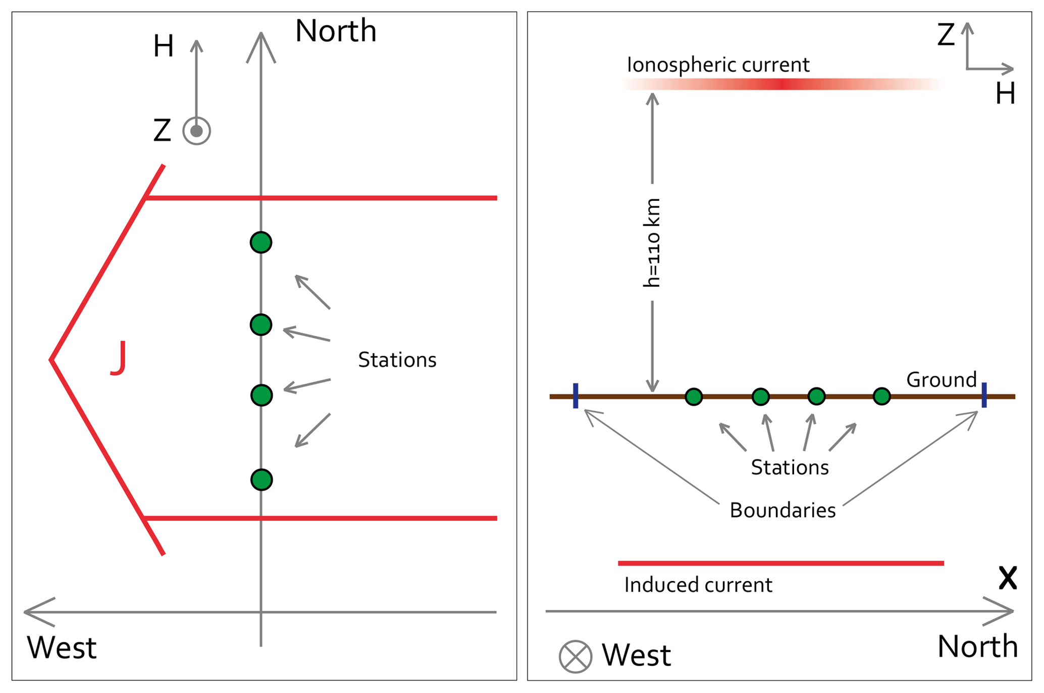
We use the following approximation of the 1-D westward auroral electrojet (Fig. 3): (1) the electrojet flows at a fixed altitude of 110 km above the flat land; (2) the electrojet is infinitely thin vertically; (3) the electrojet flows along in the latitudinal direction; and (4) the electrojet does not vary with longitude.
The magnetic disturbances in question are deviations from the quiet field, which has to be subtracted from the measurements. To determine the quiet level, we average magnetic data from the 5 quietest days of the month, during which the substorm occurred (Chapman and Bartels, 1940). The model latitudinal range spans ±4∘ from the southernmost and northernmost stations (for the models with many elementary currents). The input magnetic field disturbance is forced to be zero at the edges of this range in order to avoid nonphysical solutions. Ground magnetic disturbances are produced by the ionospheric current (electrojet) and the corresponding induction current inside the Earth. The model latitudinal profile of ionospheric current is reconstructed using the north–south X and the vertical Z magnetic components that are measured at a set of ground observatories (magnetic stations). Currently, we ignore the Y component of the magnetic field.
2.2 Separation of external and internal field components
Ground magnetic disturbances can be described as
where the “e” and “i” indices denote external and internal components, respectively. According to Pudovkin (1960), the difference between the external and internal components at any point x along meridian can be calculated as follows (here H is horizontal field component):
Therefore, the external field components are
This method works well for a dense magnetometer chain with a large number of stations. H(ξ) and Z(ξ) are obtained using the linear or spline interpolation of the measured magnetic disturbance (forced to zero at the edges of the modeled latitudinal range; see previous subsection). Integrals are calculated over the same latitudinal range.
For magnetometer chains with a small number of stations, we have to use the simpler method (Petrov, 1982) that has constant, empirically justified coefficients:
2.3 Solution scheme
We formulate the general maximum likelihood estimation (MLE) solution. We choose the model parameters that maximize the likelihood function L:
where N is the number of stations; Xk and Zk represent the disturbance of the magnetic field, caused by the electrojet current, measured at the station k (with the background field and induction field subtracted); Pk is the probability of observing the given magnetic fields Xk and Zk for an electrojet model with the parameter vector p; and Pp represents a priori probabilities for p.
A priori information (also referred to as “priors”) may be predictions from the statistical models or common sense limitations, such as the flatness of the spatial profile. The latter variant is also known as regularization. Regularization might be technically necessary for under-determined problems, when the number of free parameters is larger than the number of degrees of freedom in the sample (the number of independent measurements).
In this investigation, we use one of the simplest MLE variants, assuming a Gaussian distribution of the model residuals and solving the general OLS (ordinary least squares) inverse problem.
where n is the model number, and are calculated model disturbances, Qr denotes possible additional constraints, and σX (σZ) represents standard variations of the measured X (Z) components (at all stations used at a given time).
The parameter vector is determined by looking for the minimum of −2ln L. If the whole model is linear with respect to the parameter vector p, the standard matrix inversion technique is applied to acquire the solution. The nonlinear variants are solved here using the Levenberg–Marquardt algorithm. This method requires the specification of some initial values of the model parameters, and then moves along the gradient of the optimization function towards the minimum. Unlike linear regression, methods such as these for nonlinear problems do not guarantee a unique solution due to existence of local minima.
The errors of the model parameters p are calculated as the inverted Hessian of ln L:
2.4 Model 1
The first model described was suggested by Kotikov et al. (1987). It includes a large number of the infinitely thin, fixed wires with unknown currents. The wires are evenly distributed within the modeled latitudinal range, which is from the stations closest to the Equator and the pole-most stations. The magnetic field at the edge wires is set to zero.
Here, h is the height of the wires, M is the number of the wires, Ij represents currents, and j=1…M and are the difference in the coordinates of the wire j and the station k along the magnetic meridian, respectively. The model magnetic disturbances and depend on the unknown model parameters Ij in a linear fashion.
Regularization, suggested by the authors, is
where Iaj is the current at the previous time step; coefficient α does not allow currents to change too quickly (controls smoothness in the time domain), and q controls smoothness of the current profile along the meridian. Regularization is necessary, as the number of wires (of the model parameters) can be larger than the number of stations (50 wires were proposed in the original paper). Still, the number of stations should be large enough (e.g., as in the IMAGE chain) to provide enough information on the spatial inhomogeneity of the current.
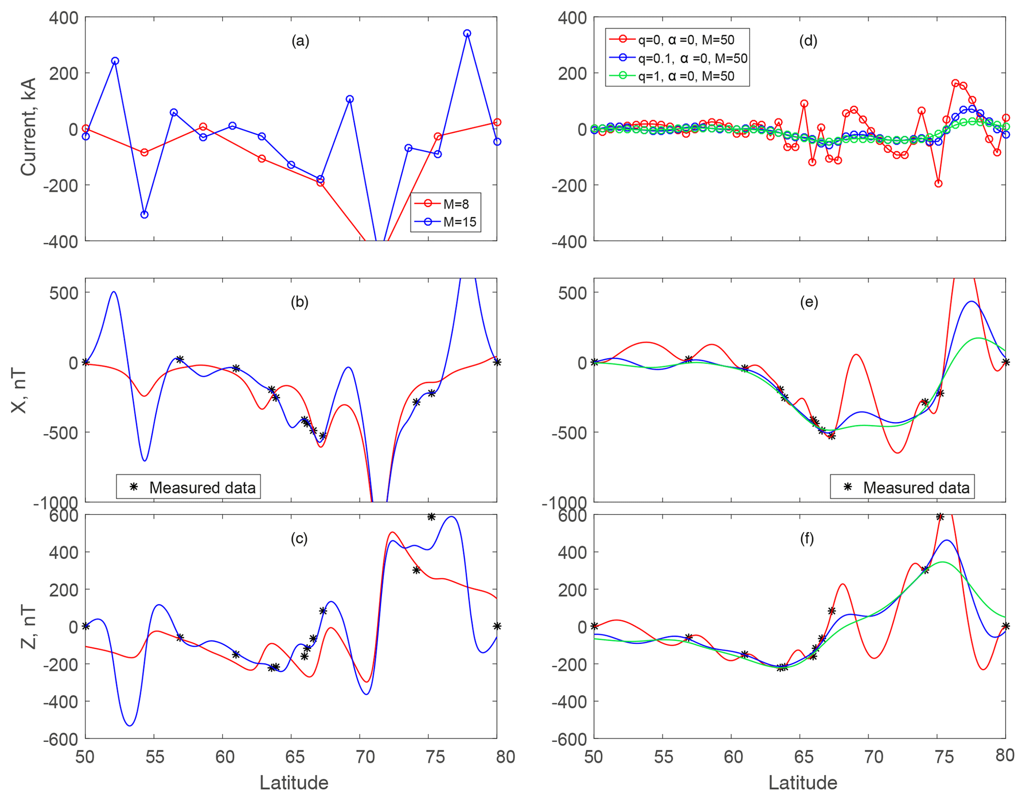
Figure 4Event on 24 November 1996 at 23:09:00 UT. (a, b, c) Model 1 with 8 and 15 wires with no regularization. (d, e, f) Model 1 with 50 wires with and without regularization. The measured field is shown using black stars, and the model field and current are shown using lines.
2.5 Model 2
The second model described was suggested by Popov et al. (2001). It is fundamentally similar to Model 1, except it consists of evenly distributed strips with an unknown current density.
where d is the half-width of the strip, and is the difference in coordinates of the strip center j and the station k. The positions of the strips are fixed. Disturbances and depend on the unknown model parameters ji in a linear fashion.
Regularization, suggested by the authors, is
Here, the coefficient q is responsible for the smoothness of the current profile along the latitude, and β limits the maximal current amplitude. Regularization is necessary, as a large number of strips is proposed in the original paper.
2.6 Model 3
For a small number of stations, a simpler model with one electric current element is required. Model 1 is inconvenient, as a single infinitely thin current will return an unphysical magnetic profile. We use a version of Model 2 that has one current strip with floating borders. The optimal unknown model parameters are as follows: the current density and the low-latitude and high-latitude electrojet boundaries (explained in the following section). This model is nonlinear.
Here, j is the current density in a strip; xh and xl are coordinates of the high-latitude and the low-latitude current borders, respectively; and xk is the coordinate of the station k.
3.1 Number of wires and regularization
In Model 1, each infinitely thin wire creates a characteristic spatial peak of the magnetic field with a latitudinal scale approximately equal to the height of the wire. As height (∼100 km or ∼1∘ of latitude) is much smaller than the typical electrojet width and the modeled latitudinal domain, a small set of wires will generate an unphysical magnetic profile with several sharp minima (for the westward electrojet). Figure 4a, b, and c present such Model 1 runs, using Example 1 with 8 and 15 wires (with no regularization). Both variants return oscillating magnetic profiles, indicating that the number of wires is insufficient. Note that the case with 15 wires also exhibits another problem, which is typical for models with too many parameters: some wires are attributed positive currents, creating positive excursions of the magnetic field between stations, which are not supported by any evidence (measured field).
The linear model with 15 wires becomes underdetermined, as the number of independent inputs (the double number of stations) is comparable to or smaller than the number of unknowns. An underdetermined solution usually results in physically unrealistic, large, and very variable values of (here) elementary currents that ideally cancel each other out at the magnetic stations, where measurements are available (Fig. 4d, e, and f; the model with 50 wires, red curves).
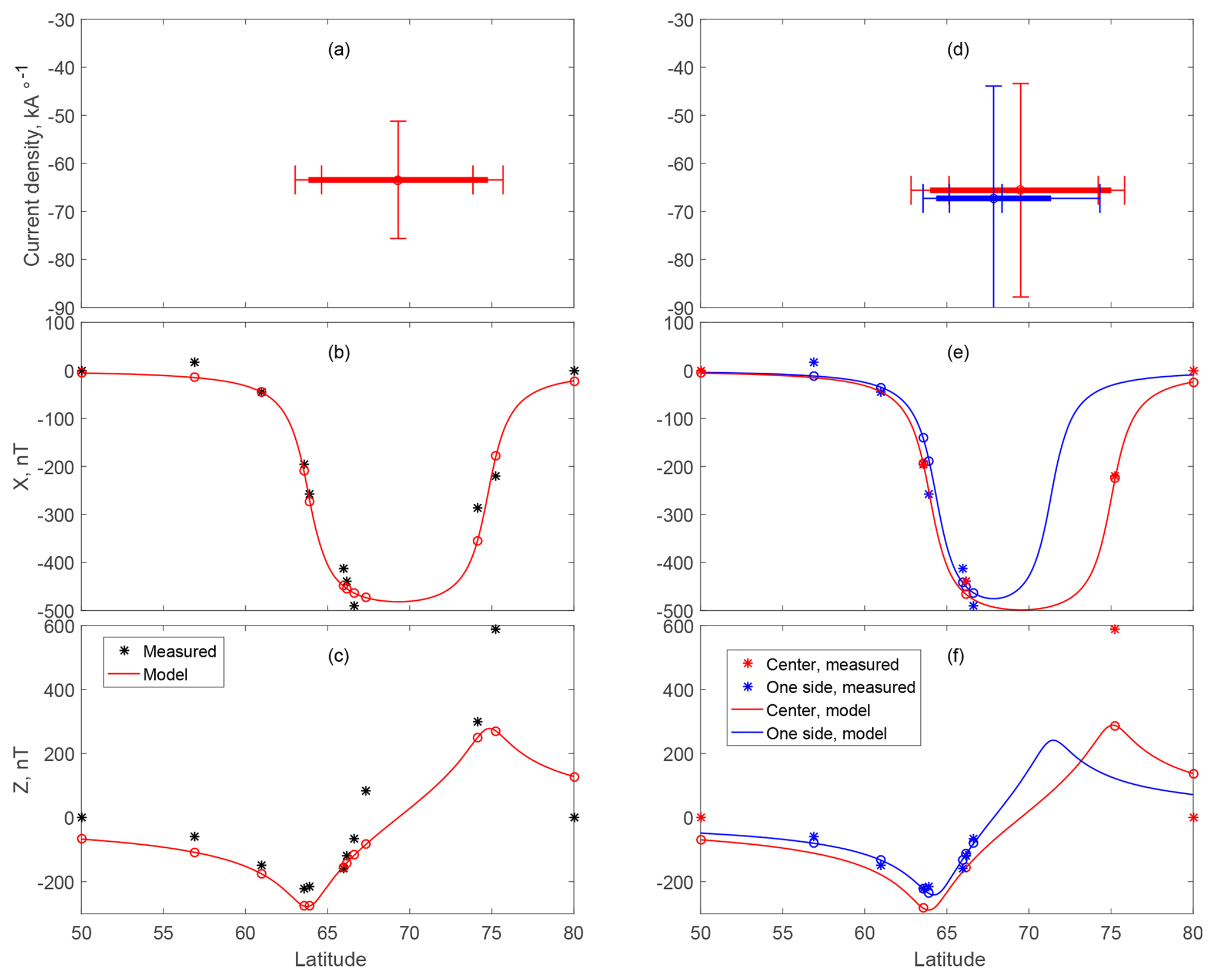
Figure 5Event on 24 November 1996 at 23:09:00 UT. Effect of the station selection. Panels (a, b, c) show many stations covering both boundaries of the electrojet. Panels (d, e, f) show a small number of stations on both sides of the electrojet (red) and near only one boundary (blue). The error bars (standard deviation) are shown using the thin lines in panels (a) and (d).
To ensure a sufficiently flat electrojet profile, a denser current network with the separation much smaller than the height is required; however, overly sharp variations between stations need to be damped. The standard way to solve this problem is to use the so-called regularization procedure, which penalizes variability and/or amplitude of the model parameters. The introduction of the regularization term in Model 1 with a reasonable coefficient q∼1 effectively reduces unwanted variations of currents, while still preserving reasonable complexity of the latitudinal profile (Fig. 4d, e, and f; the green curve compared with the blue and red curves).
Here, as seen in Fig. 4, it is important to note several aspects related to the applicability of such 1-D models. First, Model 1 reconstructs the X component reasonably well: the calculated values of the fields in Fig. 4d, e, and f always correspond to the measured data (black stars). However, the flattened Model 1 (with regularization) often fails to reproduce extreme Z values (such as at a latitude of 75∘).
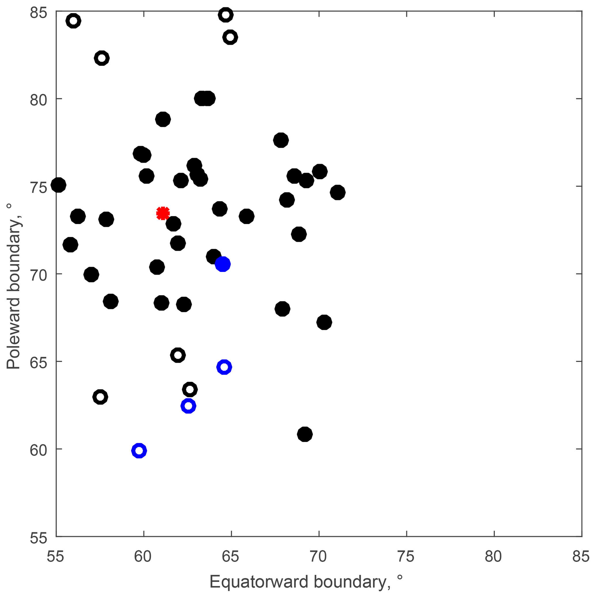
Figure 6Event on 24 November 1996 at 23:09:00 UT. The map of the initial conditions and the final electrojet boundaries for the case in Fig. 5d, e, and f (blue curve). The initial conditions are shown using black circles, the Starkov model (a center of randomized initials) is shown using the red point, the absolute minimum is shown using the blue filled circle, and the local minima are shown using blue open circles. See the text for further details.
Second, when the station coverage is sparse (which for IMAGE is in the Norwegian/Barents Sea – with stations only on the mainland and Svalbard), even the model with sufficient regularization may return positive currents (Fig. 4d, e, and f, above 75∘, green curve). This positive current results in positive model X values in the gaps between stations. However, all available stations only measure negative X; thus, the presence of a positive current cannot be directly confirmed. These issues are further elaborated upon in Sect. 5. With many elementary electric currents, it is possible to describe a relatively complex spatial profile of an electrojet without the need to explicitly define the nonlinear latitudinal profile. Elementary currents can be placed at evenly spaced fixed positions; thus, the only free model parameters are the electric current amplitudes in the numerator of the functional form (Eq. 8), and the model therefore remains linear. The spatial inhomogeneity of an electrojet is well described by these changing amplitudes.
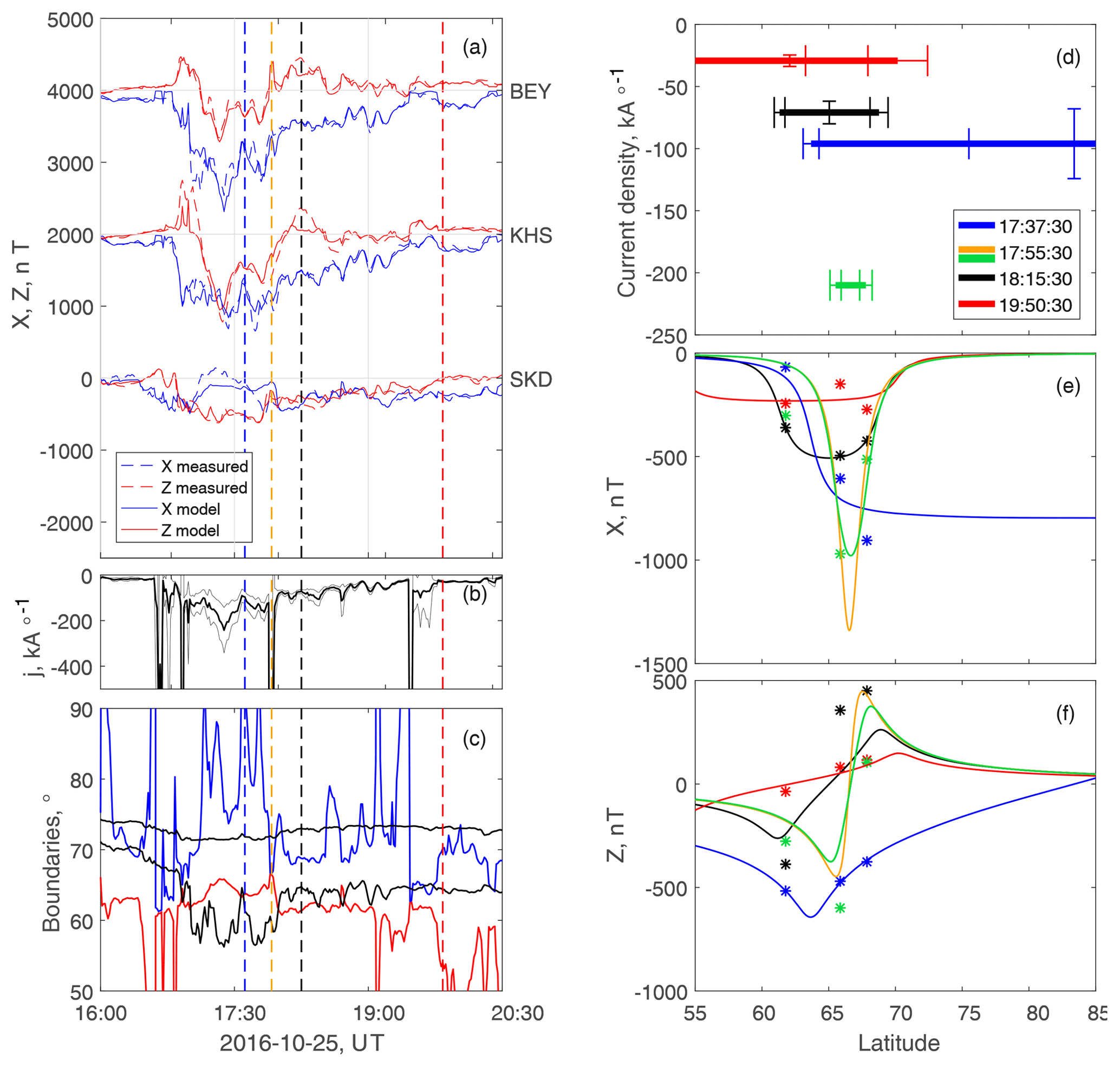
Figure 7Model 3 for Example 2. Panels (a, b, c) show the measured and magnetic time profiles, the model current density (the standard deviation range is given using thin curves), and the electrojet boundaries (black refers to the Starkov, 1994 model, and blue and red refer to Model 3). Vertical lines denote the time instants for the panels (d, e, f). Panels (d, e, f) show the latitude cuts with model parameters for four time instants. The error bars in panel (d) show the standard deviations. The measured field is shown using stars, and the model field is shown using lines. Orange illustrates the physically incorrect case which was removed using an additional physical consideration – the current density was forced to be equal to the estimate from Kamide et al. (1982) (see Sect. 3.4 and Appendix B in this paper). The corrected solution is shown using a green line.
3.2 Selection of parameters of the nonlinear model
The most natural variant for a case with a small number of stations is to use one strip from Model 2. The free parameters are then current density, center, and the half-width of the strip. However, this variant has several drawbacks.
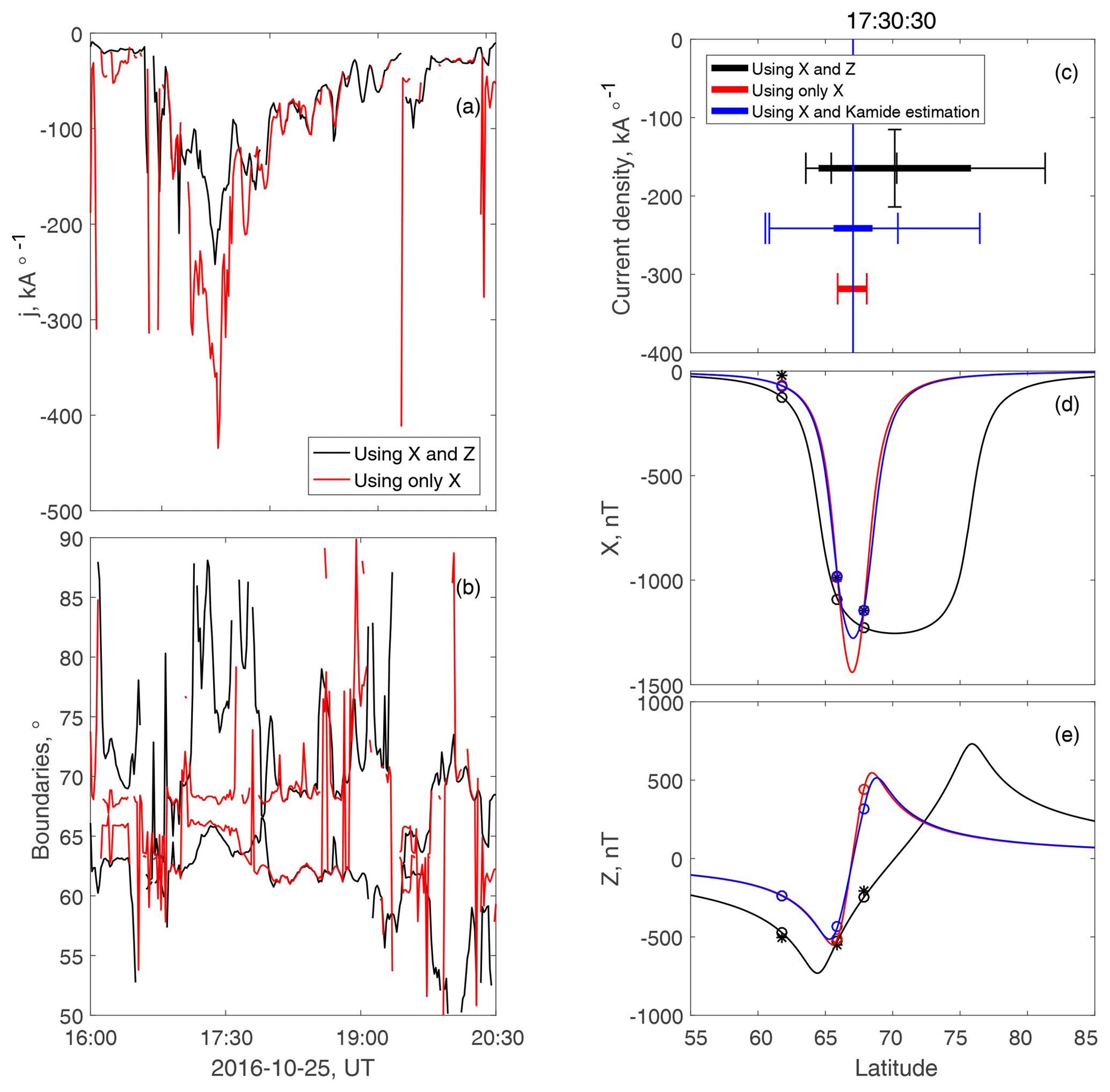
Figure 8Variants of Model 3 for Example 2. Panels (a, b) show the model current density and the electrojet boundaries (black shows the full Model 3 with X and Z inputs, and red shows the reduced Model 3 with only the X input). Panels (c, d, e) show the latitude cut for 17:30:30 UT for the two model variants and also for a variant with the current density fixed using the estimate from Kamide et al. (1982). The measured field is shown using black stars, and the model field and current are shown using lines. The error bars in panel (c) show the standard deviations.
The current density and width of the electrojet are strongly anticorrelated in the model with one strip and two to three magnetic stations. Almost the same magnetic field can be produced with a variety of strips with a different width and current density, but the same total current. The correlation of parameters complicates the error analysis, as the standard error bars are produced by the diagonal elements of the error matrix (Eq. 7). The correlation of the parameters creates large non-diagonal elements, which often avoid sufficient attention.
The second drawback is related to the definition of electrojet boundaries. For example, if there is no station in a relevant position to catch a poleward boundary, the corresponding error will be propagated to both parameters: the electrojet center and width.
Thus the optimal Model 3 has three parameters: the current density, and the poleward and equatorward boundaries. All parameters are defined almost independently. The current density mostly depends on the largest observed X component disturbance, and the boundaries depend on the sign of the Z component at the nearest station.
When the number of stations is small, the stations might quite often not be optimally located relative to a specific electrojet. To illustrate how this problem is handled using Model 3, we resurrect one latitudinal profile from Example 1 (Fig. 5). Figure 5a, b, and c show the model for the case with all stations, whereas the right panels show two variants. The red curve corresponds to the case with three stations, two southward and one northward electrojet, and the model electrojet is identical to that in the left panel (only the current density error is larger). However, the case with four stations (blue curve), all equatorward of the electrojet, results in a substantially different model with a shifted poleward border. This border is also defined with a substantially larger error. To get this particular solution, the local minimum must also be avoided; this issue is described in the next subsection.
3.3 Avoiding local minima
Contrary to with linear regression, the determination of the right nonlinear solution is not guaranteed. All algorithms are sequential and may lead to a local, rather than a global, minimum of the target function (Eqs. 5, 6). The result may depend on the initial approximation of the model parameters, which needs to be specified to start the search. There are several standard ways to avoid local minima in a more or less automatic fashion.
The first approach is to introduce a prior – some a priori information on the location of the electrojet boundaries or electrojet amplitude. The a priori boundaries can be taken, e.g., from the Starkov model (Starkov, 1994, shown in Appendix A of this paper). As an input for Starkov model one can take either the AL index or the local maximal negative X component (from the modeled magnetic chain data). In Eq. (6), one may then define , where d is a parameter, d0 is an a priori value, and wd is a weight. This form penalizes any strong deviations from the a priori value. Thinking about a solution process as a descent along the local gradient in a landscape of the minimized function, the introduction of a prior modifies this landscape, removing the local minima. However, although effective in some cases, this approach is very sensitive to the selection of weights, which have to be specified manually for each model run.
The second approach is to use a so-called multi-start algorithm. We generate a normally randomized set of initial conditions around a Starkov model solution, run Model 3 several times, and choose a result with the minimal residuals (Eq. 6). We show the map of 50 initial conditions (for the boundary locations only) in Fig. 6 for the case of Fig. 5 (c, d, e, blue curve). In Fig. 6, the Starkov model is shown using the red point, and the solutions (starting from the filled black circles) lead to the absolute minimum (shown using the filled blue point). The empty black circles lead to the local minima (blue open circles). As Model 3 is computationally simple, the method works well, and it is not necessary to densely fill the parameter space during randomization.
3.4 Model 3 test and the false global minimum problem
We illustrate the operation of Model 3 by running it for the whole of Event 2 (Fig. 7). In Fig. 7a, b, and c, the time profiles of the magnetic field, current density and electrojet boundaries are shown, respectively. This was a rather strong substorm with a negative bay of almost −1000 nT. Generally, Model 3 returns reasonable results for magnetic profiles (Fig. 7a), but the electrojet boundaries are somewhat different from the statistical Starkov model (Fig. 7c). During the growth phase (16:00–16:45 UT) the real electrojet is more poleward, which may be related to the absence of a station at a sufficiently southward location. During the extended recovery phase (after 18:00 UT), the electrojet is consistently more southward. However, a detailed analysis of this substorm is beyond the scope of this report.
Besides these easily interpretable results, at some moments the model reports definitely unphysical electrojet parameters, which appear as spikes in Fig. 7b and c. We highlight the four time instants with problems of various kinds (shown using colored vertical lines). The detailed model results for these instants are shown in Fig. 7d, e, and f.
The black vertical line (at 18:15:30 UT in Fig. 7a, b, and c) and the corresponding black curves (Fig. 7d, e, f) show fully reliable result with small errors. The blue lines and curves for 17:37:30 UT show the case with an unreliable poleward border, which is even above 90∘. Here, all three stations fall on the more equatorward side of the electrojet (all Z values are negative). The uncertainty interval for the poleward border is very large and extends down to a very reasonable latitude of 75∘. The corresponding equatorward border and current density are well defined, as expected. A similar error, but for the equatorward border, occurs at 19:50:30 UT (red color). Here all three stations have a positive Z.
A more serious problem arises if all three model parameters are physically incorrect, which is the case at 17:55:30 UT (orange). Here the model returns an electrojet with a zero width and a very high current density amplitude. The model X component profile shows a very narrow dip between the stations with an amplitude 1.5 times larger than the actual observed field (green stars). The model current density amplitude is very large and is therefore not shown.
The problems described are features of the true global maximum in the mathematical solution and cannot be resolved within the core model algorithm. They have to be removed using some additional physical considerations. In a case with one unreliable border, one can fix the troubled parameter at limiting values, e.g., 55 and 85∘; however, these numbers are not still justified by any observations.
Somewhat counterintuitively, the situation is simpler for an infinitely thin electrojet. One can force the current density to be equal to the estimate from Kamide et al. (1982) (see Appendix B). The model then returns a more reasonable, but still rather narrow (2∘ wide), electrojet (Fig. 7, green line). The green model in Fig. 7d corresponds to this adjusted solution. A substantial X value at the station closest to the Equator at 62∘ still suggests that the real electrojet is wider than the result, but the solution here balances both the X and Z residuals.
The optimal method to compute electrojet parameters using Model 3 and small number of stations is summarized below.
-
Select a substorm interval of interest, preferably with a clear westward electrojet.
-
Subtract the quiet magnetic field.
-
Subtract the internal component of the magnetic field using constant coefficients (Eq. 4).
-
Repeat the following actions for all time instants with 1 min or 5 min cadence.
-
Create a set of initial latitudes that are normally distributed around the boundaries of the Starkov (1994) model. The initial current density can be taken as equal to the estimate from Kamide et al. (1982) or randomized.
-
For each set of initial conditions, solve the minimization problem (Eqs. 6, 7, 12). The solution with the smallest residuals is final.
-
Check the values of parameters and errors to determine the reliability of individual parameters. If necessary, repeat the computation of the reduced model with a fixed current density, using the estimate of Kamide et al. (1982).
The proposed 1-D algorithms are computationally simple and efficiently recover the auroral electrojet parameters in configurations such as that of the westward electrojet developing during the substorm expansion phase. The possibility of only using a few magnetic stations substantially increases the span of longitudes at which such modeling is possible. The electrojet amplitude and location determined can be used for a variety of studies, including, for example, the comparison of electrojet boundaries with the oval boundaries, the comparison of electrojet amplitude with that registered in space using AMPERE project data (Anderson et al., 2000), or with magnetospheric modeling. It is potentially interesting to develop some extended auroral electrojet index with the SuperMAG dataset (Gjerloev, 2009), including electrojet total strength and location. Finally, the technique developed can be used to recover storm-time electrojets, which move to lower latitudes with sparser station coverage.
To be fully confident in the reconstructed meridional profile of the electrojet, one needs the station set to be dense enough at all of the latitudes in question. A 5∘ gap in the IMAGE chain in the ocean often appears to be too large for such a model. The 1∘ step, which is approximately equal to the electrojet height, is definitely sufficient. By also assuming a minimal electrojet width (e.g., 2∘), one can allow the equivalent couple of degree step. To capture only three electrojet parameters (the magnitude and the borders, Model 3), the stations need to be somewhat offset on both sides with respect to the actual electrojet location.
The models described have some natural physical limitations. First of all, any deviations from 1-D are effectively averaged out. Some issues, such as the deflection from the latitudinal direction, can be handled by the reasonable complication of the model (including the Y component in consideration). Model 3 can also be modified to use a bell-shaped electrojet profile. This variant may potentially decrease the effects of unphysically sharp electrojet edges. It is also reasonable to increase averaging by switching to a 5 min step.
It should be specially noted that the analysis of our test data reveals frequent apparent inconsistency between the X and Z magnetic components in 1-D approximation. Visually it can be identified as “overly large” Z excursions, which are comparable with the expected X values. In a gap with respect to station locations, models 1 and 2, taking such Z values into account, may generate unreasonable electrojet latitudinal profiles, including reverse currents, which are not supported by any observable positive X excursion. In Model 3 such Z values may result in deviations of the electrojet borders. Beyond the limits of the 1-D model, such Z excursions may be attributed to coastal effects or some vortex-like 2-D structures. Potentially, smaller confidence in Z can be accounted for in the model (Eq. 6) by attributing smaller weight to residuals in Z, e.g., with the coefficient 0.5. However, such an approach requires further statistical justification.
The usage of Z is inevitable in our case when the number of stations is small. In Fig. 8, we illustrate the alternative reduced Model 3 run for the event from Fig. 7, which does not take the Z component into account. The substantial difference only appears at 18:00–19:00 UT during the substorm expansion phase, when the reduced model reports a much narrower electrojet with a higher current density. A 2 to 3∘ wide electrojet in such condition is definitely unphysical. The investigation of Fig. 8e shows that proper knowledge of Z is essential to calculate the actual electrojet location.
Finally, we solve the considered mathematical problem with a very generic maximum likelihood approach, which allows priors, regularization, comprehensive error-handling, etc. This approach can be used in a variety of other empirical model studies.
In this study, we investigated the models of the westward auroral electrojet using magnetic field observations from sparse meridian chains of ground-based magnetometers. The model with one current strip works reasonably well, even using only three stations and two magnetic field components (X and Z). Some corrective actions proved to be necessary to avoid general computational problems related to unphysical minima in the nonlinear optimization algorithm. However, the model naturally cannot reliably estimate the location of the electrojet boundary when there are a lack of stations near that boundary. Special attention also needs to be paid in future to reconciliating the contradictory profiles of the X and Z magnetic components.
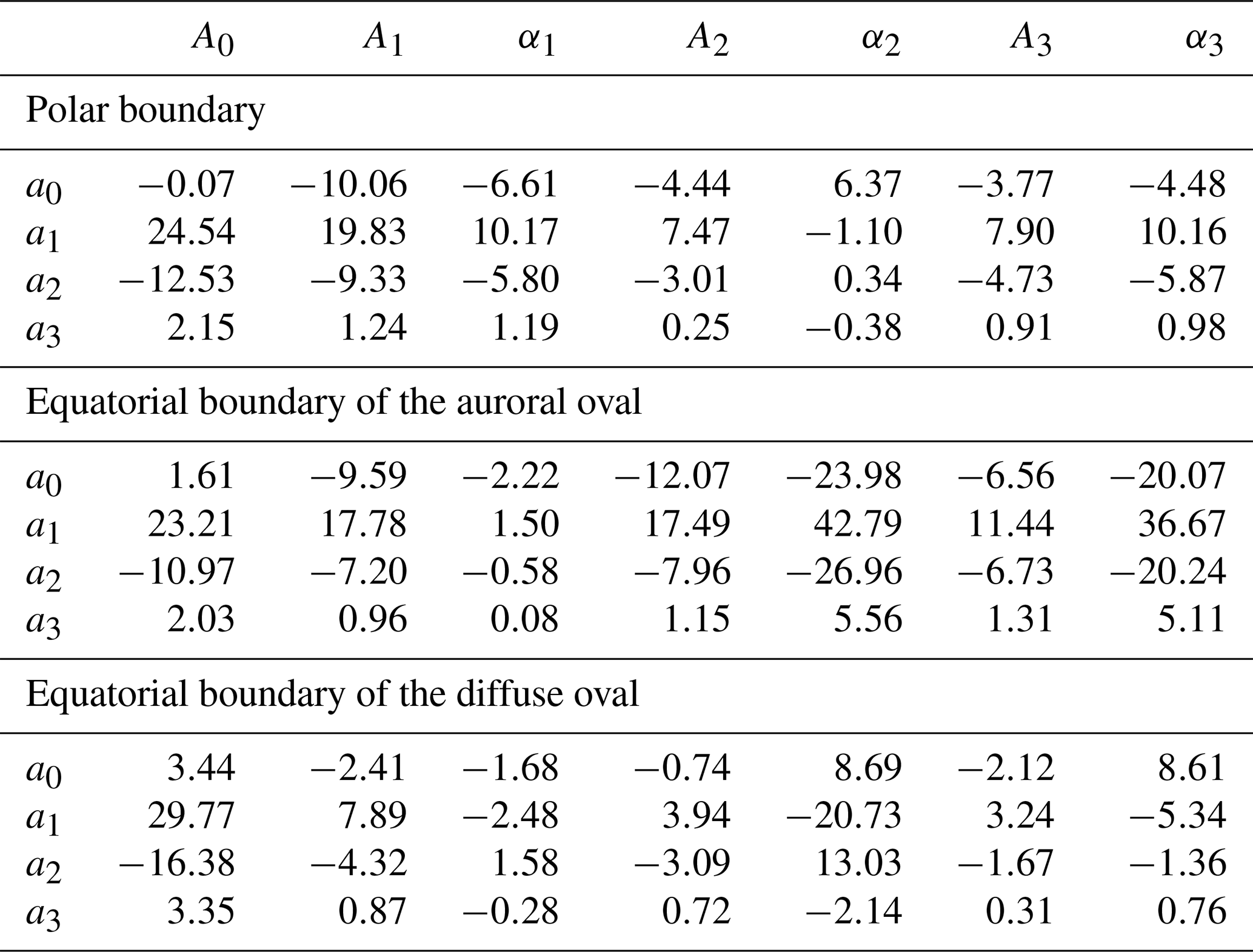
The Starkov (1994) model is actually an original Holzworth and Meng (1975) model of discrete and diffuse oval boundaries; however, it uses the AL index instead of the obsolete Q index as the input parameter. In our study, we only use discrete aurora boundaries.
where θ is boundary colatitude in corrected geomagnetic coordinates, Ai represents constants in degrees, t is the magnetic local time in hours, and αi represents constants in hours. The constants Ai and αi are determined separately for each boundary with respect to the AL index:
Regression coefficients are shown in Table A1.
Kamide et al. (1982) suggested the following estimate of the ionospheric east–west current density:
It is valid for the infinite equivalent ionospheric current approximation, assuming that the contribution from the ionospheric current to the observed magnetic perturbation is twice that of the induction current flowing in the Earth (similar to Eq. 4).
The IMAGE network data used in this paper can be downloaded from https://space.fmi.fi/image/www/index.php?page=request (last access: 15 January 2020), and the Yamal stations' data can be downloaded from http://serv.izmiran.ru/webff/magdb_all (last access: 28 December 2019).
MAE performed the data processing, and AAP was responsible for the data analysis and interpretation.
The authors declare that they have no conflict of interest.
The data analysis was funded by the Russian Science Fund (grant no. 18-47-05001). We are grateful to the IMAGE data archive and Aleksandr N. Zaitsev for the Yamal data.
This research has been supported by the Russian Science Foundation (grant no. 18-47-05001).
This paper was edited by Georgios Balasis and reviewed by Vladimir Papitashvili and one anonymous referee.
Akasofu, S.-I.: Polar and Magnetospheric Substorms, edited by: Reidel, D., Norwell, Mass, 18–19, 1968. a
Amm, O. and Viljanen, A.: Ionospheric disturbance magnetic field continuation from the ground to the ionosphere using spherical elementary current systems, Earth Planet. Space, 51, 431–440, 1999. a
Anderson, B. J., Takahashi, K., and Toth, B. A.: Sensing global Birkeland currents with Iridium® engineering magnetometer data, Geophys. Res. Lett., 27, 4045–4048, 2000. a
Chapman, S. and Bartels, J.: Geomagnetism, Oxford University Press, 1940. a
Feldstein, Ya. I. and Starkov, G. V.: Dynamics of auroral belt and polar geomagnetic disturbances, Planet. Space Sci., 15, 209–230, 1967. a
Ganushkina, N. Yu, Liemohn, M. W., and Dubyagin, S.: Current Systems in the Earth's Magnetosphere, Rev. Geophys., 56, 309–332, 2018. a
Gjerloev, J. W.: A global ground-based magnetometer initiative, Eos Trans. AGU, 90, 230–231, 2009. a
Holzworth, R. H. and Meng, C.-I.: Mathematical representation of the auroral oval, Geophys. Res. Lett., 2, 377–380, 1975. a
IMAGE: IMAGE network data, available at: https://space.fmi.fi/image/www/index.php?page=request, last access: 15 January 2020.
Johnsen M. G.: Real-time determination and monitoring of the auroral electrojet boundaries, J. Space Weather Space Clim.,3, A28, https://doi.org/10.1051/swsc/2013050, 2013. a
Kamide, Y., Akasofu, S.-I., Ahn, B.-H., Baumjohann, W., and Kisabeth, J. L.: Total current of the auroral electrojet estimated from the IMS Alaska meridian chain of magnetic observatories, Planet. Space Sci., 30, 621–625, 1982. a, b, c, d, e, f, g
Kotikov, A. L., Latov, Yu. O., and Troshichev, O. A.: Structure of auroral electrojets by the data from a meridional chain of magnetic stations, Geophysica, 23, 143–154, 1987. a, b, c
Mishin, V. M.: The magnetogram inversion technique and some applications, Space Sci. Rev., 3, 83–163, 1990. a
Papitashvili, V. O., Zaitsev, A. N., Rsatogi, R. G., and Sastri, N. S.: Proposed INDO-SOVIET collaborative studies based on the data along the Geomagnetic Meridian 145∘, Curr. Sci., 54, 666–671, 1985. a
Petrov, V. G.: Modeling of induction in the conducting earth in the study of the dynamics of polar electrojets, Geomagn. Aeron., 22, 159–161, 1982 (in Russian). a
Petrukovich, A. A., Mukai, T., Kokubun, S., Romanov, S. A., Saito, Y., Yamamoto, T., and Zelenyi, L. M.: Substorm-associated pressure variations in the magnetotail plasma sheet and lobe, J. Geophys. Res., 104, 4501–4513, 1999. a
Popov, V. A., Papitashvili, V. O., and Watermann, J. F.: Modeling of equivalent ionospheric currents from meridian magnetometer chain data, Earth Planet. Space, 53, 129–137, 2001. a, b, c
Pudovkin, M. I.: Sources of bay-like disturbances, Izv. Acad. Sci., 3, 484–489, 1960 (in Russian). a
Raeder, J., McPherron, R. L., Frank, L. A., Kokubun, S., Mukai, G. Lu, T., Paterson, W. R., Sigwarth, J. B., Singer, H. J., and J. A. Slavin: Global simulation of the Geospace Environment Modeling substorm challenge event, J. Geophys. Res., 106, 381–395, 2001. a
Slinker, S. P., Fedder, J. A., Ruohoniemi, J. M., and Lyon, J. G.: Global MHD simulation of the magnetosphere for November 24, 1996, J. Geophys. Res., 106, 361–380, 2001. a
Starkov, G. V.: Mathematical model of the auroral boundaries, Geomagn. Aeron., 34, 80–86, 1994 (in Russian). a, b, c, d, e, f
Untiedt, J. and Baumjohann, W.: Studies of polar current systems using the IMS Scandinavian magnetometer array, Space Sci. Rev., 63, 245–390, 1993 a
Viljanen, A. and Hakkinen, L.: IMAGE magnetometer network in Satellite-Ground Based Coordination Sourcebook, edited by: Lockwood, M., Wild, M. N., and Opgenoorth, H. J., Eur. Space Agency Spec. Publ., ESA SP-1198, 111–117, 1997. a
Vorobjev V. G., Yagodkina, O. I., and Katkalov, Y.: Auroral Precipitation Model and its applications to ionospheric and magnetospheric studies, J. Atmos. Terr. Phys., 102, 157–171, 2013. a
- Abstract
- Introduction
- Solution algorithms
- Model tests and algorithm adjustments
- Final algorithm for Model 3 with a small number of stations
- Discussion
- Conclusions
- Appendix A: Auroral oval boundaries
- Appendix B: Electrojet current density estimate
- Data availability
- Author contributions
- Competing interests
- Acknowledgements
- Financial support
- Review statement
- References