the Creative Commons Attribution 4.0 License.
the Creative Commons Attribution 4.0 License.
 | 05 Oct 2020
Ionospheric anomalies associated with the Mw 7.3 Iran–Iraq border earthquake and a moderate magnetic storm
Erman Şentürk
Samed Inyurt
İbrahim Sertçelik
The analysis of the unexpected ionospheric phases before large earthquakes is one of the cutting-edge issues in earthquake prediction studies. In this study, the total electron content (TEC) data from seven International GNSS Service (IGS) stations and the global ionosphere maps (GIMs) were used. Short-time Fourier transform (STFT) and a running median process were applied to the TEC time series to detect abnormalities before the Mw 7.3 Iran–Iraq border earthquake on 12 November 2017. The analyses showed positive anomalies 8–9 d before the earthquake and some positive and negative anomalies 1–6 d before the earthquake. These anomalies were cross-checked using the Kp, Dst, F10.7, Bz component of the interplanetary magnetic field (IMF Bz), electric field (Ey), and plasma speed (VSW) space weather indices. The results showed that the anomalies 1–6 d before the earthquake were caused by a moderate magnetic storm. Moreover, the positive anomalies 8–9 d before the earthquake were likely related to the Iran–Iraq border earthquake due to quiet space weather, local dispersion, and the proximity to the epicenter.
- Article
(6823 KB) - Full-text XML
- BibTeX
- EndNote


The ionosphere is a three-dimensional dispersive atmospheric layer for electromagnetic signals traveling from space to the Earth. The layer is located above a height of approximately 50–1000 km from the Earth's surface and includes molecules with the potential for photoionization. When molecules are exposed to light energy emitted from the Sun, their components are divided into atoms, which are negative electrons and positive ions. Negatively charged electrons affect the propagation of radio waves. To the first order, the degree of effect is a function of the number of free electrons. The Sun is the primary determiner of the number of electrons and causes permanent and regular ionospheric trends, such as daily, 27 d, seasonal, semiannual, annual, and 11-year trends (Vaishnav et al., 2019). The number of electrons also increases/decreases due to disturbed space weather (Bagiya et al., 2009), earthquakes (Liu et al., 2004; Şentürk et al., 2019), tsunamis (Occhipinti et al., 2013), volcanic eruptions (Dautermann et al., 2009), hurricanes (Chou et al., 2017), and anthropogenic events (Lin et al., 2017). These events generally cause non-secular changes, which are commonly referred to as ionospheric disturbances or ionospheric anomalies.
Global Navigation Satellite System (GNSS) technology provides low-cost, high-accuracy, near-real-time, continuous ionospheric data. GNSS-based TEC data have been preferred in many seismoionospheric studies related to large earthquakes (Liu et al., 2004, 2010; Fuying et al., 2011; Yildirim et al., 2016; Ulukavak and Yalcinkaya, 2017; Yan et al., 2017; Ke et al., 2018; Şentürk et al., 2019; Tariq et al., 2019). Liu et al. (2004) investigated 20 earthquakes with a magnitude greater than 6 in Taiwan between 1999 and 2002. They used GPS-based TEC data and applied the 15 d moving median and quartile range method to the TEC variation. The results showed that ionospheric abnormalities were detected before earthquakes with an 80 % success rate. Liu et al. (2010) reported seismoionospheric precursors to the 2004 Mw 9.1 Sumatra–Andaman earthquake due to anomalous decreases in the TEC variation 5 d before the earthquake. Fuying et al. (2011) used the Kalman filter method to detect abnormal changes in TEC variations before and after the Wenchuan Ms 8.0 earthquake. The TEC data were calculated from the GPS observations observed by the Crustal Movement Observation Network of China (CMONOC). The result showed that the Kalman filter is reasonable and reliable with respect to detecting TEC anomalies associated with large earthquakes. Yildirim et al. (2016) utilized 4 Continuously Operating Reference Stations in Turkey (CORS-TR) and 11 IGS and EUREF Permanent Network (EPN) stations to investigate the ionospheric disturbances related to the Mw 6.5 offshore earthquake in the Aegean Sea on 24 May 2014. TEC data from Precise Point Positioning (PPP-TEC), calculated using the PPP.PCF module in the Bernese software, and global ionosphere maps (GIMs) showed that the TEC values anomalously increased by 2–4 TECU (a TEC unit is equal to 1016 electrons m−2) 3 d before the earthquake and decreased by 4–5 TECU on the day before the earthquake. Ulukavak and Yalcinkaya (2017) used GNSS-based TEC data from six IGS stations to determine the pre-earthquake ionospheric anomalies before the Mw 7.2 Baja California earthquake on 4 April 2010. The results showed that both positive and negative ionospheric anomalies occurred 1–5 d before the earthquake. Yan et al. (2017) utilized data from CMONOC and IGS to statistically investigate the TEC anomalies before 30 Mw 6.0 + earthquakes from 2000 to 2010 in China. TEC anomalies were detected before 20 earthquakes, which equates to nearly 67 %. Ke et al. (2018) used a linear model between TEC and F10.7 to detect seismoionospheric TEC anomalies before and after the Nepal earthquake in 2015. The method was compared with sliding quartile and Kalman filter methods. They found that the linear model was more effective at detecting the TEC anomalies caused by the Nepal earthquake in temporal and spatial analyses. Şentürk et al. (2019) comprehensively analyzed the ionospheric anomalies before the Mw 7.1 Van earthquake on 23 October 2011, using temporal, spatial, and spectral methods. The results showed a 2–8 TECU increase in the TEC time series of 28 GNSS stations and GIMs before the Van earthquake on 9, 15–16, and 21–23 October. Tariq et al. (2019) used GNSS-based TEC data to detect the seismoionospheric anomalies of three major earthquakes (M>7.0) in Nepal and on the Iran–Iraq border from 2015 to 2017. The ionospheric precursors of the three earthquakes generally occurred within 10 d, between about 08:00 and 12:00 UT. The temporal and spatial statistical tests showed that the abnormal positive TEC changes were detected 9 d before the Mw 7.3 Iran–Iraq earthquake.
There is still no consensus on the physical process behind the changes in the ionosphere before earthquakes, but several assumptions have been made (Toutain and Baubron, 1998; Pulinets et al., 2006; Namgaladze et al., 2009; Freund et al., 2006, 2009; Freund, 2011). Toutain and Baubron (1998) reported that radon and other gases from the Earth's crust near the active fault progress toward the atmosphere and cause ionization. The increased radon release produces a unpronounced heat release (increasing air temperature) in the atmosphere by connecting the water molecules to the ions. This increase in air temperature leads to variability in air conductivity (Pulinets et al., 2006). The electron density in the ionosphere can increase or decrease due to this chaining process. Freund et al. (2006), in contrast, detected the ionization of the side surfaces of a granite block in the laboratory and proposed that the air was ionized due to an increase in the mechanical pressure applied to the upper surface. Under this assumption, strains occurring in the huge rocks in the lithosphere before earthquakes could cause electron emission towards the atmosphere and, therefore, may cause changes in the ionosphere (Freund et al., 2009).
In this study, temporal, spatial, and spectral analyses were applied to the GNSS-based TEC data to detect ionospheric anomalies before the Mw 7.3 Iran–Iraq border earthquake on 12 November 2017. Short-time Fourier transform (STFT) and a running median process were applied to define abnormalities in the TEC time series. The Kp, Dst, F10.7, Bz component of the interplanetary magnetic field (IMF Bz), electric field (Ey), and plasma speed (VSW) indices were also analyzed to show the effect of space weather on TEC variation. The paper is organized as follows: information on the Iran–Iraq border earthquake is given in Sect. 2.1; Sect. 2.2 presents data observations; Sect. 2.3 describes GPS-TEC and GIM-TEC data calculations; Sect. 2.4 capaciously explains the methods used in the study; and the results and conclusions are given in Sects. 3 and 4, respectively.
2.1 Iran–Iraq border earthquake
The deadliest earthquake of 2017 (with at least 630 casualties and more than 8100 people injured) occurred near the Iran–Iraq border (34.911∘ N, 45.959∘ E) at 18:18 UTC on 12 November 2017 and had a Mw 7.3 at a depth of 19.0 km (U.S. Geological Survey, 2017). The earthquake was felt in Iraq, Iran, and as far away as Israel, the Arabian Peninsula, and Turkey. The focal mechanism of the earthquake was identified as a thrust fault dipping at a shallow angle to the northeast (Wang et al., 2018). The earthquake occurred on the continental collision between Eurasian and Arabian plates, which is located within the Zagros fold and thrust belt.
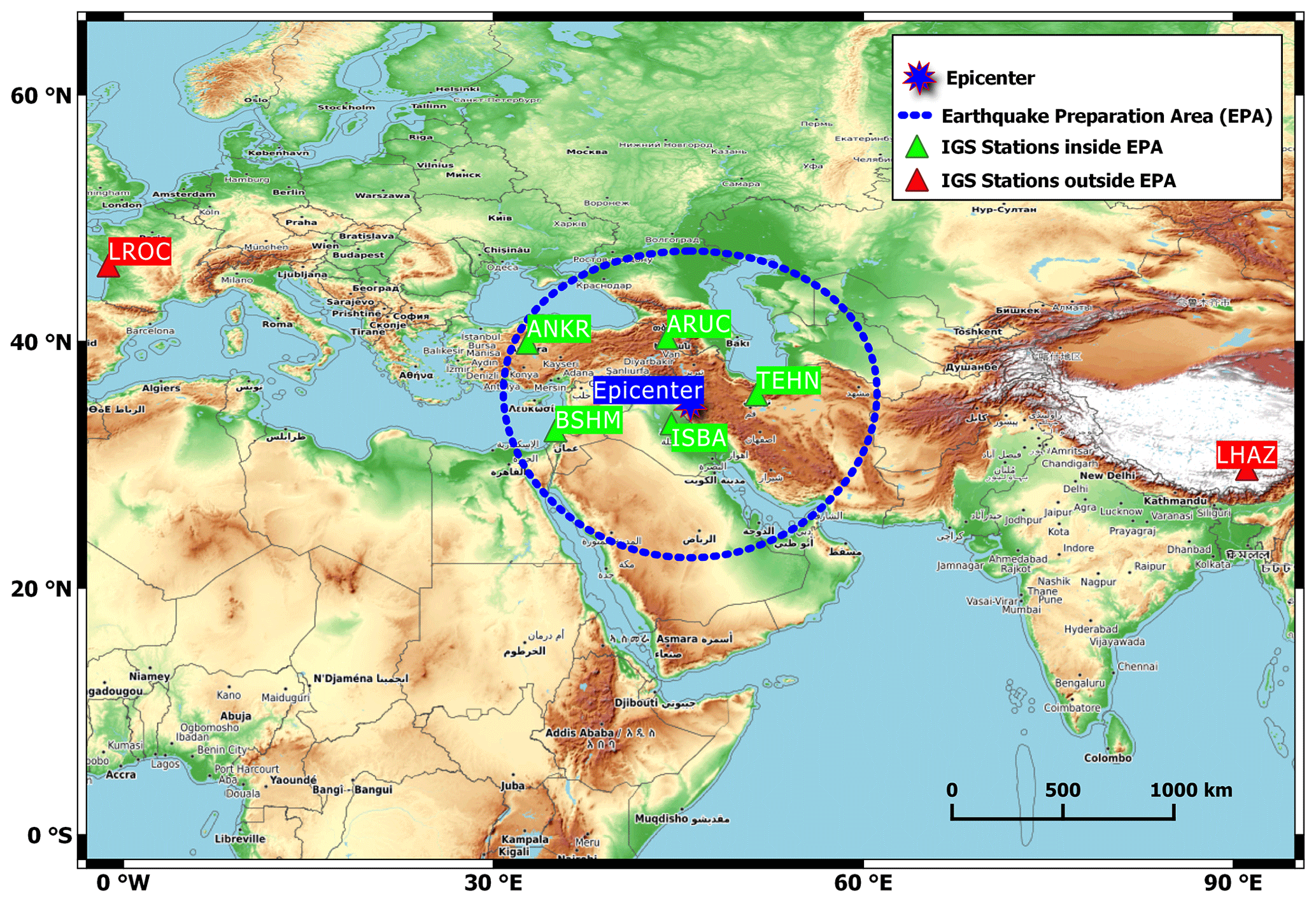
Figure 1The epicenter of the Iran–Iraq border earthquake, and the location of the IGS stations. The map of the area was sourced from https://opentopomap.org (last access: 28 June 2020).
2.2 The GNSS-based TEC data
The GNSS TEC data from seven IGS stations and GIMs produced by the Center for Orbit Determination in Europe (CODE) were used to investigate ionospheric anomalies before the Iran–Iraq border earthquake. The location of the IGS stations and the epicenter are shown in Fig. 1. The five IGS stations are selected within the earthquake preparation area (EPA), and the two IGS stations are located at a distance from the epicenter in order to reveal earthquake-induced anomalies. The Dobrovolsky equation was used to calculate the EPA as follows: r=100.43M km, where M is the magnitude (Dobrovolsky et al., 1979). The EPA was found to be 1380 km for the Iran–Iraq border earthquake. The distance of IGS stations from the epicenter and other information regarding the stations are given in Table 1. The geomagnetic coordinates of the stations were obtained from the KYOTO website (http://wdc.kugi.kyoto-u.ac.jp/igrf/gggm/, last access: 5 January 2020). Receiver Independent Exchange Format (RINEX) files for the IGS stations were downloaded from the IGS website (ftp://igs.ensg.ign.fr/pub/igs/data/, last access: 14 November 2019), and Ionosphere Map Exchange Format (IONEX) files from CODE were downloaded from the National Aeronautics and Space Administration (NASA) website (ftp://cddis.gsfc.nasa.gov/gps/products/ionex/, last access: 19 December 2019). The CODE GIMs cover ±87.5∘ latitudinal ranges and ±180∘ longitudinal ranges with a spatial resolution (5184 cells) and a 1 h temporal resolution (Dach et al., 2020).
The TEC describes the number of free electrons in a cylinder with a 1 m2 base area throughout the line of sight (LOS). The TEC unit (TECU) is equal to 1016 electron m−2. The linear integral of the electron density along the signal path ( corresponds to the slant total electron content (STEC). The STEC depends on the signal path geometry from the GNSS satellites (above a height of 20 000 km from the Earth's surface) to a receiver. The STEC is converted to the vertical total electron content (VTEC) using a mapping function. This conversion provides the number of free electrons along the LOS between the center of the Earth and a GNSS satellite. The VTEC is used for the input data for the global and regional ionosphere models, and it is a more useful parameter to define all ionization in the ionosphere. Assuming that all electrons are gathered in a thin layer, the TEC values at the receiver's zenith are obtained by the weighted average of the VTECs of all visible satellites (Schaer, 1999).
The effect of the ionosphere on the GNSS signal is directly proportional to the number of free electrons throughout the LOS and is inversely proportional to the square of the frequency of the GNSS signals (Hofmann-Wellenhof et al., 1992). The TEC parameter can be calculated with at least two different GNSS signal frequencies, because the effect of the ionosphere during the signal transition depends on the signal frequency. In recent years, some studies have also shown that the TEC can be calculated for single-frequency receivers using the Precise Point Positioning (PPP) technique, in which some parameters in the TEC calculation model are derived from IGS (Hein et al., 2016; Li et al., 2019).
In this study, the geometry-free linear combination () and “leveling carrier to code” algorithm is used to calculate the TEC values for seven IGS stations (Ciraolo et al., 2007). The L4 combination of carrier phase and code observations are as follows:
where α is a constant, f is the signal frequency, is the initial phase ambiguity (the i and k indices refer to the receiver and satellite, respectively), λ is the wavelength, is an integer, is the effect of the phase windup, c is the speed of light, bk is the satellite, and bi is the receiver differential code biases (DCBs). The DCBs of satellites and receivers are available in the daily IONEX files for IGS stations, but receiver DCBs for non-IGS stations must be calculated in the TEC calculation process. The phase-leveling technique is based on differences in the carrier phase and code observations on a continuous arc to reduce ambiguities from the carrier phase (L4).
In Eq. (3), the carrier phase observations are leveled with a bias produced by phase ambiguity. Finally, the STEC is calculated using Eq. (5):
The STEC is converted to VTEC using the single-layer model and a mapping function.
To define the number of free electrons in the receiver's zenith, the TEC is generally calculated by the weighted average of the VTECs of all visible satellites (Çepni and Şentürk, 2016).
Here, Wi indicates the weight of a satellite, which is generally described as a component of the satellite elevation angle , and n is equal to the number of visible satellites at any epoch.
The TEC values of the epicenter are interpolated from the nearest four grid points of GIMs using a simple four-point bivariate interpolation (Schaer et al., 1998).
where m and n are the latitudinal and longitudinal scale factors, respectively; βe and λe are the geocentric latitude and longitude of the epicenter, respectively; β0 and λ0 are the geocentric latitude and longitude of the nearest grid point, respectively; ΔβGIM and ΔλGIM are the spatial resolutions of the latitude and longitude of the GIMs, respectively; and VTEC00, VTEC01, VTEC10, and VTEC11 are the VTECs of the nearest grid points.
2.3 The short-time Fourier transform and running median methods
STFT is a method of obtaining the signal frequency information in the time domain as a modified version of the classical Fourier (Gabor, 1946). It provides an analysis of a small part of the signal at a particular time using the “windowing” technique (Burrus, 1995). This method divides the signal using a fixed time-frequency resolution (the size of the window is fixed in all frequencies) and presents the results in the time-frequency domain. It provides information about when and the frequencies at which a signal occurs. Thus, the method can provide statistical information about where and when the abnormality occurs in a TEC time series. The STFT of a signal is calculated as follows:
where f(t) is a time series (e.g., TEC), g(t) is the window function, τ is a shifting time variable, and ω is the angular frequency. Here, a discrete STFT that provided the identify and collected the frequency anomalies in the time domain was applied to obtain a time-frequency map of the TEC variation. A Gaussian window was also used as the window function g(t) (Harris, 1978):
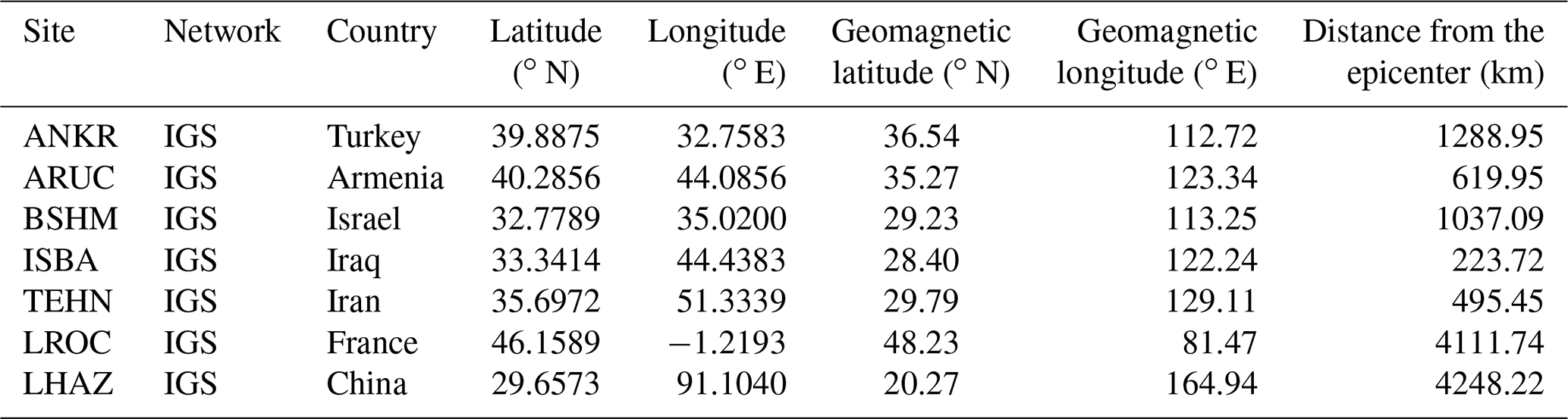
where N is the length of the window, and α could be termed as a frequency parameter. The width of the window is inversely related to the value of the width factor (α), and the α parameter controls the frequency resolution at both extremities. When the α value increases, the window becomes narrower; therefore, the selected α parameter gives relatively accurate resolution in the frequency domain (see Fig. 2). As it provided the best resolution, the α was chosen as 0.005 for this study.
A well-known anomaly detection method (running median) for seismoionospheric studies was used to validate STFT results. This method is based on the distribution moments median (M) and standard deviation (σ). In our analysis, the median of the TEC values for the previous 15 d was calculated in order to find the divergence from the observed TEC on the 16th day. The lower bound (LB) and upper bound (UB) were calculated using Eqs. (13) and (14), respectively, to assign the level of the divergence.
When the observed TEC for the 16th day exceeded the UB or LB, the positive or negative abnormal TEC signal was approved, respectively. An observed TEC between the UB and LB indicated no abnormal ionospheric condition. Assuming TECs are within a normal distribution with a mean μ and standard deviation σ, a 2σ divergence indicates that ionospheric phases are detected with a confidence level of about 95 %.
The degree of divergence of TEC values (DTEC; in percent) was also calculated using the deviation from median values in the GNSS TEC analysis. As DTEC provides the relative TEC, it is more successful in detecting abnormalities at dusk, when TEC values are lower.
3.1 Space weather before the earthquake
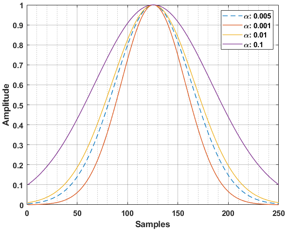
The Kp, Dst, F10.7, IMF Bz, Ey, and VSW space weather indices were cross-checked against the TEC times series to reveal the effects of space weather on TEC disturbances. The indices were obtained from the OMNI website (https://omniweb.gsfc.nasa.gov/form/dx1.html, last access: 2 February 2020). The time series of the indices for 15 d before the earthquake are given in Fig. 3.
Figure 3(a) IMF Bz and Ey, (b) VSW, (c) Dst, and (d) Kp and F10.7 indices for 15 d before the earthquake. The vertical black line indicates the earthquake event.
In Fig. 3a, the IMF Bz and Ey indices show some fluctuations on 1–2 and 7–11 November. These two indices remained calm on other days. From Fig. 3b, it can be noted that the VSW index increased rapidly from 300 to 650 km s−1 on 7 November. On the same day, the Dst index also decreased from +30 to −70 nT (see Fig. 3c). Both indices indicate a moderate magnetic storm (G2 level, Kp=6) on 7 November. On the other days, it was determined that the indices values were at levels where atmospheric conditions could be considered calm. In Fig. 3d, the F10.7 and Kp indices are shown. The F10.7 values remain quiet (<80 sfu) for the 15 d before the earthquake. The index ranges from 65 to 75 sfu. Kp values indicate disturbed magnetic conditions between 7 and 11 November, whereas other days have no magnetic activity values (Kp<4). Figure 3 suggests that the moderate magnetic storm that occurred 5 d before the earthquake was present until 1 d before the earthquake. The fluctuations in the IMF Bz and Ey indices on 1–2 November were not seen in other indices.
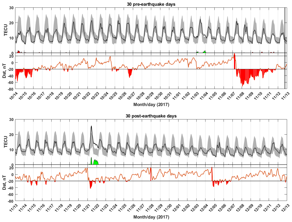
Figure 4TEC values of CODE GIMs over the epicenter, positive and negative anomalies, and Dst values during 30 pre- and post-earthquake days. The vertical black line indicates the earthquake event.
3.2 Temporal and spectral TEC variation of GNSS observations
TEC values over the epicenter location (34.911∘ N, 45.959∘ E) were obtained by interpolation from the VTEC values of the four grid points nearest to the epicenter in the GIMs in order to reveal ionospheric abnormalities in the zenith of the epicenter. The anomalies were detected using the running median method based on the median and ±2 standard deviations. In Fig. 4, TEC values of CODE GIMs over the epicenter, positive and negative anomalies, and Dst values are shown from 14 October to 13 December 2017. Figure 4 shows that non-storm-related abnormalities (1–2 TECU for 60 d) were only observed on 3–4 November, based on a period of 30 d before and after the earthquake.
In Fig. 5, the GNSS-based TEC time series from seven IGS stations – ANKR, ARUC, BSHM, ISBA, TEHN, LROC, and LHAZ – are presented. To better understand the earthquake-induced anomalies, the LROC and LHAZ stations were chosen outside of the EPA – at a distance from the epicenter. In the TEC calculation process, the satellite and receiver DCBs were obtained using IONEX files from CODE. The height of the single layer was selected as 450 km, and an elevation cutoff angle of 30∘ was taken. The sampling rate of TECs was 30 s. The results show that positive anomalies were detected on 3–4 November 2017, with 1–2 TECU at five stations inside the EPA. No apparent anomaly was detected at the two stations outside of the EPA on these dates. Some positive and negative anomalies were also determined on 7–12 November at all stations. Specifically, a 7 TECU positive anomaly was observed at the LROC station on 7 November. This anomaly is likely related to the moderate magnetic storm on 7–8 November.
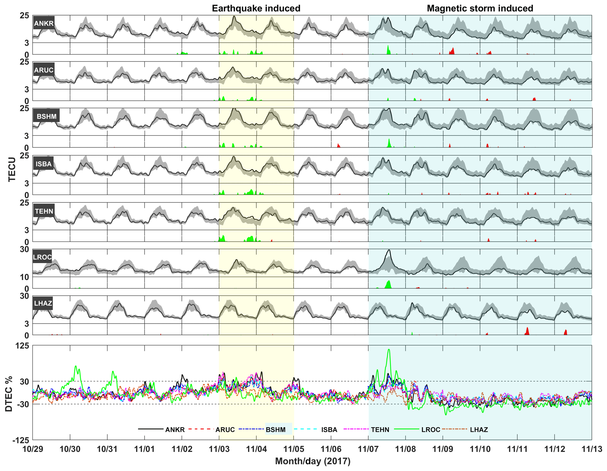
Figure 5The GNSS TEC variation for seven IGS stations. The solid black lines indicate the TEC values for the stations, and the gray areas demonstrate M±2σ. The positive and negative anomalies are shown using green and red areas, respectively. The transparent yellow area indicates earthquake-induced time intervals, and the transparent cyan area indicates magnetic-storm-induced time intervals. The bottommost graph shows the DTEC values for all IGS stations.
DTEC data from all of the IGS stations are given in the bottommost graph in Fig. 5. DTEC values reveal the relative change in the observed TEC values from the median TEC values. The ionosphere has significant day-to-day variability due to thermospheric dynamics even during quiet space weather (Forbes et al., 2000). Here, we selected the ±30 % limits for the day-to-day variability of the ionosphere. The ±30 % limits were exceeded in the positive direction on 2–5 and 7 November, and they were exceeded in the negative direction on 8–12 November. The highest positive DTEC value was detected on 4 November: +55 % at the ANKR station during the earthquake-induced time interval. During the storm-induced time interval, the highest positive DTEC was detected on 7 November (+115 %) and the lowest DTEC was detected on 9 November (−60 %) at the LROC station, which is located at the outside of the EPA. In Fig. 5, we show that the ±30 % limits for the DTEC variation are generally consistent with the quiet space weather condition of the running median method based on M±2σ.
In Fig. 6, the STFT method was applied as a spectral analysis of GNSS-based TEC data from five IGS stations inside the EPA with a 30 s sample rate. The method provides the TEC signals' predominant frequencies, where their “energies” reach the peak level of amplitudes related to frequencies and time. The amplitudes show the TEC values per hertz. At the ANKR station, high amplitude values are seen from 2 to 5 November and on 7 November; the highest amplitude value of about 30 TECU is seen on 3 November. At the ARUC station, high amplitudes are seen all day on 3 November. This station has a relatively smaller amplitude (∼24 TECU) value than the other stations. At the BSHM station, high amplitudes are seen on 3 and 7 November. At this station, the highest amplitude value of 29.5 TECU is seen on 7 November. At the ISBA and TEHN stations, high amplitudes are recognized on 3 November. The highest amplitudes are between 27 and 30 TECU. At all stations, the largest variations in the TEC anomalies correspond to smaller frequencies ( Hz), and the maximum amplitudes are between 25 and 30 TECU.
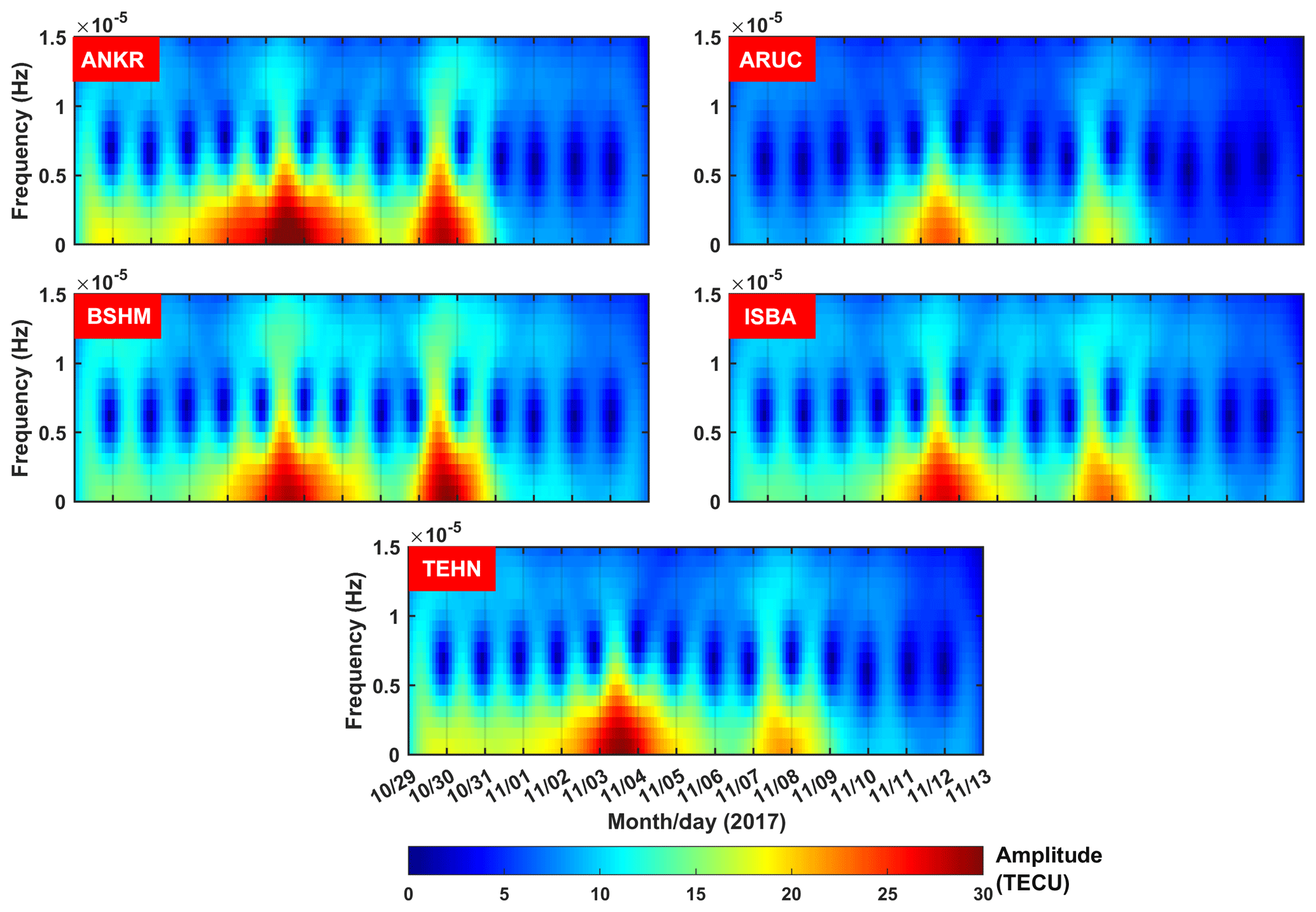
The STFT analysis had a high amplitude on the days of anomalies, which is defined in the running median method (see Fig. 5). Therefore, the STFT results are well correlated with classical methods. The fact that the STFT method reveals TEC anomalies without any background value is the strength of the method versus classical methods.
3.3 Spatial analysis of abnormal periods of TEC variation
The remarkably abnormal days (3, 4, 7, and 8 November) detected in the temporal and spectral analyses were spatially investigated using anomaly maps, which were created with CODE GIM data. These anomaly maps are bounded by 60∘ N–60∘ S latitudes and 180∘ W–80∘ E longitudes, and they have a temporal resolution of 2 h. In the maps, the epicenter of the earthquake is shown using a purple star. The TEC anomalies in the anomaly maps were detected using the running median method based on M±2σ. In Fig. 7, the anomalies have a range of ±5 TECU on 3–4 November. Figure 7 shows that the anomaly areas were locally distributed, and a notable anomaly area was concentrated near the earthquake epicenter. This area was located toward the northeastern side of the epicenter with 1–2 TECU from 14:00 to 02:00 UTC on 3–4 November. An anomaly area was also located on the southeastern side of the epicenter with 5 TECU from 04:00 to 06:00 UTC on 4 November. These anomalies are interesting because no other anomaly region is seen over a large area, and they are only located in close proximity to the epicenter. In Fig. 8, the anomalies have a range of ±10 TECU on 7–8 November. The only remarkable detail here is that the anomalies are distributed globally, as opposed to locally (as seen in Fig. 7). The changes detected on the relevant days mostly point to ionospheric variation caused by a magnetic storm.
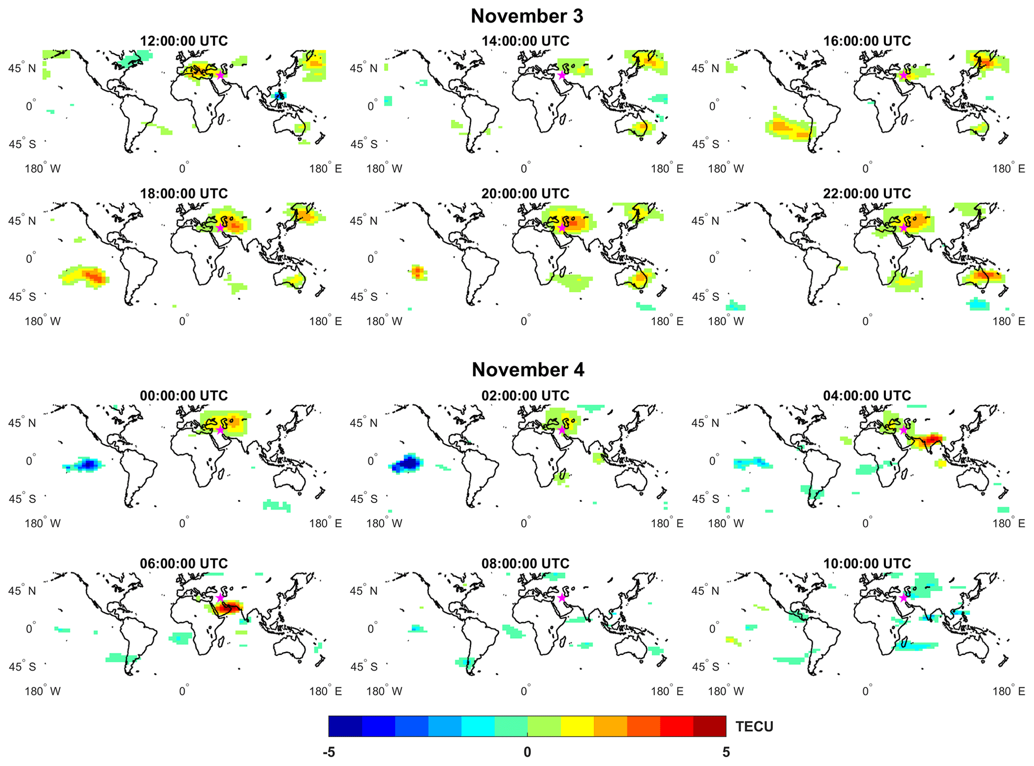
Figure 7The anomaly maps for 3–4 November 2017.
It is reasonable to argue that anomalies that occur at nighttime during calm space weather may be related to the earthquake or other phenomena, because the solar penetration towards the ionosphere decreases at night. Therefore, the anomalies detected between 18:00 UTC (21:00 LT) and 02:00 UTC (05:00 LT) on 3–4 November should be a precursor to the Iran–Iraq border earthquake due to the time of day (dusk), quiet space weather, and the local distribution.
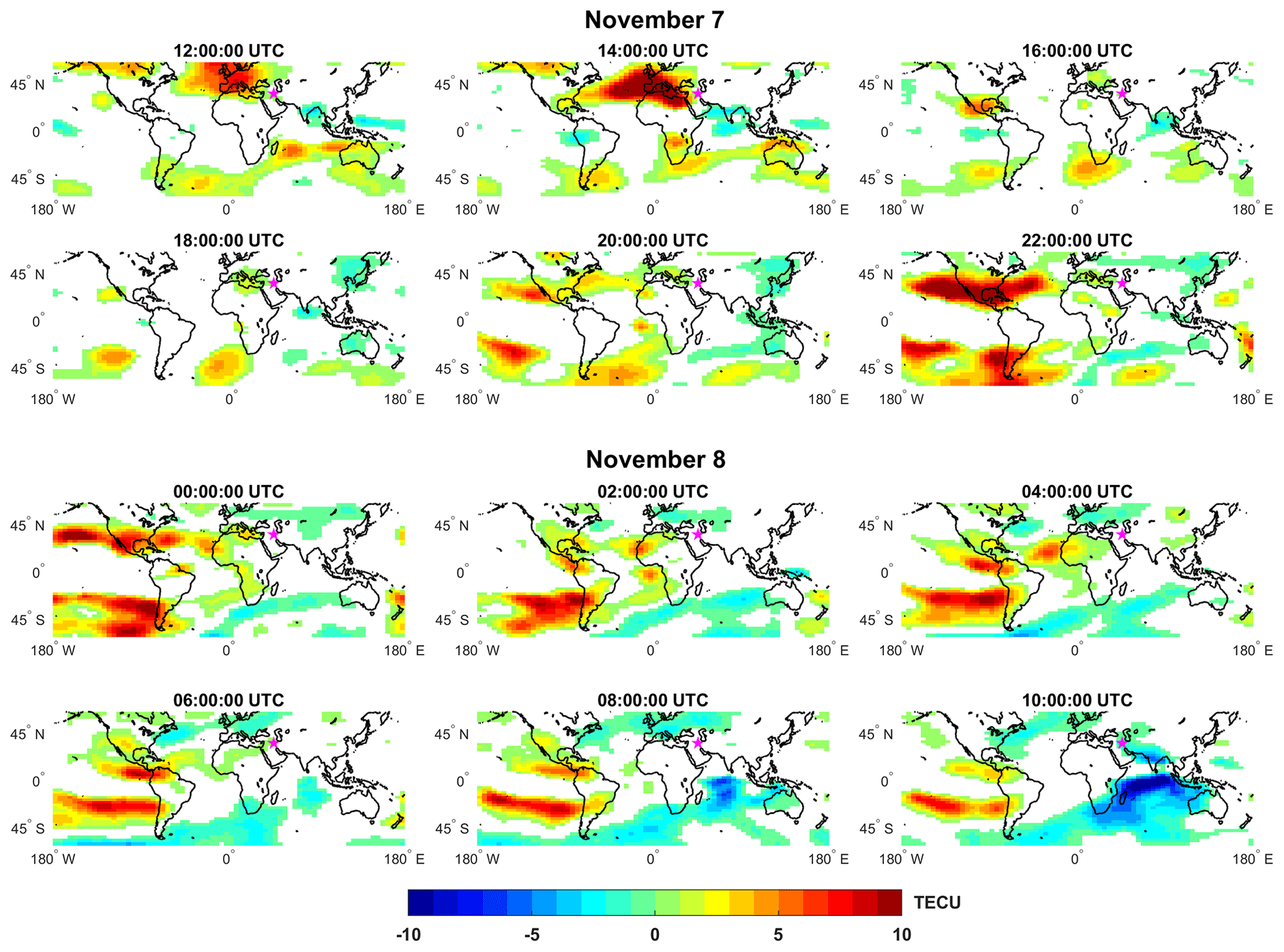
Figure 8The anomaly maps for 7–8 November 2017.
3.4 The prompt penetration electric field (PPEF) variation on abnormal days
PPEFs are the prompt reaction of the equatorial zonal electric field to solar wind alteration, which is a component of the interplanetary electric field (IEF) and the equatorial zonal electric field (Manoj et al., 2008). The penetration part of PPEFs (green line in Fig. 9) is calculated using interplanetary data, which are provided on the OMNI website. The quiet (climatological) part of PPEFs (violet line in Fig. 9), in contrast, is related to the 81 d moving average of the F10.7 solar flux (Manoj and Maus, 2012). The quiet and penetration parts of PPEFs were obtained from http://www.geomag.us/models/PPEFM/RealtimeEF.html (last access: 11 February 2020).
Figure 9 shows the prompt penetration electric fields (PPEFs) at 46∘ E longitude (geographical longitude of the epicenter) on 3–4 and 7–8 November. The PPEFs are observable in the ionosphere immediately after being transported to the magnetosphere by the solar wind (Tsurutani et al., 2008). The PPEFs also occur during periods with negative IMF Bz values (Astafyeva et al., 2016). Figure 3 indicates an increase in the solar wind from 300 to 650 km s−1 and a decrease in the IMF Bz to negative values of about −10 nT. Accordingly, fluctuations in PPEF variation are observed between 06:00 and 02:00 UTC on 7–8 November (see Fig. 9b). Many studies have reported that PPEFs cause positive and negative phases in the ionosphere during magnetic storms (Basu et al., 2007; Tsurutani et al., 2008; Mannucci et al., 2009; Lu et al., 2012; Astafyeva et al., 2016). Figure 9b indicates that the moderate magnetic storm caused the positive and negative anomalies in the ionosphere along with the change in PPEF values on 7–8 November. On the contrary, no significant difference in PPEF values was observed in Fig. 9a. These PPEFs values indicate that a magnetic storm or solar wind could not have affected the TEC variation on 3–4 November.
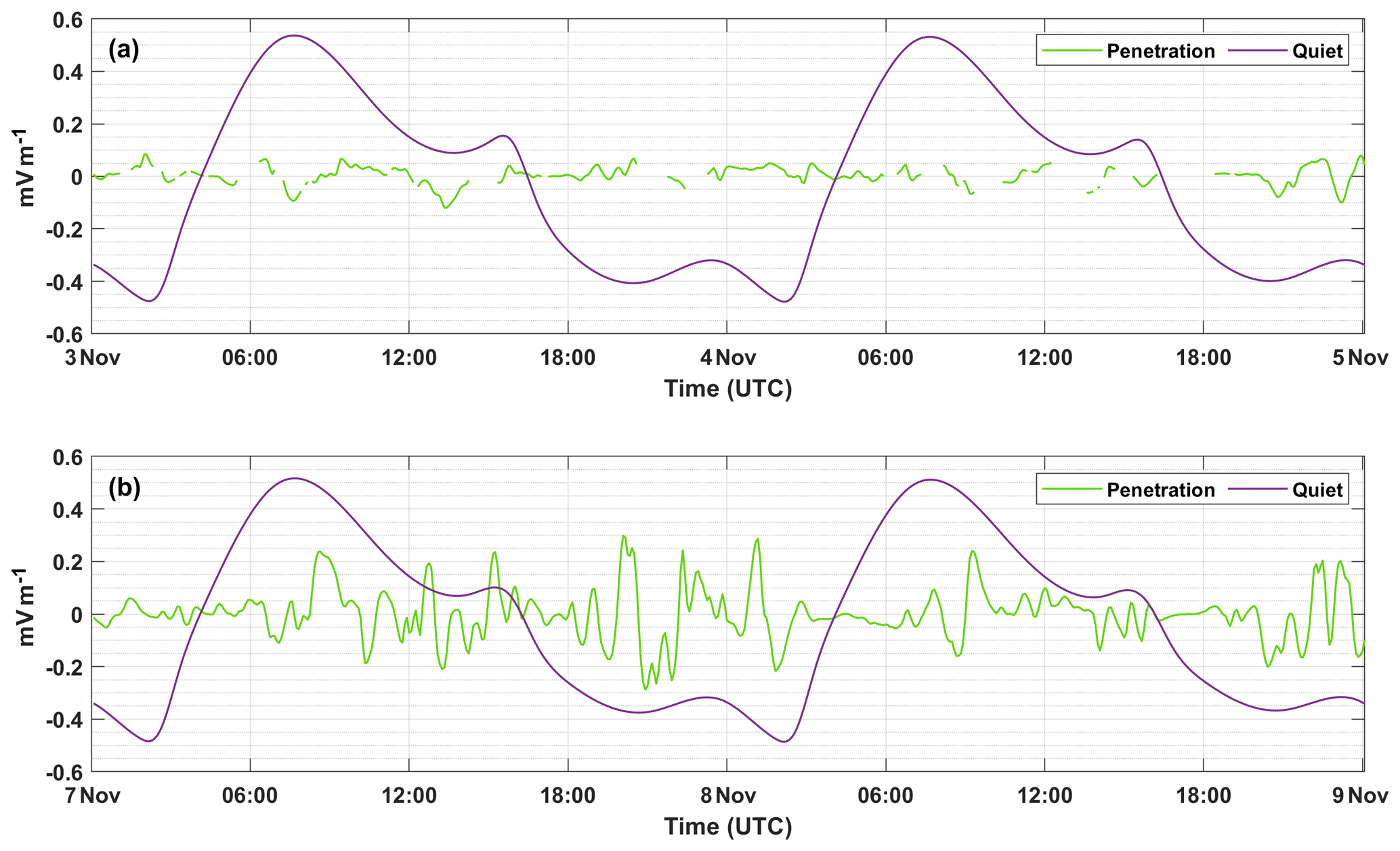
Figure 9The prompt penetration electric fields at 46∘ E longitude (a) on 3–4 November and (b) on 7–8 November 2017.
The TEC data from CODE GIM and seven IGS stations were analyzed to reveal the earthquake-induced ionospheric anomalies of the Mw 7.3 Iran–Iraq border earthquake. For this purpose, a classical method (the running median process) and the STFT method were applied to the TEC time series from 29 October to 13 November, 15 d before the earthquake. Only the CODE GIM time series were analyzed for 60 d, including 30 d before and after the earthquake. Thus, it was revealed that the anomalies obtained were not a coincidence. Abnormalities were only observed on 3–4 November, when the Dst values show quiet geomagnetic conditions ( nT). The running median process for TEC variation showed considerable positive anomalies of 1–2 TECU on 3–4 November in both the GIM and GNSS time series with the exception of the TEC time series of the LROC and LHAZ stations, which were located outside of the EPA. This value is calculated from the mean of a normal distribution with a width of 2 standard deviations, which is defined as a 95 % confidence level. These positive anomalies were also detected in the spectral analysis. The STFT method was used for spectral analysis. STFT is a powerful tool for processing a time series without any background values (mean, median, quiet days, and so on). The independence from background data minimizes the error sources of these data (unexpected changes and main trends of the ionosphere such as annual, semiannual, and seasonal variations). The results showed the power of the STFT method with respect to the detection of TEC anomalies..
There are some positive and negative anomalies 1–6 d before the earthquake, but these anomalies are likely caused by a moderate geomagnetic storm on 7–8 November. A geomagnetic storm affects the ionosphere as a whole, producing more global variations in TEC compared with the localized phenomena of seismoionospheric coupling. In Fig. 8, the global TEC changes in the moderate magnetic storm are seen. On the contrary, the anomalies occurring on 3–4 November, which are thought to have been caused by the earthquake, have a local distribution and are concentrated near the epicenter (see Fig. 7).
Although the space weather is rather quiet on 3–4 November, the DTEC values of the five IGS stations inside the EPA exceeded the ±30 % limits corresponding to the day-to-day variability of the ionospheric TEC and reached 55 %. This value indicates remarkable positive ionospheric anomalies. It can be said that the positive anomalies 8–9 d before the earthquake are likely associated with the Iraq–Iran border earthquake, as they occurred in close proximity to the epicenter and dispersed locally rather than globally. Moreover, the anomalies continued all day and were detected at all IGS stations inside the EPA.
This study presents the advantages of using different approaches to detect earthquake-related anomalies. Notably, spectral analysis methods are a new and promising approach that should be favored in future studies on the anomaly detection process.
The RINEX files of the IGS stations are publicly available at the IGS website: ftp://igs.ensg.ign.fr/pub/igs/data/ (last access: 14 November 2019, International GNSS Service, 2020). The IONEX files from CODE are publicly available at the NASA website: ftp://cddis.gsfc.nasa.gov/gps/products/ionex/ (last access: 19 December 2019, Center for Orbit Determination in Europe, 2020). The space weather indices are publicly available at the OMNI website: https://omniweb.gsfc.nasa.gov/form/dx1.html (last access: 2 February 2020, NASA/Goddard Space Flight Center, 2020).
ES carried out the data analysis, prepared the plots, and interpreted the results. SI provided processed GIM-based TEC time series. IS interpreted the storm-time effects on the ionosphere. ES prepared the paper with contributions from all authors.
The authors declare that they have no conflict of interest.
This paper was edited by Ana G. Elias and reviewed by two anonymous referees.
Astafyeva, E., Zakharenkova, I., and Alken, P.: Prompt penetration electric fields and the extreme topside ionospheric response to the June 22–23, 2015 geomagnetic storm as seen by the Swarm constellation, Earth Planets Space, 68, 152, https://doi.org/10.1186/s40623-016-0526-x, 2016.
Bagiya, M. S., Joshi, H. P., Iyer, K. N., Aggarwal, M., Ravindran, S., and Pathan, B. M.: TEC variations during low solar activity period (2005–2007) near the Equatorial Ionospheric Anomaly Crest region in India, Ann. Geophys., 27, 1047–1057, https://doi.org/10.5194/angeo-27-1047-2009, 2009.
Basu, S., Basu, Su., Rich, F. J., Groves, K. M., MacKenzie, E., Coker, C., Sahai, Y., Fagundes, P. R., and Becker-Guedes, F.: Response of the equatorial ionosphere at dusk to penetration electric fields during intense magnetic storms, J. Geophys. Res., 112, A08308, https://doi.org/10.1029/2006JA012192, 2007.
Burrus, C. S.: Multiband least squares FIR filter design, IEEE T. Signal Proces., 43, 412–421, 1995.
Center for Orbit Determination in Europe: IONEX files from CODE, ftp://cddis.gsfc.nasa.gov/gps/products/ionex/ (last access: 19 December 2019), 2020.
Çepni, M. S. and Şentürk, E.: Geometric quality term for station-based total electron content estimation, Ann. Geophys.-Italy, 59, A0107, https://doi.org/10.4401/ag-6803, 2016.
Chou, M. Y., Lin, C. C., Yue, J., Tsai, H. F., Sun, Y. Y., Liu, J. Y., and Chen, C. H.: Concentric traveling ionosphere disturbances triggered by Super Typhoon Meranti (2016), Geophys. Res. Lett., 44, 1219–1226, 2017.
Ciraolo, L., Azpilicueta, F., Brunini, C., Meza, A., and Radicella, S. M.: Calibration errors on experimental slant total electron content (TEC) determined with GPS, J. Geodesy, 81, 111–120, 2007.
Dach, R., Schaer, S., Arnold, D., Kalarus, M. S., Prange, L., Stebler, P., Villiger, A., and Jäggi, A.: CODE final product series for the IGS, Astronomical Institute, University of Bern, Bern Open Repository and Information System (BORIS), https://doi.org/10.7892/boris.75876.4, 2020.
Dautermann, T., Calais, E., Lognonné, P., and Mattioli, G. S.: Lithosphere-atmosphere-ionosphere coupling after the 2003 explosive eruption of the Soufriere Hills Volcano, Montserrat, Geophys. J. Int., 179, 1537–1546, 2009.
Dobrovolsky, I. P., Zubkov, S. I., and Miachkin, V. I.: Estimation of the size of earthquake preparation zones, Pure Appl. Geophys., 117, 1025–1044, 1979.
Forbes, J. M., Palo, S. E., and Zhang, X.: Variability of the ionosphere, J. Atmos. Sol.-Terr. Phy., 62, 685–693, 2000.
Freund, F. T.: Pre-Earthquake Signals: Underlying Physical Processes, J. Asian Earth Sci., 41, 383–400, 2011.
Freund, F. T., Takeuchi, A., and Lau, B. W.: Electric Currents Streaming Out of Stressed Igneous Rocks–A Step Towards Understanding Pre-Earthquake Low Frequency EM Emissions, Phys. Chem. Earth, 31, 389–396, 2006.
Freund, F. T., Kulahci, I. G., Cyr, G., Ling, J., Winnick, M., Tregloan-Reed, J., and Freund, M. M.; Air Ionization at Rock Surfaces and Pre-earthquake Signals. J. Atmos. Sol.-Terr. Phy., 71, 1824–1834, 2009.
Fuying, Z., Yun, W., and Ningbo, F.: Application of Kalman filter in detecting pre-earthquake ionospheric TEC anomaly, Geodesy and Geodynamics, 2, 43–47, 2011.
Gabor, D.: Theory of communication. Part 1: The analysis of information, Journal of the Institution of Electrical Engineers – Part III: Radio and Communication Engineering, 93, 429–441, 1946.
Harris, F. J.: On the use of windows for harmonic analysis with the discrete Fourier transform, IEEE, 66, 51–83, 1978.
Hein, W. Z., Goto, Y., and Kasahara, Y.: Estimation method of ionospheric TEC distribution using single frequency measurements of GPS signals, International Journal of Advanced Computer Science and Applications, 7, 1–6, 2016.
Hofmann-Wellenhof, B., Lichtenegger, H., and Collins, J.: Global Positioning System Theory and Practice, Springer-Verlag Wien, New York, 1992.
International GNSS Service: RINEX files of the IGS stations, website: ftp://igs.ensg.ign.fr/pub/igs/data/ (last access: 14 November 2019), 2020.
Ke, F., Wang, J., Tu, M., Wang, X., Wang, X., Zhao, X., and Deng, J.: Enhancing reliability of seismo-ionospheric anomaly detection with the linear correlation between total electron content and the solar activity index F10.7: Nepal earthquake 2015, J. Geodyn., 121, 88–95, 2018.
Li, M., Zhang, B., Yuan, Y., and Zhao, C.: Single-frequency precise point positioning (PPP) for retrieving ionospheric TEC from BDS B1 data, GPS Solutions, 23, 18, https://doi.org/10.1007/s10291-018-0810-2, 2019.
Lin, C. C., Shen, M. H., Chou, M. Y., Chen, C. H., Yue, J., Chen, P. C., and Matsumura, M.: Concentric traveling ionospheric disturbances triggered by the launch of a SpaceX Falcon 9 rocket, Geophys. Res. Lett., 44, 7578–7586, 2017.
Liu, J. Y., Chuo, Y. J., Shan, S. J., Tsai, Y. B., Chen, Y. I., Pulinets, S. A., and Yu, S. B.: Pre-earthquake ionospheric anomalies registered by continuous GPS TEC measurements, Ann. Geophys., 22, 1585–1593, https://doi.org/10.5194/angeo-22-1585-2004, 2004.
Liu, J. Y., Chen, Y. I., Chen, C. H., and Hattori, K.: Temporal and spatial precursors in the ionospheric global positioning system (GPS) total electron content observed before the 26 December 2004 M9.3 Sumatra–Andaman Earthquake, J. Geophys. Res., 115, A09312, https://doi.org/10.1029/2010JA015313, 2010.
Lu, G., Goncharenko, L., Nicolls, M. J., Maute, A., Coster, A., and Paxton, L. J.: Ionospheric and thermospheric variations associated with prompt penetration electric fields, J. Geophys. Res., 117, A08312, https://doi.org/10.1029/2012JA017769, 2012.
Mannucci, A. J., Tsurutani, B. T., Kelley, M. C., Iijima, B. A., and Komjathy, A.: Local time dependence of the prompt ionospheric response for the 7, 9, and 10 November 2004 superstorms, J. Geophys. Res., 114, A10308, https://doi.org/10.1029/2009JA014043, 2009.
Manoj, C. and Maus, S.: A real-time forecast service for the ionospheric equatorial zonal electric field, Space Weather, 10, 1–9, 2012.
Manoj, C., Maus, S., Lühr, H., and Alken, P.: Penetration characteristics of the interplanetary electric field to the daytime equatorial ionosphere, J. Geophys. Res., 113, A12310, https://doi.org/10.1029/2008JA013381, 2008.
Namgaladze, A., Klimenko, M. V. V., Klimenko, V., and Zakharenkova, I. E.: Physical Mechanism and Mathematical Modeling of Earthquake Ionospheric Precursors Registered in Total Electron Content, Geomagn. Aeronomy, 49, 252–262, 2009.
NASA/Goddard Space Flight Center: Interface to produce plots, listings or output files from OMNI 2, available at: https://omniweb.gsfc.nasa.gov/form/dx1.html (last access: 2 February 2020.
Occhipinti, G., Rolland, L., Lognonné, P., and Watada, S.: From Sumatra 2004 to Tohoku-Oki 2011: The systematic GPS detection of the ionospheric signature induced by tsunamigenic earthquakes, J. Geophys. Res.-Space, 118, 3626–3636, 2013.
Pulinets, S. A., Ouzounov, D., Karelin, A. V., Boyarchuk, K. A., and Pokhmelnykh, L. A.: The Physical Nature of Thermal Anomalies Observed before Strong Earthquakes, Phys. Chem. Earth, 31, 143–153, 2006.
Schaer, S.: Mapping and Predicting the Earth's Ionosphere Using the Global Positioning System, PhD thesis, University of Bern, Bern, Switzerland, 1999.
Schaer, S., Gurtner, W., and Feltens, J.: IONEX: The ionosphere map exchange format version 1, in: roceedings of the 1998 IGS Analysis Centers Workshop, ESOC, Darmstadt, Germany, 9–11 February 1998, 233–247, 1998.
Şentürk, E., Livaoğlu, H., and Çepni, M. S.: A Comprehensive Analysis of Ionospheric Anomalies before the Mw7.1 Van Earthquake on 23 October 2011, J. Navigation, 72, 702–720, 2019.
Tariq, M. A., Shah, M., Hernández-Pajares, M., and Iqbal, T.: Pre-earthquake ionospheric anomalies before three major earthquakes by GPS-TEC and GIM-TEC data during 2015–2017, Adv. Space Res., 63, 2088–2099, 2019.
Toutain, J. P. and Baubron, J. C.: Gas Geochemistry and Seismotectonics: A Review, Tectonophysics, 304, 1–27, 1998.
Tsurutani, B. T., Verkhoglyadova, O. P., Mannucci, A. J., Saito, A., Araki, T., Yumoto, K., Tsuda, T., Abdu, M. A., Sobral, J. H. A., Gonzalez, W. D., McCreadie, H., Lakhina, G. S., and Vasyliūnas, V. M.: Prompt penetration electric fields (PPEFs) and their ionospheric effects during the great magnetic storm of 30–31 October 2003, J. Geophys. Res., 113, A05311, https://doi.org/10.1029/2007JA012879, 2008.
Ulukavak, M. and Yalcinkaya, M.: Precursor analysis of ionospheric GPS-TEC variations before the 2010 M7.2 Baja California earthquake, Geomat. Nat. Haz. Risk, 8, 295–308, 2017.
U.S. Geological Survey: Earthquake Lists, Maps, and Statistics, available at: https://www.usgs.gov/natural-hazards/earthquake-hazards/lists-maps-and-statistics (last access: 28 March 2019), 2017.
Vaishnav, R., Jacobi, C., and Berdermann, J.: Long-term trends in the ionospheric response to solar extreme-ultraviolet variations, Ann. Geophys., 37, 1141–1159, https://doi.org/10.5194/angeo-37-1141-2019, 2019.
Wang, W., He, J., Hao, J., and Yao, Z.: Preliminary result for the rupture process of Nov. 13, 2017, Mw7.3 earthquake at Iran-Iraq border, Earth Planet. Phys., 2, 82–83, 2018.
Yan, X., Yu, T., Shan, X., and Xia, C.: Ionospheric TEC disturbance study over seismically region in China, Adv. Space Res., 60, 2822–2835, 2017.
Yildirim, O., Inyurt, S., and Mekik, C.: Review of variations in Mw<7 earthquake motions on position and TEC (Mw=6.5 Aegean Sea earthquake sample), Nat. Hazards Earth Syst. Sci., 16, 543–557, https://doi.org/10.5194/nhess-16-543-2016, 2016.