the Creative Commons Attribution 4.0 License.
the Creative Commons Attribution 4.0 License.
 | 09 Oct 2019
Wavelet analysis of the magnetotail response to solar wind fluctuations during HILDCAA events
Adriane Marques de Souza Franco
Ezequiel Echer
Mauricio José Alves Bolzan
In this work a study of the effects of the high-intensity long-duration continuous AE activity (HILDCAAs) events in the magnetotail was conducted. The aim of this study was to search the main frequencies during HILDCAAs in the Bx component of the geomagnetic field in the magnetotail, as well as the main frequencies, at which the magnetotail responds to the solar wind during these events. In order to conduct this analysis the wavelet transform was employed during nine HILDCAA events that coincided with Cluster spacecraft mission crossing through the tail of the magnetosphere from 2003 to 2007. The most energetic periods for each event were identified. It was found that 76 % of them have periods ≤4 h. With the aim to search the periods that have the highest correlation between the IMF Bz (OMNI) component and the Cluster Bx geomagnetic field component, the cross wavelet analysis technique was also used in this study. The majority of correlation periods between the Bz (IMF) and Bx component of the geomagnetic field observed also were ≤4 h, with 62.9 % of the periods. Thus the magnetotail responds stronger to IMF fluctuations during HILDCCAS at 2–4 h scales, which are typical substorm periods. The results obtained in this work show that these scales are the ones on which the coupling of energy is stronger, as well as the modulation of the magnetotail by the solar wind during HILDCAA events.
- Article
(3184 KB) - Full-text XML
- BibTeX
- EndNote


Geomagnetic activity occurs when there are disturbances in the Earth's magnetosphere caused by an enhanced solar-wind–magnetosphere energy transfer. The most known types of geomagnetic activities are the geomagnetic storms (Gonzalez et al., 1994), magnetic substorms (Akasofu, 1964) and HILDCAA (high-intensity long-duration continuous AE activity) (Tsurutani and Gonzalez, 1987). HILDCAA event is a kind of auroral activity and its cause is associated with the southward interplanetary magnetic field (IMF) Bz component of Alfvén waves (Tsurutani and Gonzalez, 1987; Tsurutani et al., 2004). These events are defined by four criteria: (i) the AE index has to attain at least one peak value ≥1000 nT, (ii) the event must last for a minimum of 2 d, (iii) the AE index cannot drop below 200 nT for more than 2 h at a time, and (iv) the event cannot occur during the main phase of a geomagnetic storm (Dst < −50 nT).
In the first studies that were done about HILDCAAs (Tsurutani et al., 1990, 2004), the question of whether these events could be a kind of continuous substorm arose. Tsurutani et al. (2004) proved the opposite, since those authors found that some substorms occurred with little or no changes in the AE index, which is the major characteristic observed during HILDCAA events. Thus, HILDCAAs are not necessarily geomagnetic substorms, although they may contain substorms in some cases. Another characteristic of HILDCAAs that distinguishes them from substorms is the aurora formed by these events. During HILDCAA events the auroras are weak or moderate, distributed in the whole auroral zone and can last several days, while during substorms, auroras are confined in small regions and last only 15 min (Guarnieri, 2006).
HILDCAAs are events of low Dst intensity, when compared with geomagnetic storms. However, the integrated energy input from particle precipitation into the ionosphere during the whole duration of a HILDCAA event can be bigger than the energy of moderate geomagnetic storms recovery phase (Guarnieri, 2005). Recent studies (Hajra et al., 2014; Mendes et al., 2017) of the energy transfer from solar wind to the magnetosphere and ionosphere during HILDCAAs have shown that two mechanisms are responsible for the energy and matter transfer, namely the magnetic reconnection (Dungey, 1961) and viscous interaction (Axford and Hines, 1961). Hajra et al. (2014) have shown the main process of solar wind energy dissipation in the magnetosphere during HILDCAA is by Joule heating in the auroral region, which is responsible for 67 % of the input energy. It was seen that the coupling between solar wind and the magnetosphere during these events occurs mainly in periods ≤8 h (Souza et al., 2018). Similar periods were observed in most energetic periods in the AE index and Bz IMF component. Those are comparable to the periods observed in the interplanetary Alfvén waves present in high-speed streams (HSSs) from coronal holes (Smith et al., 1995; Souza et al., 2016).
The magnetotail has an important role in the energy transfer from solar wind to the inner magnetosphere, since the energy of this process is stored in the tail (Lopez, 1990). During geomagnetic substorms, the solar wind energy is stored in the magnetotail during the initial phase and then in the expansion phase it is suddenly released and deposited in the ionosphere (Akasofu, 1981, 2013). This storage of energy can be interpreted as asymmetric ring currents and magnetotail currents, which respond to the periods of substorms that were observed as 2–4 h (Sitnov et al., 2001). The aim of this work is to identify the main periodicities present in the geomagnetic field Bx component in the magnetotail during HILDCAA events, and also to study at which periods the energy is preferentially transferred from the solar wind to that region during these geomagnetic disturbances using wavelet analyses.
In order to develop this study, geomagnetic field Bx component data obtained by the fluxgate magnetometer (FGM) (Balogh et al., 2001) from the satellite SC4 of the Cluster constellation (https://csa.esac.esa.int/csa-web/#search, last access: 7 October 2019) with 4 s resolution were used. The Bx component corresponds to the Sun–Earth line direction, and it is an indicator of when the Cluster spacecraft crosses the magnetic equator in the tail and is also an indicator for the stretching or depolarization of the tail field (e.g. see Korth et al, 2006; Echer et al., 2017). Nine events were selected (one in August 2003, two in September 2003, one in October 2003, one in September 2004, one in August 2005, two in October 2006 and one in September 2007), which correspond to the events when Cluster crossed the plasma sheet during the occurrence of HILDCAAs. In this analysis AE and IMF Bz component data were also used. The AE indices at 1 min time resolution were obtained from the World Data Center for Geomagnetism, Kyoto, Japan (http://wdc.kugi.kyoto-u.ac.jp/, last access: 30 September 2019), and the IMF Bz data (1 min) were obtained from the OMNI web (http://omniweb.gsfc.nasa.gov/, last access: 30 September 2019). In this paper Cluster and IMF data are in the Geocentric Solar Ecliptic (GSE) coordinate system.
Table 1 shows some relevant information about the HILDCAA events that were analyzed, where the start and end times of each event are shown, as well as the data intervals analyzed for the Cluster magnetotail crossings.
Table 1Bx geomagnetic field component data information used for the HILDCAA events analysis in the magnetotail.
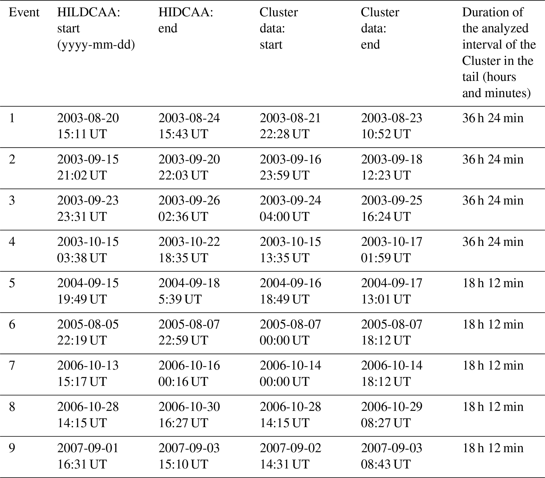
Figure 1 shows the time series during the HILDCAA event that occurred between 03:38 UT on 15 October to 18:35 UT on 22 October 2003 (event 4 in Table 1). Panel (a) shows the IMF Bz component, (b) the Cluster tail Bx component, and (c) the AE index. From this figure it is possible to observe HIDLCAA features in the IMF Bz and AE index data, where Alfvénic fluctuations can be observed in the IMF Bz data. In the AE time series, the values of the index can reach peaks higher than 1000 nT. The blue line in the AE index panel corresponds to the 200 nT value, where we can note that the AE index is lower than this value only for short intervals of time. The interval on which the Cluster crossed the magnetotail during the event is marked with the red rectangle on the panels.
The intervals of the Cluster crossing the magnetotail during HILDCAAs selected for our study were identified by analyzing the orbit of the spacecraft during the HILDCAA events, where these nine events were obtained. The Cluster orbit in the XZ plane for the HILDCAA plotted in Fig. 1 is shown in Fig. 2, where the Cluster magnetotail crossing is marked in pink on the orbit panel.
Non-stationary time series can be analyzed by wavelet transform (WT), a powerful mathematical tool that is able to show the temporal variability of the power spectral density (Morettin, 1992). Wavelet functions ψ(t) are generated by a simple function called wavelet mother, shown in Equation 1, which suffers expansion ψ(t)→ψ(2t) and translations in time, giving rise to those wavelet functions well known as wavelet daughters (Torrence and Compo, 1998).
where a represents the scale associated to the dilation and contraction of the wavelet, and b is the temporal location, which relates to the translation in time.
The WT applied on f(t) time series is defined as follows:
where f(x) is the time series, ψa,b(t) is the wavelet function and represents the complex conjugate thereof.
The wavelet function can be characterized by using two types of functions, the continuous and discrete ones (Daubechies, 1992). The discrete wavelets are used for decomposition of time series in frequency, which is useful for the filtering process. Among the most known functions are the Meyer, Daubechies and Haar functions (Grinsted et al., 2004). The continuous wavelet functions allow the separation of phase and amplitude components associated with the signal; therefore they are generally used for analysis of time series. The most common continuous wavelet functions are the Mexican hat and the Morlet functions (Torrence and Compo, 1998; Addison, 2018). In this paper, both a discrete and a complex wavelet function were used, the Haar function in order to remove long-term trends in the data and the Morlet function for the periodicity identification.
As Cluster spacecraft travels through large spatial and latitudinal ranges, where the Earth's magnetic field has strong dependence, the magnetic field sampled by Cluster data has large spatial variations. These are noted in time as a long-term trend, as can be observed in Fig. 1c, in the geomagnetic Bx component. These long-term effects observed in the geomagnetic field Bx component data can affect the results of the periodicities identified by wavelet analysis. In order to remove it, a technique of long-term trend extraction using the Haar wavelet function was applied in the data. The Haar wavelet function is the simplest type of wavelet and has been used since 1910 (Haar, 1910; Porwik and Lisowska, 2004). The Haar function is defined as a complete orthogonal system of functions which have a dyadic dilatation a=2j and with translations in discrete steps () (Porwik and Lisowska, 2004; Bolzan et al., 2009; work in progress). The Haar wavelet function is shown in Eq. (3):
where j and k are integers.
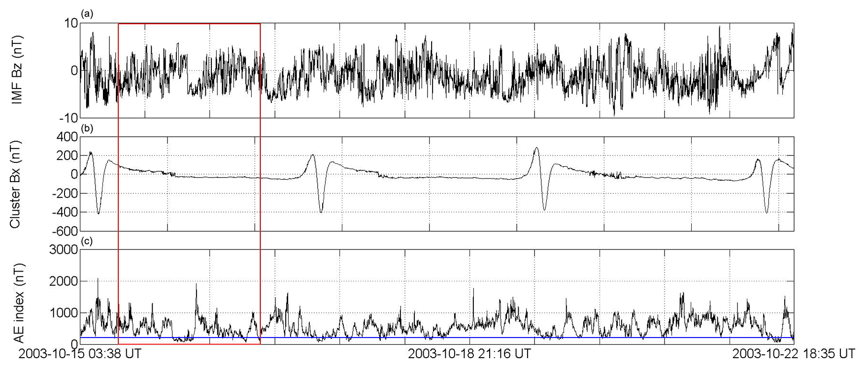
Figure 1Time series of IMF Bz (a), Cluster Bx (b) and AE index (c) for the HILDCAA event that occurred from 03:38 UT on 15 October to 18:35 UT on 22 October 2003.
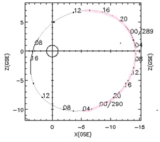
Figure 2Cluster orbit in the XZ plane for the HILDCAA that occurred from 03:38 UT on 15 October to 18:35 UT on 22 October 2003 (event number 4 in Table 1). The axes are plotted in Earth radii. The part of the orbit marked by pink represents the interval on which the Cluster crossed the magnetotail during the event.
The detrending method consists of applying a Haar wavelet transform function in the data, which decomposes them in dyadic scales, after identifying the scales where the long-term periodicities are present; these scales are removed from the data, in such a way that the main characteristics of the time series are maintained (Bolzan et al., 2019). Figure 3 shows an example where this technique was applied in the geomagnetic field Bx component in the magnetotail during a HILDCAA event that occurred from 22:19 UT on 5 August to 22:54 UT on 7 August 2005 (event 6, Table 1). Panel (a) shows the original time series where the long trend can be observed, and (b) shows the time series after filtering the scales and removing the long-term trend.
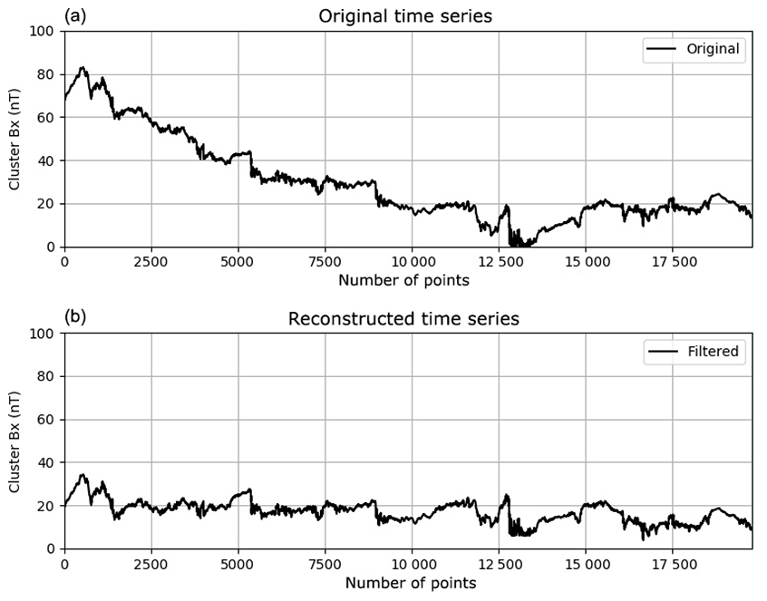
Figure 3Geomagnetic field Bx component data for the interval that the Cluster was in the magnetotail during the HILDCAA event, which occurred between 22:19 UT on 5 August to 22:54 UT on 7 August 2005. Panel (a) shows the original data and (b) shows the detrended data after removal of the long tendency. In (a) and (b) the x axes represents the number of points.
After detrending the long-term trend in the data, the Morlet wavelet was applied with the aim of identifying the main periodicities present. The Morlet wavelet is a plane wave modulated by a Gaussian envelope and can be described by Eq. (4) (Torrence and Compo, 1998):
where ξ0 represents the dimensionless frequency. In this work this value of parameter was set up as 6.0, since its shape gives good localization in time (Torrence and Compo, 1998).
The global wavelet spectrum (GWS) shows the integrated energy in time for each frequency. Consequently, the GWS is useful for the identification of the most energetic frequencies and periods in a time series. The GWS is given as follows:
This study also aims to identify the periods in which the energy transfer from the solar wind to the magnetotail and auroral zone is more efficient during HILDCAA events. In order to obtain that, the cross-wavelet transform (XWT) was used. The XWT (Eq. 6) is constructed from two continuous WT of two time series, which allows analysis of the correlation between the time series as a function of the signal period and its temporal evolution identifying their power in common (Grinsted et al., 2004; Bolzan et al., 2012).
where Wx and Wy represent the WT applied to the time series x(t) and y(t), and (*) represents the complex conjugate of the WT.
In order to study the main periods with higher correlation between two time series the global correlation spectrum (GCS) is computed. The GCS can be obtained by rewriting Eq. (5) as follows:
where σx and σy represent the variances of the time series x(t) and y(t), respectively.
After removing the long-term trend of the Cluster Bx data, the WT was applied on the detrended Bx series in order to identify the main periodicities in the geomagnetic Bx component in the magnetotail. The XWT was also computed for the identification of the periods with higher correlation between the Cluster Bx component and IMF Bz component and also between the Cluster Bx component and AE index.
4.1 Periodicities in the Bx geomagnetic component
Figure 4 shows the WT applied to the geomagnetic Bx component during the HILDCAA event that occurred from 22:19 UT on 5 August to 22:54 UT on 7 August 2005 (same interval of Fig. 3), for the period when the Cluster crossed the magnetotail, between 00:00 and 18:12 UT on 7 August 2005, Fig. 4a the Bx filtered time series, Fig. 4b the wavelet power spectrum and Fig. 4c shows the 2 most energetic periods present in the data marked, the first at 1.6 h and the second at 4.0 h.
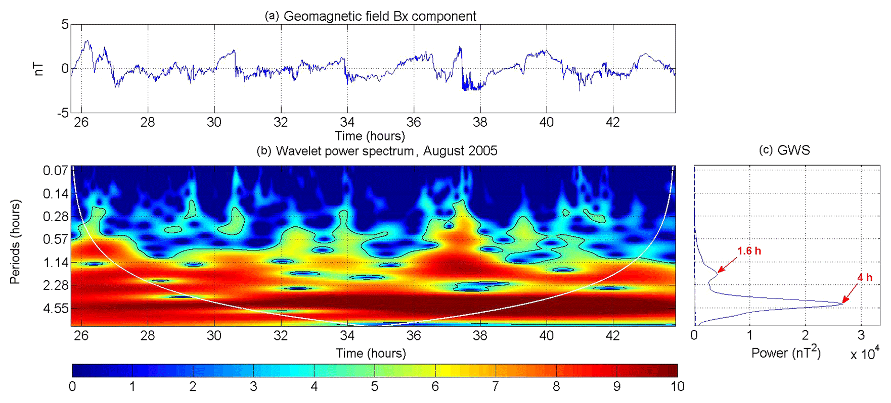
Figure 4(a) Filtered geomagnetic magnetotail field Bx component time series for the interval that the Cluster remained in the magnetotail during the HILDCCA event that occurred between 22:19 UT on 5 August and 22:54 UT on 7 August 2005. (b) Wavelet power spectrum. (c) GWS. In (a) and (b), the x axes represent the number of hours after the HILDCAA event started.
With the goal of identifying the main periods of the Bx geomagnetic component, the periods with peaks of energy found in the GWS (the most energetic periods) plots in all events were divided into bins of 2 h. A total of 25 periods between 0 and 8 h were identified and the result of this analysis is shown in the histogram of Fig. 5.

Figure 5Histogram of the percentage of the main frequencies in Bx geomagnetic field component in the magnetotail during HILDCAAs.
All periods here noted in the geomagnetic Bx component were found in the same range observed by Souza et al. (2016) for the most energetic periods found in the IMF Bz component, using 52 HILDCAAs that occurred between 1995 and 2011.
From Fig. 5 it is possible to note that the most energetic periods were shorter than or equal to 8 h. It was observed that 76 % of the 25 periods identified occurred in the interval ≤4 h. Although few events were used for this study, it is worth noting that the major energetic periodicities here found correspond to the periods obtained by Borovsky et al. (1993) in a study of the time interval between substorm onsets, where a major period of 2.75 h was identified. Those authors have interpreted this period as a loading–unloading substorm cycle. Lee at al. (2006) also observed that repetitive substorms caused by Alfvén waves in the IMF during HSS have periods of 1–4 h. Similar results were also found by Korth et al. (2006) in the study of events of HSS, wherein substorms were observed with periods between 2 and 4 h. Also, Bolzan et al. (2012) using ACE IMF and Cluster magnetic field data had found similar periods, 2.3 h, during storms driven by corotating interaction regions (CIRs).
The energy distribution in the main periods observed in the geomagnetic Bx component during HILDCAA was studied using the classification introduced by Souza et al. (2016). The energy distribution can be classified in four forms: local, intermittent, quasi-continuous and continuous. Local classification is characterized by the distribution of energy which occurred in only one intense region during the event. In the intermittent type distribution one can observe the presence of energy in small regions located in time, but scattered at various moments during the event. In the quasi-continuous distribution, the range of periods with intense energy can be observed in almost the whole event. And in the continuous type, a range of intense energy can be observed in the whole event. For this study we also count the number of the most energetic periods which fit in each classification, and then a table with the percentage of each behavior was generated and presented (Table 2).
The results shown in Table 2 indicate that most of the HILDCAA periods showed their energy distribution with the continuous form, present in 32 % of the 25 periods observed inside the cone of influence. Note that 52 % of the periods are quasi-continuous or intermittent, which means they are transient events, which is a characteristic of substorms (Hones Jr., 1979).
4.2 Correlation between IMF Bz and geomagnetic Bx components
The XWT was applied to the data of IMF Bz component (GSM) and the Bx geomagnetic component, in order to search for periods with high correlation between these two time series. Obtaining these periods is important to identify the frequencies on which the coupling of energy is stronger, as well the modulation of the magnetotail by the solar wind during HILDCAA events (Korth et al., 2006; Bolzan et al., 2012). The classification of the characteristic form of the periods with higher correlations obtained by the XWT was also done.
The XWT of the HILDCAA which occurred from 15:11 UT on 20 August to 15:43 UT on 24 August 2003 (first event in Table 1) is presented in Fig. 6. Figure 6a shows the time series of IMF Bz component and Bx geomagnetic component time series, (b) the XWT between those two time series, and (c) the global cross wavelet spectrum. In Fig. 6c it is possible to observe three periods with higher values of correlations, related to the periodicity types characterized as intermittent, local and quasi-continuous, respectively, in Fig. 6b. The first peak of correlation has a period of 1.2 h, the second of 3.2 h, and the last one of 5.7 h.
Table 2Energy distribution classification of the geomagnetic Bx component during HILDCAAs.

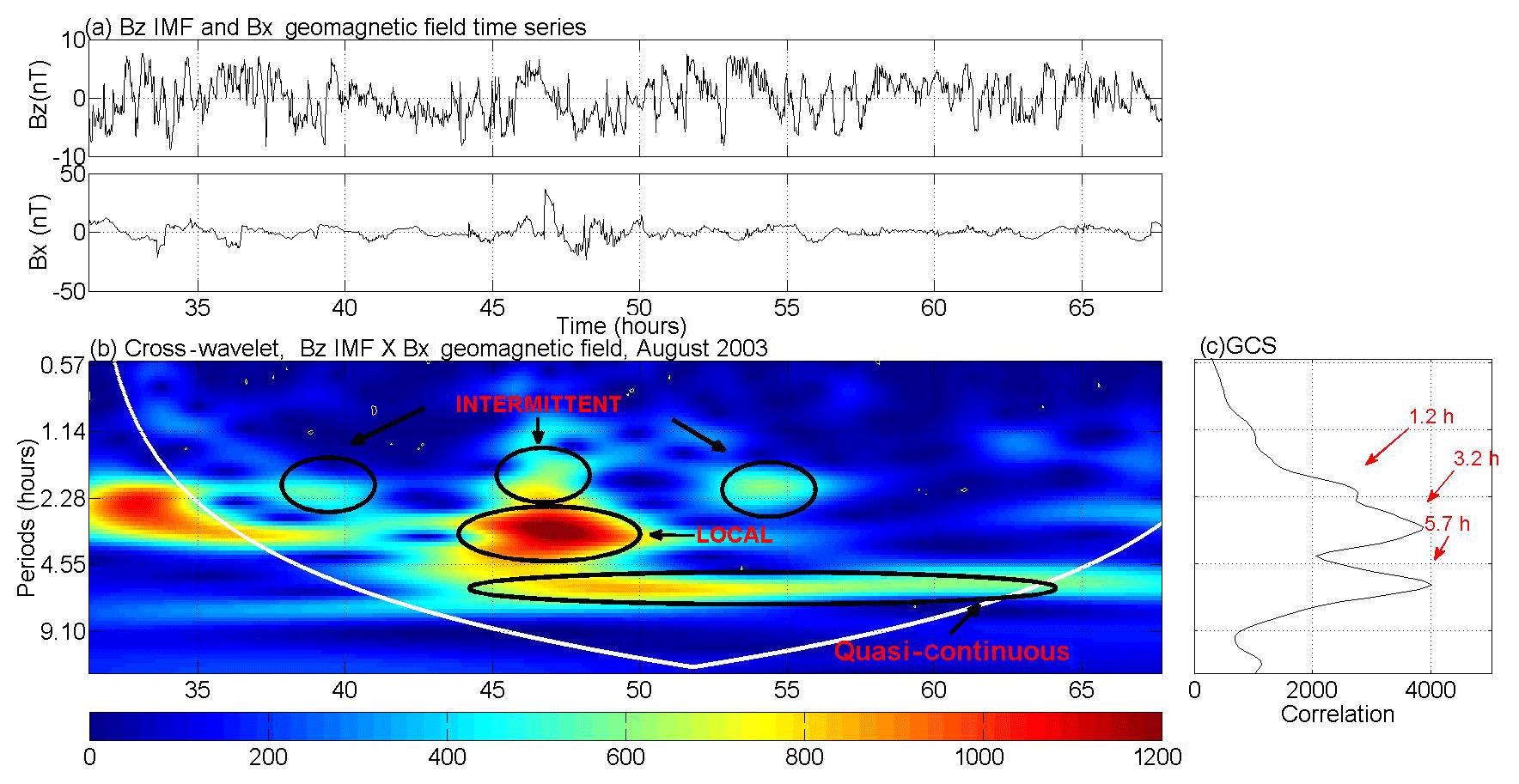
Figure 6(a) Bz IMF and filtered Bx geomagnetic field time series. (b) Cross wavelet spectrum. (c) Global correlation spectrum. In (a) and (b) the x axes represent the number of hours after the HILDCAA event started.
A total of 27 periods of high correlation was identified between Bz IMF (GSM) and the Bx geomagnetic component observed in these nine HILDCAA events. These periods were also divided into ranges of 2 h and the percentage of the number of periods identified in each interval is presented in the histogram of Fig. 7. Through Fig. 7, it possible to see that the energy transfer is more efficient for periods ≤4 h, which presented 62.9 % of the signals with higher correlation.
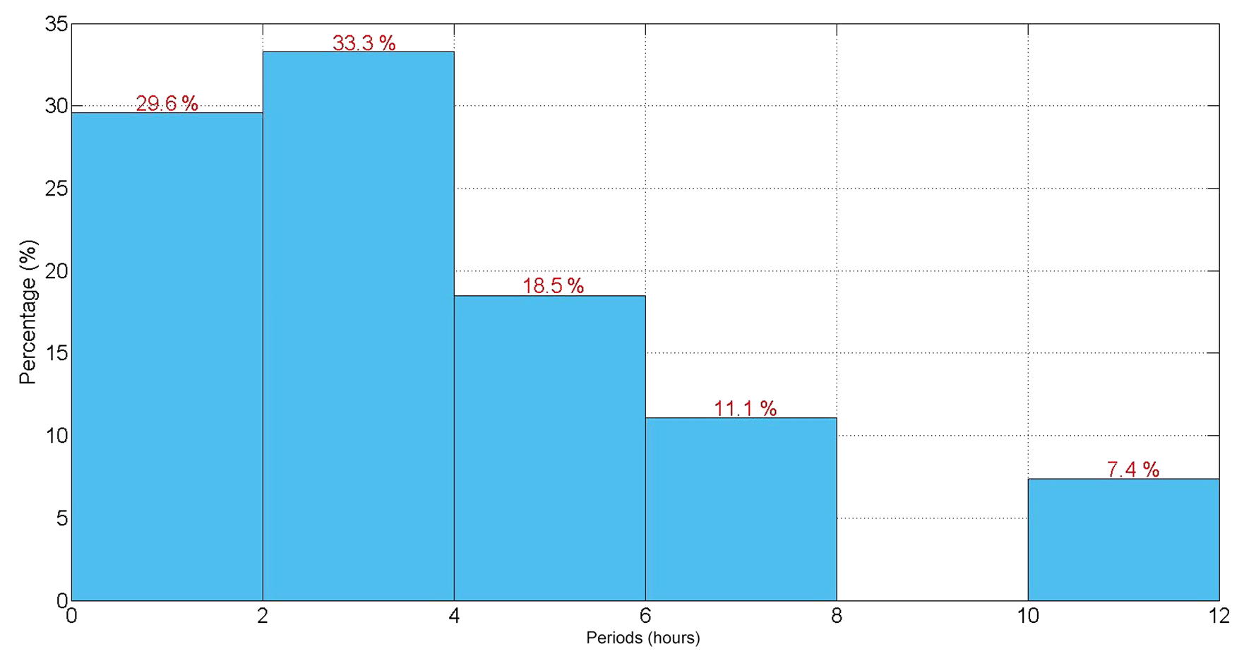
Figure 7Histogram with the periods of highest correlations between IMF Bz component and Bx geomagnetic component.
This interval corresponds to the periods observed by Echer et al. (2017) during HSS for the intervals from 19 to 20 September and 15 to 16 October 2003. In that work periods from 1.8 up to 3.1 h were found in the cross wavelet analysis between the ACE IMF Bz component and Cluster tail Bx geomagnetic field component. The periods analyzed by Echer et al. (2017) include the HILDCAA events number 2 and 3 listed in Table 1.
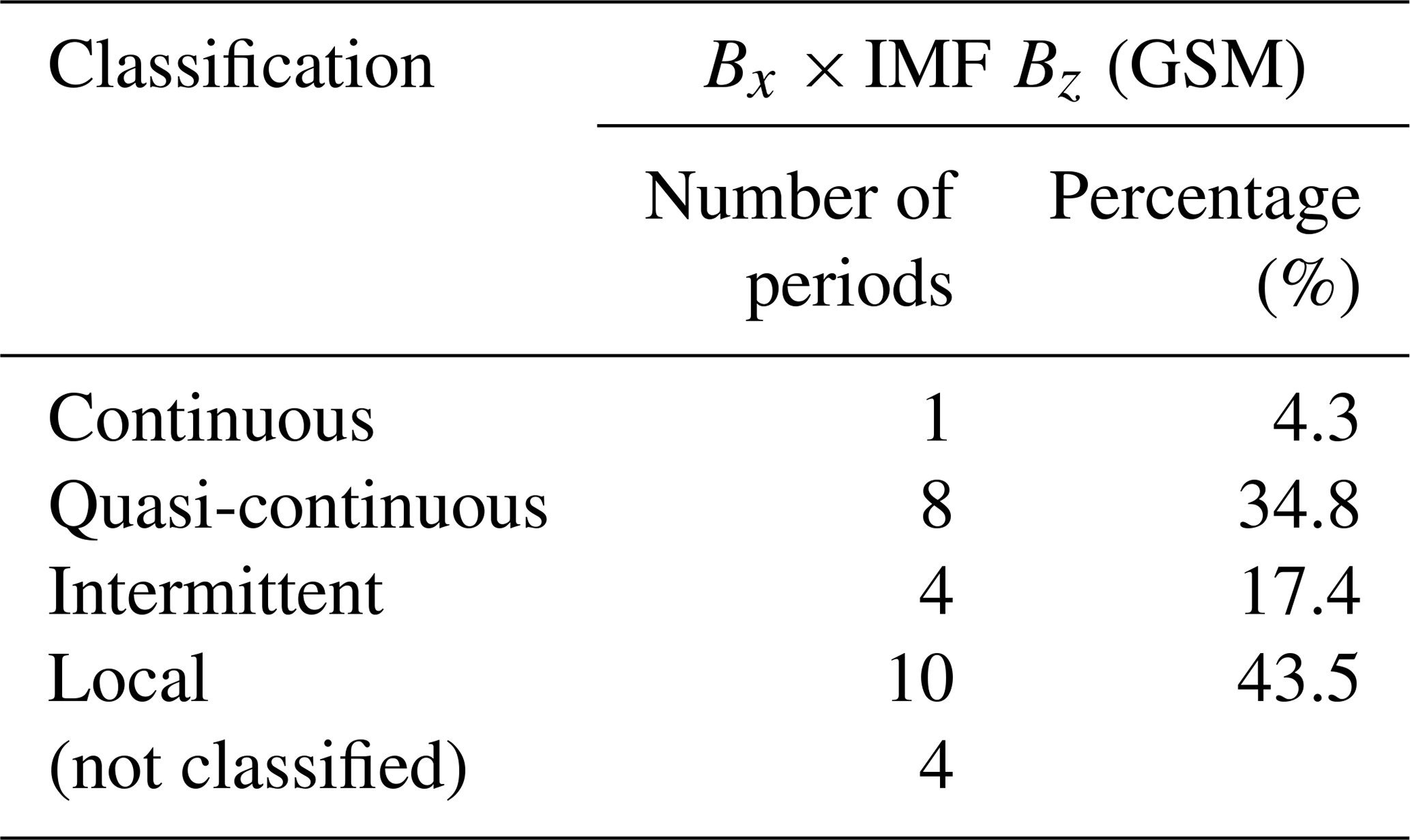
The correlation distribution form was also classified with the criteria used in the energy distribution of the Bx geomagnetic component. The result of this study is shown in Table 3. From the 27 periods with higher correlation values, 4 periods did not present a clear behavior and they were not included in the classification analysis. The local distribution was the most observed here, present in 43.5 % of the periods with higher correlation obtained. These results show that in this study, more than 95 % of coupling between the IMF Bz component and geomagnetic magnetotail Bx component is of the non-continuous type. This result is typical substorm intermittent behavior.
Table 3Correlation distribution characteristics between IMF Bz andeomagnetic Bx g component during HILDCAAs.
4.3 Energy transfer from magnetotail to auroral region during HILDCAA events
With the aim of verifying at which frequencies the transfer of the magnetotail-stored energy to the auroral region occurs during HILDCAAs, as it was observed before for other kinds of geomagnetic activity such as substorms (Hargreaves, 1992; Korth et al., 2006), the CWT was applied between the Bx geomagnetic field tail component and the AE index. Figure 8 shows the CWT applied on event 1 from Table 1. In Fig. 8a Bx and AE time series are shown. In Fig. 8b the CWT can be observed. Looking at Fig. 8b, it is possible to note that there is a high correlation in some periods, one of them for almost the whole event. The type of distributions of the correlation is also shown in the figure, which is local and quasi-continuous. In the global correlation spectrum, presented in Fig. 8c, two peaks of the periods of high values of correlation are observed at 3.7 h and at 5.6 h, respectively.
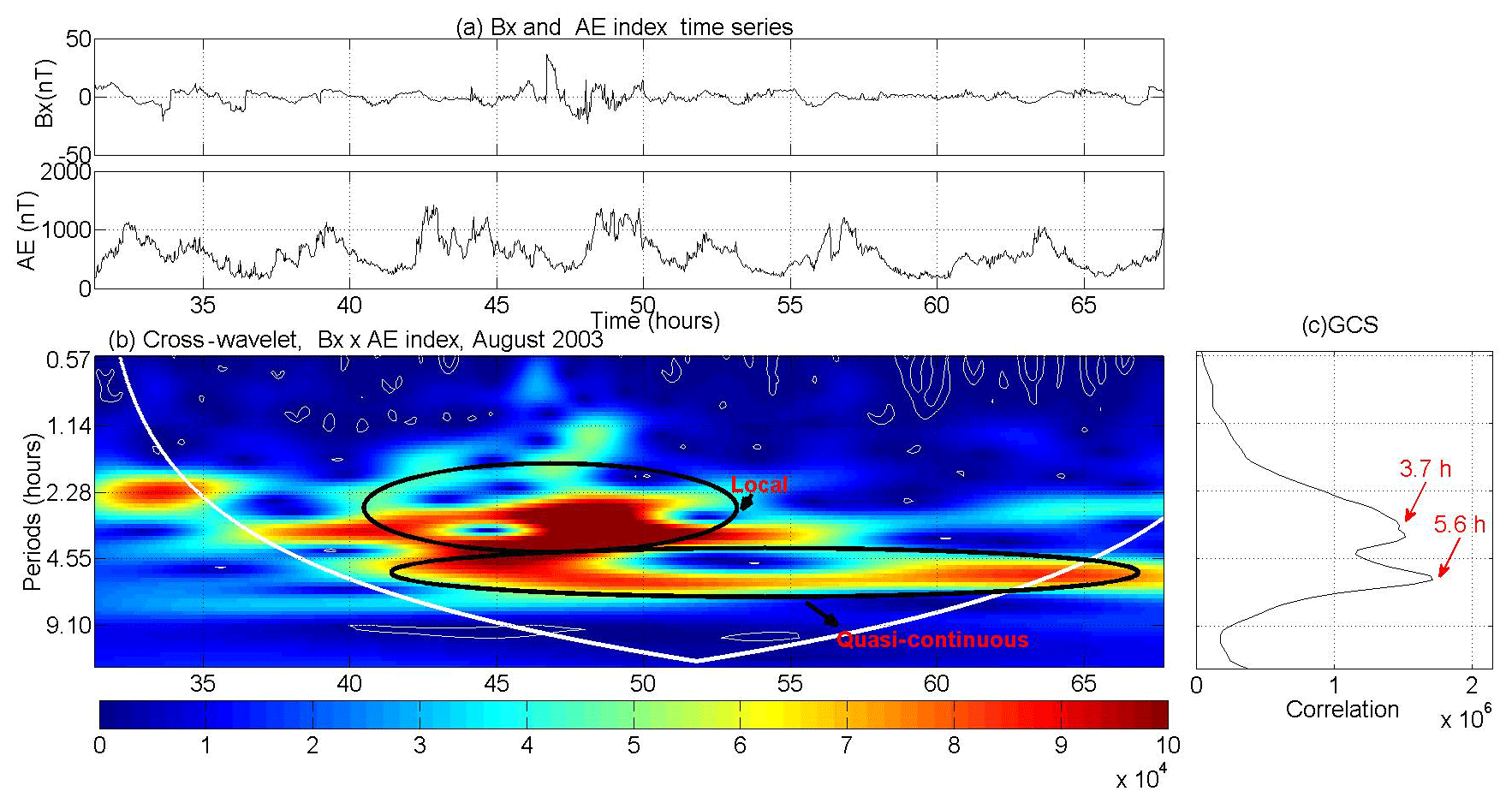
Figure 8(a) Filtered Bx geomagnetic magnetotail component and AE index time series. (b) CWT for the HILDCAA event that occurred between 15:11 UT on 20 August, and 15:43 UT on 24 August 2003. (c) Global correlation spectrum. In (a) and (b), the x axes represent the number of hours after the HILDCAA event started.
Similar analysis was also done for the whole data set and a histogram with the periods of high correlation was built, as shown in Fig. 9. From the results shown in this histogram it is possible to observe that the major periods of correlation are ≤12 h. Those were divided into 6 intervals of 2 h. Among them, one can notice that the highest correlation occurs in periods between 2 and 4 h, since 45 % of the 20 periods identified are in this range. This result is interesting and means that the energy transfer from the magnetotail to the auroral regions occurs mainly during HILDCAA-induced fluctuations with periods between 2 and 4 h.
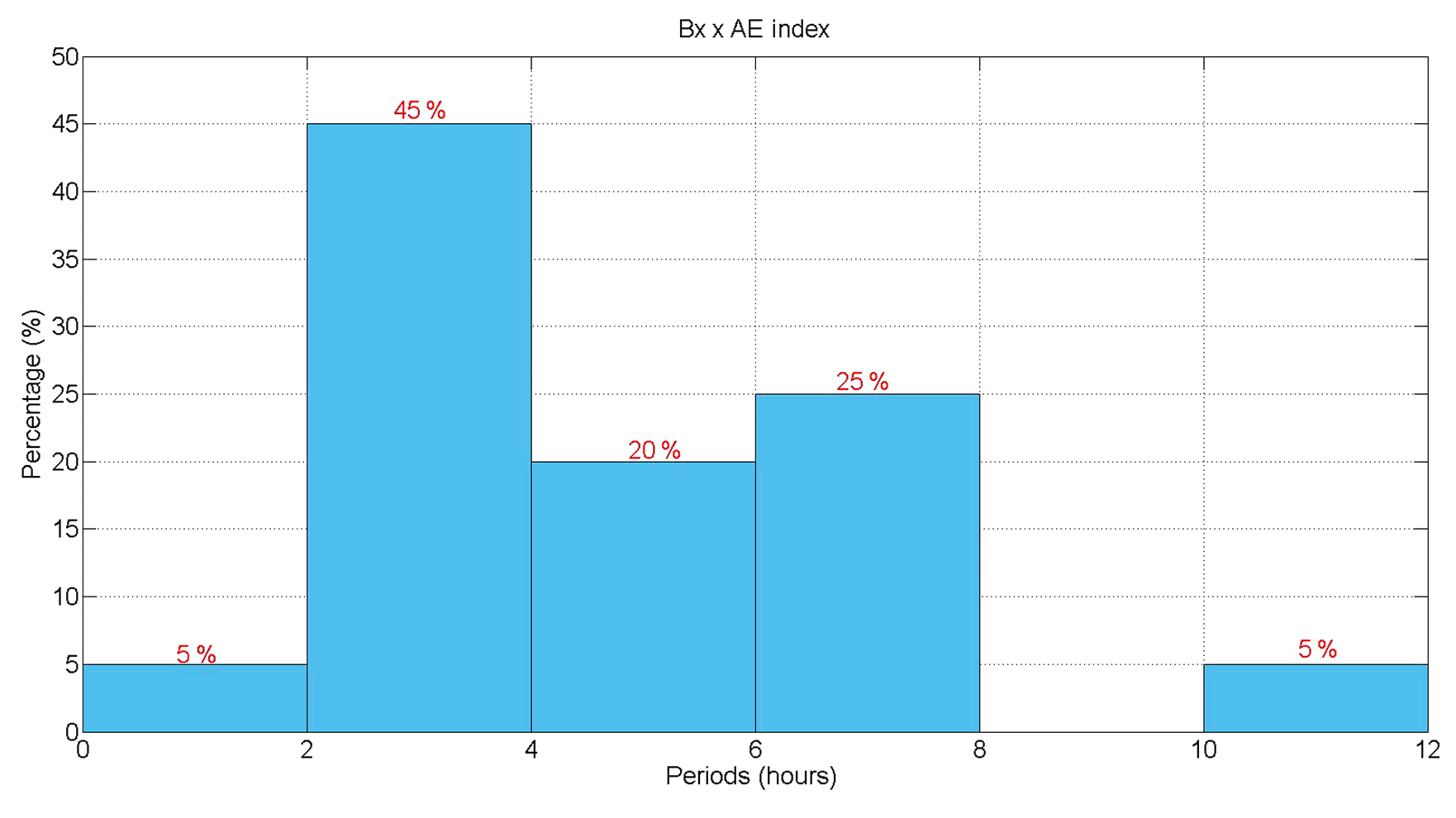
Figure 9Histogram with the periods of high correlation between Bx tail component and the AE index.
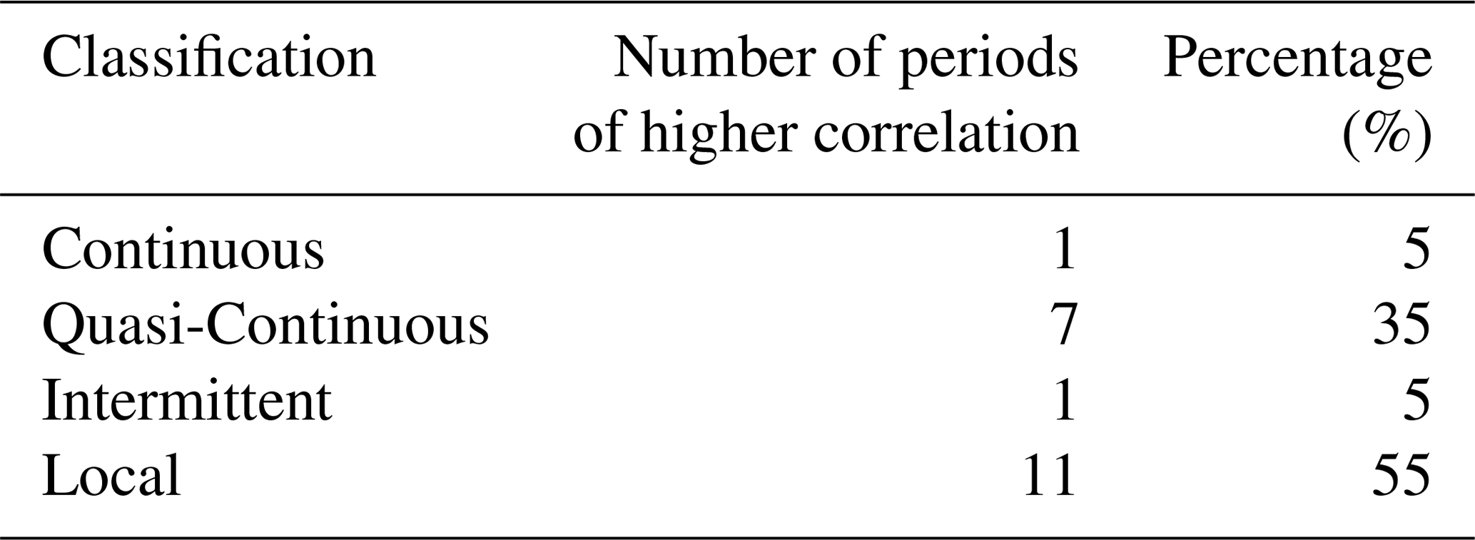
The classification of the correlation distribution was done following the steps of the analysis described previously. By this analysis, the most common correlation distribution types observed were local, present in 55 % of the main periods. This result is shown in Table 4.
Table 4Classification of the correlation distribution type between geomagnetic tail field Bx component and AE index During HILDCAAs.
In this study the main periodicities in the Bx magnetotail component and also the periodicities at which higher correlations were recorded between the IMF Bz component and Bx geomagnetic field tail component, and between Bx geomagnetic field tail component and AE index were determined. This analysis provides the frequencies where stronger energy coupling and modulation of the magnetotail by the IMF Bz variations during HILDCAAs can be observed. The periods that were found in our results agree with what was found by other authors (Lee et al., 2006; Korth et al., 2006; Bolzan et al., 2012; Echer et al., 2017): where periods of ≤4 h were identified, these periods can be associated with quasi-periodic response to solar wind forcing in the magnetotail and auroral regions, during HILDCAA events, where multiple energy injections in the magnetosphere occur, as was observed in the energy distribution analysis.
The main goal of this paper was to identify the main periods of HILDCAA events in the magnetotail, as well as to find the major periods of energy transfer from solar wind to the magnetotail and also from the magnetotail to the auroral region. The main results obtained here were as follows
The most energetic periods were observed for T≤4 h in the Bx component in the magnetotail during HILDCAAS. This result is coincident with cyclic substorm periods observed by Korth et al. (2006).
The characteristic periods of energy transfer from solar wind to the magnetotail observed in the XWT were also observed mainly for ≤4 h, in 62.9 % of the identified periods. Echer et al. (2017) also found similar periods in the study of periods of HSS-storm- and substorm-driven events in the magnetotail.
The energy transfer process between magnetotail and auroral region during HILDCAA events has also been shown to be more efficient in periods between 2 and 4 h, with 45 % of the periods identified using XWT analysis. The correlation between the Bx geomagnetic field component and the AE index is higher for the local type of distribution, which means that the energy transfer should preferentially occur in localized regions in the magnetotail or due to a short, burst-like event in the tail.
Therefore, this work presented some characteristics of HILDCAA events in the magnetotail, which were shown to be consistent with results found by other authors studying substorm- and HSS-storm-driven events, which are related to HILDCAA occurrence. Thus the magnetotail responds stronger to IMF fluctuations during HILDCAAS at 2–4 h scales, which are typical substorm periods. These results indicate that energy transfer from solar wind to magnetosphere during HILDCAA events occurs preferentially through intermittent magnetic reconnection between the fluctuating IMF Bz field and Earth's magnetopause diurnal fields, at timescales of 2–4 h. This scale is most likely the high-speed stream Alfvén wave main oscillation periods that affect Earth's magnetosphere.
The AE index, IMF Bz and Cluster Bx data used in this paper are publicly available at http://wdc.kugi.kyoto-u.ac.jp/dstae/index.html (WDC, 2019), https://csa.esac.esa.int/csa-web/\#search (ESA, 2019) and https://omniweb.gsfc.nasa.gov/form/sc_merge_min1.html (GSFC, 2019).
EE conceived the idea. MJAB developed and provided the long-term trends removal code. AMSF performed the data analysis. AMSF and EE analyzed and finalized the results after discussion with all authors. AMSF prepared the paper with contributions from all authors. All authors discussed and revised the paper.
The authors declare that they have no conflict of interest.
This article is part of the special issue “7th Brazilian meeting on space geophysics and aeronomy”. It is a result of the Brazilian meeting on Space Geophysics and Aeronomy, Santa Maria/RS, Brazil, 5–9 November 2018.
Adriane Marques de Souza Franco, Mauricio José Alves Bolzan and Ezequiel Echer would like to thank FAPESP agency, CNPq and FAPEG for their support.
Adriane Marques de Souza Franco was supported by the FAPESP agency (projects 2016/10794-2 and 2017/00516-8) and CNPq (project 300234/2019-8). Mauricio José Alves Bolzan was supported by FAPEG (grant no. 201210267000905) and CNPq (grants no. 303103/2012-4). Ezequiel Echer was supported by the CNPq (project CNPq/PQ 302583/2015-7) and FAPESP (project 2018/21657-1).
This paper was edited by Inez Batista and reviewed by Rajkumar Hajra and one anonymous referee.
Addison, P. S.: Introduction to redundancy rules: the continuous wavelet transform comes of age, Philos. T. R. Soc. A, 376, 20170258, https://doi.org/10.1098/rsta.2017.0258, 2018.
Akasofu, S.-I.: The development of the auroral substorm, Planet Space Sci., 12, 273–282, 1964.
Akasofu, S.-I.: Energy coupling between the solar wind and the magnetosphere, Space Sci. Rev., 28, 121–190, 1981.
Akasofu, S.-I.: The relationship between the magnetosphere and magnetospheric/auroral substorms, Ann. Geophys., 31, 387–394, https://doi.org/10.5194/angeo-31-387-2013, 2013.
Axford, W. I. and Hines, C. O.: A unifying theory of high latitude geophysical phenomena and geomagnetic storms, Can. J. Phys., 39, p. 1433, 1961.
Balogh, A., Carr, C. M., Acuña, M. H., Dunlop, M. W., Beek, T. J., Brown, P., Fornaçon, K.-H., Georgescu, E., Glassmeier, K.-H., Harris, J., Musmann, G., and Oddy, T: The Cluster Magnetic Field Investigation: overview of in-flight performance and initial results, Ann. Geophys., 19, 1207–1217, 2001.
Bolzan, M. J. A., Guarnieri, L. F., and Vieira, P. C.: Comparisons between two wavelet functions in extracting coherent structures from solar wind time series, Braz. J. Phys., 39, 14–17, 2009.
Bolzan, M. J. A., Echer, E., and Korth, A.: Cross-wavelet analysis on the interplanetary and magnetospheric tail magnetic field data, in: Congresso Nacional de Matemática Aplicada e Computacional (SBMAC), Vol. 34, Águas de Lindóia, São Paulo, 797–802, 2012.
Bolzan, M. J. A., Franco, A. M. S., and Echer, E.: A wavelet based method to removal of the long term trend periodicities present in geophysical time series, submitted, 2019.
Borovsky, J. E., Nemzek, R. J., and Belian, R. D.: The occurrence rate of magnetospheric substorm onsets: Random and period substorms, J. Geophys. Res., 98, 3807–3813, 1993.
Daubechies, I.: Ten lectures on wavelets, IN: Series: Cbms-Nsf Regional Conference Series In Applied Mathematics, 61, Philadelphia, Proceedings, ISBN 0898712742, 1992.
Dungey, J. W.: Interplanetary magnetic field and the auroral zones, Phys. Rev. Lett., 6, 47–49, 1961.
Echer, E., Korth, A., Bolzan, M. J. A., and Friedel, R. H. W.: Global geomagnetic responses to the IMF Bz fluctuations during the September/October 2003 high-speed stream intervals, Ann. Geophys., 35, 853–868, https://doi.org/10.5194/angeo-35-853-2017, 2017.
ESA: Cluster Science Archive, available at: https://csa.esac.esa.int/csa-web/#search, last access: 7 October 2019.
Gonzalez, W. D., Joselyn, J. A., Kamide, Y., Kroehl, H. W., Rostoker, G., Tsurutani, B. T., and Vasyliunas, V. M.: what is a geomagnetic storm?, J. Geophys. Res., 99, 5771–5792, 1994.
Grinsted, A., Moore, J. C., and Jevrejeva, S.: Application of the cross wavelet transform and wavelet coherence to geophysical time series, Nonl. Process. Geophys., 11, 561–566, 2004.
GSFC: 1-min Solar Wind data shifted to bowshock nose: plots and lists, available at: https://omniweb.gsfc.nasa.gov/form/sc_merge_min1.html, last access: 8 October 2019.
Guarnieri, F. L.: Estudo da origem interplanetária e solar de eventos de atividade auroral contínua e de longa duração, (INPE-13604-TDI/1043), Doctoral Thesis, National Institute for Space Research, São José dos Campos, 316 pp., 2005.
Guarnieri, F. L.: The nature of auroras during high-intensity long-duration continuous AE activity (HILDCAA) events, 1998 to 2001, in: Recurrent magnetic storms: corotating solar wind streams, edited by: Tsurutani, B. T., Mcpherron, R. L., Gonzalez, W. D., Lu, G., Sobral, J. H. A., Gopalswamy, N., Geophys. Monogr., Washington, DC, Am. Geophys. Univ. Press., 167, 235–243, 2006.
Haar A.: Zur Theorie der orthogonalen Funktionensysteme, Math. Ann., 69, 331–371, 1910.
Hajra, R., Echer, E., Tsurutani, B. T., and Gonzalez, W. D.: Solarwind-magnetosphere energy coupling efficiency and partitioning: HILDCAAs and preceding CIR storms during solar cycle 23, J. Geophs. Res., 119, 2675–2690, 2014.
Hargreaves, J. K.: Solar-terrestrial environment an introduction to geospace – the science of the terrestrial upper atmosphere, ionosphere and magnetosphere – Cambridge, UK, Cambridge University, 1992.
Hones, E. W. Jr.: Transient Phenomena in the Magnetotail and their Relation to Substorms, Space Sc. Revi., 23, 393–410, 1979.
Korth, A., Echer, E., Guarnieri, F. L., Franz, M., Friedel, R., Gonzalez, W. D., Mouikis, C. G., and Reme, H.: Cluster observations of plasma sheet activity during the 14–28 September 2003 corotating high speed stream event, in: Proceedings of the Eight Interna-tional Conference on Substorms (ICS-8), edited by: Syrjäsuo, A. and Donovan, E., University of Calgary, 133–138, 2006.
Lee, D. Y., Lyons, L. R., Kim, K. C., Baek, J. H., Kim, K. H., Kim, H. J., Weygand, J., Moon, Y. J., Cho, K. S., Park, Y. D., and Han, W.: Repetitive sub storms caused by Alfvénic waves of the interplanetary magnetic field during high – speed solar wind streams, J. Geophys. Res., 111, 1–14, 2006.
Lopez, R.: Magnetospheric substorms, Johns Hopkins APL Technical Digest, 11, 264–271, 1990.
Mendes, O., Domingues, M. O., Echer, E., Hajra, R., and Menconi, V.: Characterization of high-intensity, long-duration continuous activity (HILDCAA) events using recurrence quantification analysis, Nonl. Process. Geophys., European Geosciences Union (EGU), 24, 407–417, 2017.
Morettin, P. A.: Ondas e ondeletas: da análise de fourier à análise de ondeletas, São Paulo, Edusp, 296 pp., 1992.
Porwik, P. and Lisowska, A.: The Haar–Wavelet Transform in Digital Image Processing: Its Status and Achievements, Machine Graphics & Vision, 13, 79–98, 2004.
Sitnov, M. I., Sharma, A. S., Papadopoulos, K., and Vassiliadis, D.: Modeling substorm dynamics of the magnetosphere: from self-organization and self-organized criticality to nonequilibrium phase transitions, Phys. Rev. E, 65, 016116, https://doi.org/10.1103/PhysRevE.65.016116, 2001.
Smith E. J., Balogh, A., Neugebauer, M., and Mccomas, D.: Ulysses observations of Alfvén waves in the southern and northern solar hemispheres, Geophys. Res. Lett., 22, 3381–3384, 1995.
Souza, A. M., Echer, E., Bolzan, M. J. A., and Hajra, R.: A study on the main periodicities in interplanetary magnetic field Bz component and geomagnetic AE index during HILDCAA events using wavelet analysis, J. Atmos. Sol.-Terr. Phys., 149, 81–86, 2016.
Souza, A. M., Echer, E., Bolzan, M. J. A., and Hajra, R.: Cross-correlation and cross-wavelet analyses of the solar wind IMF Bz and auroral electrojet index AE coupling during HILDCAAs, Ann. Geophys., 36, 205–211, https://doi.org/10.5194/angeo-36-205-2018, 2018.
Torrence, C. and Compo, G. P.: A practical guide to wavelet analysis, Bull. Am. Meteorol. Soc., 79, 61–78, 1998.
Tsurutani, B. T. and Gonzalez, W. D.: The Cause Of High-Intensity Long-Duration Continuous AE Activity (Hildcaas): Interplanetary Alfven Wave Trains. Planet. Space Sci., 35, 405–412, 1987.
Tsurutani, B. T., Gould, T., Goldstein, B. E., Gonzalez, W. D., and Sugiura, M.: Interplanetary Alfven waves and auroral (substorm) activity: IMP-8, J. Geophys. Res., 95, 2241–2252, 1990.
Tsurutani, B. T., Gonzalez, W. D., Guarnieri, F. L., Kamide, Y., Zhou, X., and Arballo, J. K.: Are high-intensity long-duration continuous AE activity (HILDCAA) events substorm expansion events?, J. Atmos. Sol.-Terr. Phys., 66, 67–176, 2004.
WDC: Plot and data output of Dst and AE indices, available at: http://wdc.kugi.kyoto-u.ac.jp/dstae/index.html, last access: 8 October 2019.