An improved pixel-based water vapor tomography model

As an innovative use of Global Navigation Satellite System (GNSS), the GNSS water vapor tomography technique shows great potential in monitoring three-dimensional water vapor variation. Most of the previous studies employ the pixel-based method, i.e., dividing the troposphere space into finite voxels and considering water vapor in each voxel as constant. However, this method cannot reflect the variations in voxels and breaks the continuity of the troposphere. Moreover, in the pixel-based method, each voxel needs a parameter to represent the water vapor density, which means that huge numbers of parameters are needed to represent the water vapor field when the interested area is large and/or the expected resolution is high. In order to overcome the abovementioned problems, in this study, we propose an improved pixel-based water vapor tomography model, which uses layered optimal polynomial functions obtained from the European Centre for Medium-Range Weather Forecasts (ECMWF) by adaptive training for water vapor retrieval. Tomography experiments were carried out using the GNSS data collected from the Hong Kong Satellite Positioning Reference Station Network (SatRef) from 25 March to 25 April 2014 under different scenarios. The tomographic results are compared to the ECMWF data and validated by the radiosonde. Results show that the new model outperforms the traditional one by reducing the root-mean-square error (RMSE), and this improvement is more pronounced, at 5.88 % in voxels without the penetration of GNSS rays. The improved model also has advantages in more convenient expression.

1 Introduction

As the most active component in the troposphere, water vapor is one of the most difficult parameters to monitor and describe (Rocken et al., 1997). A good understanding of the spatio-temporal variation of water vapor is very helpful for improving weather forecasting and early warning of disastrous weather (Weckwerth et al., 2004).

The Global Navigation Satellite System (GNSS) technique can not only retrieve the precipitable water vapor (Bevis et al., 1994; Emardson et al., 1998; Baltink et al., 2002; Bock et al., 2005) but can also monitor the three-dimensional water vapor distribution by using the GNSS tomography method (Flores et al., 2000; Seko et al., 2000; Macdonald et al., 2002).

Braun et al. (1999) first proposed the concept of reconstructing the tropospheric water vapor structure using 20 GPS stations in a regional observational network. Flores et al. (2000) first applied the tomography technique to obtain wet refractivity from the GNSS slant wet delay (SWD). In the same year, Hirahara (2000) used a different method to conduct GNSS tomography experiments, which also successfully obtained three-dimensional water vapor fields. Since then, many scientists proposed new methods and applied them to GNSS water vapor tomography experiments (Rohm et al., 2014; Yao et al., 2016; Zhang et al., 2017; Ding et al., 2018; Zhao et al., 2018).

Hirahara (2000) conducted a four-dimensional tomography experiment and solved the tomography equations using the damped least-squares method. Braun et al. (2003) and Braun (2004) overcame the sensitivity problem in GNSS tomography by using the extended sequential filtering method. Perler et al. (2011) presented a new parametric method for the water vapor retrieval. Nilsson and Gradinarsky (2006) obtained the wet refractivity directly from the GNSS-phase observations using the Kalman filter method. Rohm and Bosy (2009) used the Moore–Penrose pseudo-inverse of variance and covariance to solve the linear equations and emphasized the ill-posed tomography equation. Yao et al. (2016) obtained good tomographic results by using the optimal grid-making method. Zhao and Yao (2017) proposed a method of using the side-penetrating signals for tomography and improved the utilization rate of the GNSS rays. Aghajany and Amerian (2017) obtained the tomography results of water vapor profiles from ERA-I numerical weather prediction data by applying a 3-D ray tracing technique. Dong and Jin (2018) reconstructed the water vapor density using multi-GNSS systems and showed that the accuracy of GNSS tomography results are improved by 5 % from the GPS-only system to the dual systems (GPS + GLONASS). Besides, the virtual reference station approach (Marel, 1998; Vollath et al., 2013), an effective method for attenuating the effects of atmospheric errors in long-distance dynamic positioning, was also used in GNSS tropospheric tomography.

In previous studies, since most of the GNSS tomography methods divided the troposphere of interest into finite voxels, and the water vapor density in each voxel is considered as constant, these methods with the above assumptions are defined as the pixel-based method. Apparently, this kind of method cannot retrieve the variations in voxels and breaks the continuous nature of the troposphere as well. Moreover, the pixel-based method requires each voxel to have a parameter to represent the water vapor density in it, which may lead to the situation that we have to use huge numbers of parameters when the research area is large and the expected resolution is high. Last, over-parameterization may cause mathematical problems when we use limited observations to invert for the parameters that may be correlated. Therefore, this paper analyzes the limitations of the traditional pixel-based water vapor tomography method and proposes an improved model. The improved model uses the water vapor density obtained from the traditional model as the input value and outputs the fitting water vapor density by the layered optimal polynomial functions. This new model has the advantage of reflecting the variations in voxels and keeping the continuity of water vapor in the troposphere.

2 An improved pixel-based water vapor tomography model

2.1 Establishment of the traditional pixel-based water vapor tomography model

2.1.1 Retrieval of SWV

For tropospheric tomography, the most important observation is the slant water vapor (SWV), which is related to the water vapor density and can be defined by

$$\begin{array}{}\text{(1)}& \mathrm{SWV}=\underset{S}{\int }{\mathit{\rho }}_{\mathrm{V}}\mathrm{d}s,\end{array}$$

where s represents the path of the satellite signal ray, and ρ_V is the water vapor density (units: g m⁻³). SWV can be obtained by the following method:

$$\begin{array}{}\text{(2)}& \mathrm{SWV}={\displaystyle \frac{{\mathrm{10}}^{\mathrm{6}}}{R_{\mathit{\omega }}\left[\right(k_{\mathrm{3}}/T_{\mathrm{m}})+k_{\mathrm{2}}^{\prime }]}}\cdot \mathrm{SWD},\end{array}$$

where $k_{\mathrm{2}}^{\prime }=\mathrm{16.48}$ K hPa⁻¹, $k_{\mathrm{3}}=\mathrm{3.776}\times {\mathrm{10}}^{\mathrm{5}}$ K² hPa⁻¹, and R_ω=461 J kg⁻¹ K⁻¹, which represent the specific gas constants for water vapor. T_m is the weighted mean tropospheric temperature, calculated from an empirical equation proposed by Liu et al. (2001) using the meteorological measurements. SWD is the slant wet delay, which may be given as

$$\begin{array}{ll}{\displaystyle }& {\displaystyle }{\mathrm{SWD}}_{\mathrm{elv},\mathit{\phi }}=m_{\mathrm{wet}}\left(\mathrm{elv}\right)\times \mathrm{ZWD}+m_{\mathrm{wet}}\left(\mathrm{elv}\right)\times \cot \left(\mathrm{elv}\right)\\ \text{(3)}& {\displaystyle }& {\displaystyle }\times (G_{\mathrm{NS}}^{\mathrm{w}}\times \cos \mathit{\phi }+G_{\mathrm{EW}}^{\mathrm{w}}\times \sin \mathit{\phi })+R,\end{array}$$

where elv is the satellite elevation, φ is the azimuth, m_wet is the wet mapping function, and $G_{\mathrm{NS}}^{\mathrm{w}}$ and $G_{\mathrm{EW}}^{\mathrm{w}}$ are the wet delay gradient parameters in the north–south and east–west directions, respectively. R refers to the non-modeled zero difference residuals that may involve unmodeled influence on the three-dimensional spatial water vapor distribution, which can make up for the lack of tropospheric anisotropy using only the gradient term (Bi et al., 2006). Since the GAMIT software only provides the double difference residuals, the zero difference residuals in this paper are obtained from the double difference residuals according to the method proposed by Alber et al. (2000). ZWD is the zenith wet delay, which is extracted from the zenith tropospheric delay (ZTD) by separating the zenith hydrostatic delay (ZHD) using equation ZWD = ZTD − ZHD. ZHD can be calculated precisely using surface pressure based on the Saastamoinen model (Saastamoinen, 1972):

$$\begin{array}{}\text{(4)}& \mathrm{ZHD}={\displaystyle \frac{\mathrm{0.002277}\times P_{\mathrm{s}}}{\mathrm{1}-\mathrm{0.00266}\times \cos \left(\mathrm{2}\mathit{\phi }\right)-\mathrm{0.00028}\times H}},\end{array}$$

where P_s is the surface pressure (unit: hPa), φ is the latitude of the station, and H is the geodetic height (unit: km). The unit of ZHD is meter.

Since the SWV is obtained, the tomographic area can be discretized into a number of voxels in which the water vapor density is a constant during a given period of time. Therefore, a linear equation relating the SWV and the water vapor density can be established as follows (Chen and Liu, 2014):

$$\begin{array}{}\text{(5)}& {\mathrm{SWV}}^p=\sum _{ijk}(D_{ijk}^{\mathrm{p}}\cdot {\mathit{\rho }}_{ijk}),\end{array}$$

where SWV^p is the slant water vapor of ρth signal path (unit: mm). i, j, and k are the positions of discrete tomographic voxels in the longitudinal, latitudinal, and vertical directions, respectively. $D_{ijk}^{\mathrm{p}}$ is the distance of the ρth signal in voxel (i, j, k; unit – km). ρ_ijk is the water vapor density in a given voxel (i, j, k; unit – g m⁻³). A matrix form of this observation equation can be rewritten as follows (Flores et al., 2000; Chen and Liu, 2014):

$$\begin{array}{}\text{(6)}& y_{m\times \mathrm{1}}={\mathbf{A}}_{m\times n}\cdot {\mathit{\rho }}_{n\times \mathrm{1}},\end{array}$$

where m is the number of total SWVs, and n is the number of voxels in the tomographic area. y is the observed value here as the SWV, which penetrates the whole interest area, A is the coefficient matrix of the signal transit distances through the voxels, and ρ is the column vector of the unknown water vapor density.

2.1.2 Constraint equations of the tomography modeling

Solving for the unknown water vapor density in Eq. (6) is actually an inversion algorithm issue, as the design matrix A is a large sparse matrix whose normal equation is singular, leading to numerical problems when using a direct inversion method (Bender et al., 2011). To overcome this rank deficiency problem, constraint equations are often introduced into the tomography equation (Flores et al., 2000; Troller et al., 2002; Rohm and Bosy, 2009; Bender et al., 2011). In our study, the horizontal constraint equation is imposed by the Gaussian weighted functional method (Guo et al., 2016), and the vertical constraint equation is imposed by the functional relationship of the exponential distribution (Cao, 2012), respectively. The final tomography model is then obtained as

$$\begin{array}{}\text{(7)}& \left(\begin{array}{l}{\mathbf{A}}_{m\times n}\\ {\mathbf{H}}_{m\times n}\\ {\mathbf{V}}_{m\times n}\end{array}\right)\cdot {\mathit{\rho }}_{n\times \mathrm{1}}=\left(\begin{array}{l}{y}_{m\times n}\\ {\mathrm{0}}_{m\times n}\\ {\mathrm{0}}_{m\times n}\end{array}\right),\end{array}$$

where H and V are the coefficient matrices of horizontal and vertical constrains, respectively. In order to obtain the inverse matrix shown in Eq. (7), singular value decomposition is used in this paper (Flores et al., 2000).

2.2 An improved pixel-based water vapor tomography model

The improved pixel-based water vapor tomography model proposed in this paper can take advantage of facilitating the continuity of the water vapor expression efficiently in spatio-temporal distribution and calculating the water vapor density conveniently. The improved tomography model firstly obtains the water vapor density from voxels penetrated by GNSS rays using the traditional pixel-based tomography model then obtains the optimal polynomial function of each layer through adaptive training. With known coefficients of the layered optimal polynomial functions, the water vapor density can finally be calculated given the latitude, longitude and the altitude. Specific steps are as follows.

First, use the traditional pixel-based water vapor tomography model to obtain the initial water vapor density from voxels penetrated by GNSS rays as the observation values for obtaining the optimal polynomial function coefficients of each layer.

Second, normalize the coordinates of each voxel center in the tomographic area, since the polynomial fitting of the water vapor at each tomographic layer is, in essence, for establishing the relationship between the latitude as well as the longitude of the tomographic region and the water vapor density. The general expression is:

$$\begin{array}{}\text{(8)}& V_{\mathrm{d}}=a_{\mathrm{0}}+a_{\mathrm{1}}B+a_{\mathrm{2}}L+a_{\mathrm{3}}BL+a_{\mathrm{4}}{B}^{\mathrm{2}}+a_{\mathrm{5}}{L}^{\mathrm{2}}+a_{\mathrm{6}}{B}^{\mathrm{2}}L\mathrm{\dots },\end{array}$$

where B is the latitude, L is the longitude, and V_d represents the water vapor density. Polynomial coefficients such as a_i are obtained via the least-squares method. In the process of data solving, where the numerical values of the latitude and longitude may not be small, then the magnitude of multiple power may be larger than 10⁴, which will lead to the ill-posed problem of the design matrix in the inversion process and eventually affect the reliability of the estimated coefficients. To ensure the design matrix will be relatively stable in the inversion process, the latitude and longitude coordinates B and L need to be normalized. The specific methods are as follows:

$$\begin{array}{l}{B}^{\ast }={\displaystyle \frac{B-{\mathit{\mu }}_B}{{\mathit{\sigma }}_B}},\\ L^{\ast }={\displaystyle \frac{L-{\mathit{\mu }}_L}{{\mathit{\sigma }}_L}},\end{array}$$

where B^∗ and L^∗ are the normalized latitude and longitude, respectively, and B and L are the latitude and longitude in the initial region range. μ is the average value of the latitude or longitude, and σ is the standard deviation of the latitude or longitude.

Third, determine the layered optimal polynomial functions of the improved model through adaptive training.

• First, based on the size of the selected tomographic region, determine the highest polynomial fit order. In this paper, the highest polynomial fit order, chosen as 5, turns out to be generally sufficient.

• Then set the water vapor density from voxels penetrated by GNSS-signal rays as the input value and keep trying out new polynomial functions, as the optimal polynomial function of each layer is obtained by adaptive training. What needs to be noted here is that the number of estimated coefficients needs to be less than that of the voxels penetrated by GNSS rays in each layer. Otherwise the over-fitting problem will happen.

• Finally, after comparing training results of multi-group polynomial functions at different levels, the polynomial function with the minimum root-mean-square error (RMSE) value obtained from the water vapor density of the post-fitting layer and that of the European Centre for Medium-Range Weather Forecasts (ECMWF) is the best fitting equation for this layer. Each layer could have the individual optimal polynomial function in general.

Fourth, after finding the optimal polynomial function of each layer in different heights, using the latitude, longitude, and altitude information in the function could obtain the three-dimensional water vapor distribution in the tomographic region. The continuous water vapor density can be easily described by broadcasting the estimated coefficients of the layered optimal polynomial functions.

2.3 The optimal polynomial selection based on adaptive training

Since the polynomial form can reflect the continuity of water vapor well and has the advantage of high-efficiency computing as well as easy expression, this paper chooses the polynomial form as the layered fitting function. Based on adaptive training, the selection process of the layered optimal polynomial function is as follows.

First, construct a polynomial equation training library, which contains a wide variety of polynomial function forms of the latitude and longitude as independent variables while using the water vapor density in the voxels as the dependent variable. After many experiments, the maximum power of the latitude and longitude, found as 5, is sufficient in describing the water vapor changes. Therefore, the maximum power of the fitting function part is adopted as 5 in the training library.

Second, according to the water vapor density observations from the voxels penetrated by the GNSS signals at each level, the form of the candidate polynomial function of each layer is automatically determined from the polynomial function training library, ensuring that the number of observations at all levels is always greater than that of estimated coefficients of candidate polynomials.

Third, calculate the water vapor variation index (WVVI) of each layer in both east–west and north–south directions using the traditional water vapor tomography results as shown in Eq. (10):

$$\begin{array}{}\text{(10)}& \mathrm{WVVI}={\displaystyle \frac{\stackrel{\mathrm{‾}}{\mathrm{\nabla }w{v}_{\mathrm{EW}}}}{\stackrel{\mathrm{‾}}{\mathrm{\nabla }w{v}_{\mathrm{NS}}}}},\end{array}$$

where wv_EW and wv_NS are the water vapor density in east–west and north–south directions, respectively.

The WVVI is a changing rate indicator of the water vapor density in a given direction. According to the water vapor variation index of each layer in the east–west and north–south direction, whether the water vapor exists mainly in the east–west distribution or the north–south distribution can be determined. As an aid, WVVI can decide the main body of the alternative polynomial function with higher order, whether in longitude or latitude, and then efficiently find the layered optimal polynomial function. If the water vapor density of a layer indicates a horizontal gradient of east–west distribution, the polynomial function with higher-order term of the longitude should be given the priority. It suggests that when the water vapor shows an east–west gradient distribution, there is a better correlation between the longitude and the water vapor variation; furthermore the high-order term in longitude can better reflect the nuanced water vapor variation. A simple example of the polynomial function with a higher-order term in longitude is shown in Eq. (11):

$$\begin{array}{}\text{(11)}& {\displaystyle }{V}_{\mathrm{d}}=a_{\mathrm{0}}+a_{\mathrm{1}}B+a_{\mathrm{2}}L+a_{\mathrm{3}}BL+a_{\mathrm{4}}{L}^{\mathrm{2}}+a_{\mathrm{5}}B{L}^{\mathrm{2}}+a_{\mathrm{6}}{L}^{\mathrm{3}}.\end{array}$$

Otherwise, when the water vapor density of a layer indicates a horizontal gradient of north–south distribution, the polynomial function with higher-order term of the latitude should be given priority. A simple example is shown in Eq. (12):

$$\begin{array}{}\text{(12)}& {\displaystyle }{V}_{\mathrm{d}}=a_{\mathrm{0}}+a_{\mathrm{1}}B+a_{\mathrm{2}}L+a_{\mathrm{3}}BL+a_{\mathrm{4}}{B}^{\mathrm{2}}+a_{\mathrm{5}}{B}^{\mathrm{2}}L+a_{\mathrm{6}}{B}^{\mathrm{3}}.\end{array}$$

While the distribution regularities of the water vapor density gradient are not clear or obvious, the polynomial function with the same order of the latitude and longitude can be considered as the example shown in Eq. (13):

$$\begin{array}{}\text{(13)}& V_{\mathrm{d}}=a_{\mathrm{0}}+a_{\mathrm{1}}B+a_{\mathrm{2}}L+a_{\mathrm{3}}BL+a_{\mathrm{4}}{B}^{\mathrm{2}}+a_{\mathrm{5}}{L}^{\mathrm{2}}.\end{array}$$

Fourth, the candidate polynomials of all levels screened by the WVVI gradient auxiliary information are used as the next comparative polynomials, and the required estimated coefficients of the comparative polynomial are solved according to the principle of least squares through Eq. (14) and automatically recorded into the coefficients data set. M is the matrix of the longitude and latitude, and the vector x comprises the unknown coefficients of the comparative polynomial functions as shown in Eq. (15):

$$\begin{array}{}\text{(14)}& {\displaystyle }& {\displaystyle }{V}_{\mathrm{d}}=\mathbf{M}\mathit{x},\text{(15)}& {\displaystyle }& {\displaystyle }x=\left[\begin{array}{l}{a}_{\mathrm{0}}\\ a_{\mathrm{1}}\\ \mathrm{⋮}\\ a_n\end{array}\right].\end{array}$$

Fifth, through the comparative polynomials with the estimated coefficients in each layer, the whole-voxel water vapor fitting of each layer is automatically fit with the information of the latitude and longitude. In order to obtain the RMSE, the fitting result would be compared with the ECMWF water vapor density of each layer in this period. The results are then saved to the accuracy data sets of each layer. The comparative polynomials with the estimated coefficients are constantly selected to train the fitting of the layered water vapor density and are then compared with the water vapor density of the ECMWF at each layer. Thus, large accuracy data sets of RMSE can be obtained where the smallest RMSE value of the comparative polynomial form can be chosen, and then the optimal polynomial of each layer could come into being. It is noteworthy that the optimal polynomial of each layer might be different. With the layered optimal polynomial, the continuous three-dimensional water vapor density in the tomographic region can be expressed conveniently by transmitting the estimated coefficient's information.

3 Experiment

3.1 Experimental description and data-processing strategy

To study whether the accuracy and stability of the improved water vapor tomography model are better than those of the traditional model, the following experiment is designed.

Tomographic data are obtained from the Hong Kong Satellite Positioning Reference Station Network (SatRef) from 25 March to 25 April 2014. Two epochs are taken each day (00:00 and 12:00 UTC). The corresponding meteorological data are also used to calculate the precipitable water vapor (PWV). The tomographic area ranges between latitude 22.24 to 22.54^∘ N and longitude 113.87 to 114.29^∘ E. Taking the mean sea level as the height of the base level, the vertical resolution is 0.8 km, and the total grid number is $\mathrm{5}\times \mathrm{7}\times \mathrm{13}$. In the selected area, a total of 11 GNSS stations and one radiosonde station (located at King's Park, Hong Kong) are selected, and the ECMWF grid data are extracted twice daily, at 00:00 and 12:00 UTC, from 25 March to 25 April 2014 (grid resolution of $\mathrm{0.125}{}^{\circ }\times \mathrm{0.125}{}^{\circ }$). See Fig. 1 for details.

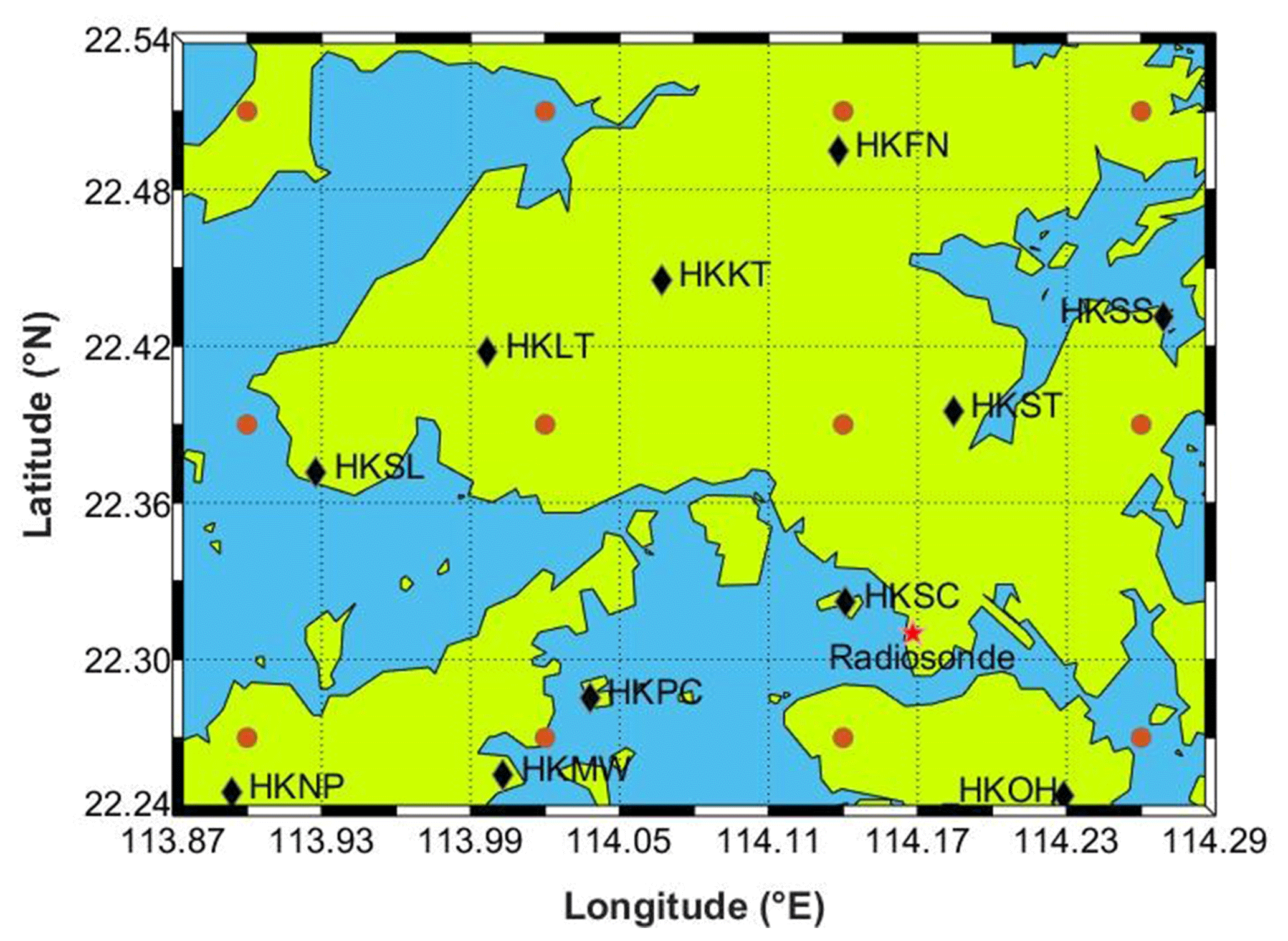
Figure 1 The GNSS stations (11 black rhombuses), the radiosonde station (one red star), and the ECMWF comparative points (12 ochre circles) in Hong Kong. The gridded lines indicate tomography grids.

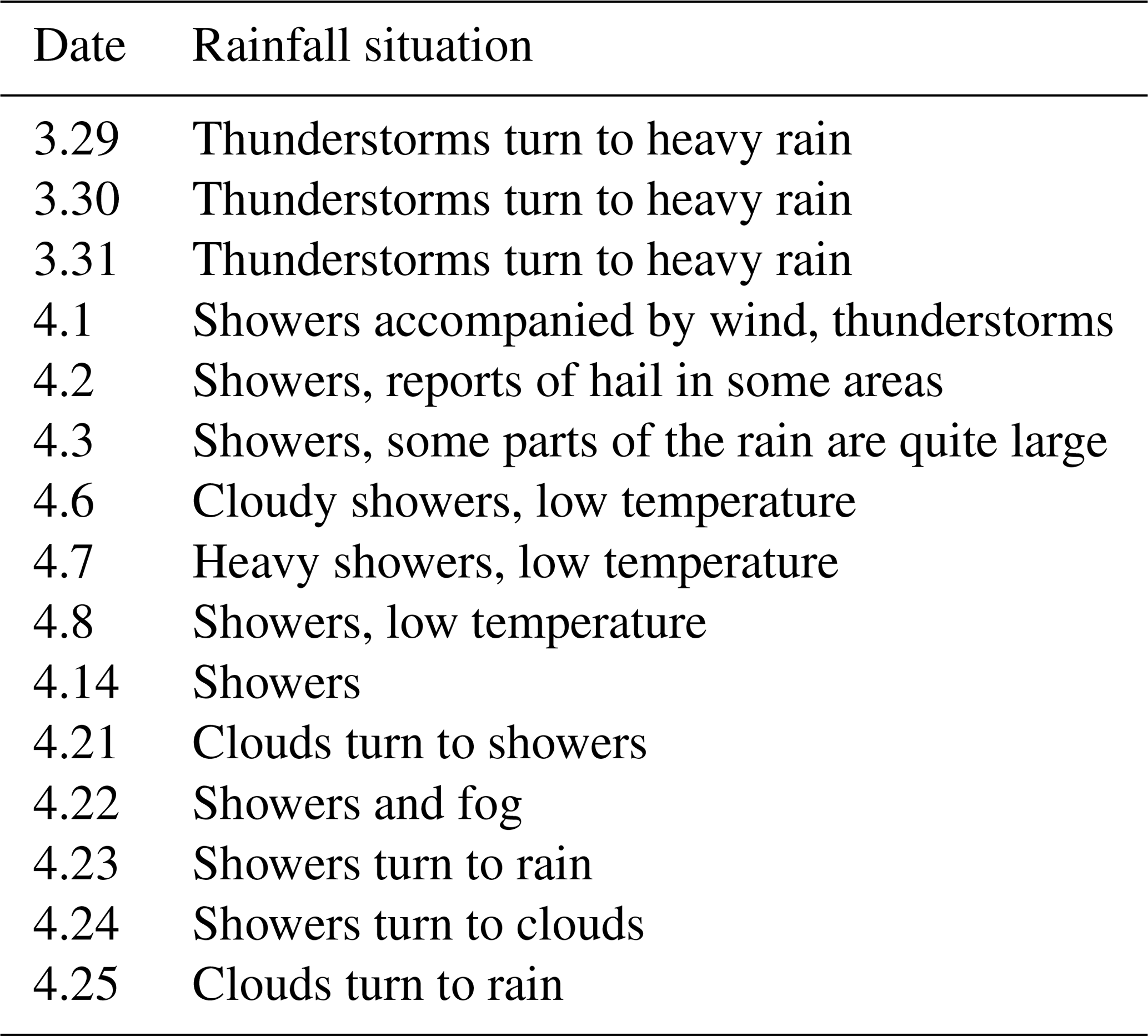
According to the official website of the Hong Kong Observatory (http://www.weather.gov.hk/wxinfo/pastwx/metob201403c.htm, last access: 30 January 2019), in the weather review, Hong Kong had a total of 15 days of rainy weather from 25 March to 25 April 2014, as shown in Table 1.

Table 1 Rainfall information for March and April 2014.

In this paper, GAMIT (v10.50; Herring et al., 2010) software was used for processing the GPS observations based on the double-differenced model at a sampling interval of 30 s, and the global mapping function was adopted. The zenith total delay (ZTD) and wet horizontal gradient intervals were estimated at 0.5 and 2 h, respectively. Based on the surface pressure obtained from observed meteorological parameters, the ZHD could be obtained by the Saastamoinen model, and ZWD was isolated from ZHD. Via GMF projection, the SWD could be obtained by transforming the observed SWV.

3.2 Experimental introduction and comparison

The RMSE and bias of the improved tomography model residuals were calculated by subtracting the ECMWF water vapor density from the water vapor density of the improved pixel-based water vapor tomography model (hereinafter referred to as the improved model). In a similar way, the RMSE and bias of the traditional tomography model residuals can also be obtained from the difference between the ECMWF water vapor density and the water vapor density obtained by the traditional pixel-based water vapor tomography model (hereinafter referred to as the traditional model).

In order to evaluate the improved model, this paper investigates six scenarios, comprising the spatial distribution scenario, the everyday distribution scenario, the rainy scenario, and the non-rainy scenario. Moreover the scenarios of residuals of the water vapor density in voxels with and without penetrating GNSS rays are inspected. The definitions of six scenarios mentioned above are as follows.

The spatial distribution scenario is investigated by obtaining the RMSE and bias of the residuals from all ECMWF comparative points at all time intervals.

The everyday distribution scenario is found by obtaining the RMSE and bias of the residuals from all ECMWF comparative points in two epochs each day. In addition the overall accuracy of 32 days between 25 March and 25 April 2014 was calculated.

The rainy scenario is based on 15 rainy days between 25 March and 25 April 2014, referred to in Table 1. The RMSE and bias of the residuals are obtained from all ECMWF comparative points for all the epochs during rainy days. Similarly, the non-rainy scenario is found with the accuracy analysis of the non-rainy days.

The scenario of residuals of the water vapor density in voxels without GNSS-ray penetration is found by obtaining the RMSE and bias of the residuals from ECMWF comparative points without rays passing through for all the epochs each day. Conversely, the scenario with GNSS-ray penetration is found by obtaining the RMSE and bias of the residuals from ECMWF comparative points with ray penetration in all the epochs each day.

According to the above classifications, the accuracy of the improved model residuals and the traditional model residuals were calculated, and the accuracy of the improved model was compared with the traditional one to find out which one is better. Furthermore, the water vapor comparison with radiosonde data was designed to show if the improved model would be more efficient than the traditional one.

4 Interpretation of six scenario results

4.1 Accuracy information of the spatial distribution scenario

To verify whether the accuracy of the improved model is better than that of the traditional model, the layered RMSE and bias of the residuals are obtained from the tomography results (using both the optimal polynomial function of each layer and the traditional way) and the ECMWF data in all ECMWF comparative points (shown in Table 2). The calculation of the RMSE improvement percentage involved in the following tables is shown in Eq. (16):

$$\begin{array}{}\text{(16)}& {\displaystyle }\mathrm{\Delta }\mathrm{RMSE}\mathrm{\%}=\left({\mathrm{RMSE}}_{\mathrm{trad}}-{\mathrm{RMSE}}_{\mathrm{impr}}\right)/{\mathrm{RMSE}}_{\mathrm{trad}}\cdot \mathrm{100}\mathit{\%},\end{array}$$

where RMSE_impr is the RMSE value of the residuals calculated from the improved model, and RMSE_trad is the RMSE value of the residuals obtained from the traditional model.

Table 2 shows that RMSE and bias values obtained by the improved model are smaller than those of the traditional model, and the RMSE improvement percentage is positive, which indicates that the improved model has a higher accuracy than the traditional model in general. The reason of the appreciable RMSE improvement percentage in the upper region is that the value of the water vapor density in high altitudes is very small (see Fig. 2 for details), and even small water vapor changes could cause a large percentage fluctuation. In addition, the bias and RMSE in the bottom from Table 2 are not as good as those of the other higher layers, regardless of which model is used. These results could be mainly ascribed to a certain system deviation between the comparison data of ECMWF and the GNSS tomographic data. Besides, due to less voxels with GNSS-ray penetration in the lower layers, the observations are too insufficient to obtain good accuracy. Figure 2 also shows that the water vapor content in the bottom region is so abundant and changeable that tomography results from models could not reflect it accurately. The above reasons lead to large bias and RMSE values in the bottom tropospheric area.

Table 2 Statistics of two models' tomography accuracy with respect to ECMWF data in the spatial distribution scenario for the experimental period (unit: g m⁻³).

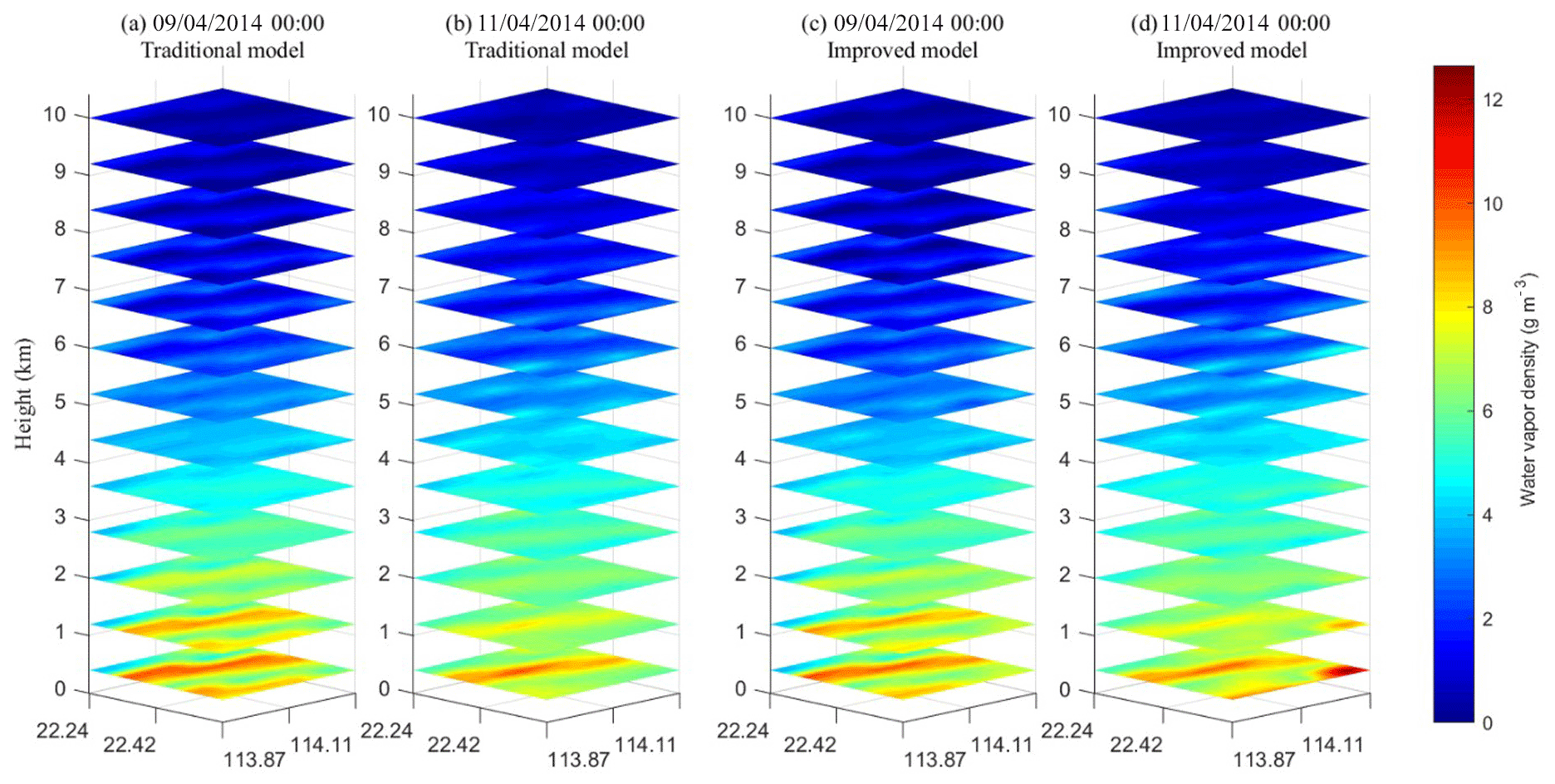
Figure 2 The layered maps of the water vapor density from (a, b) the traditional model and (c, d) the improved model at specific epochs, (a, c) 00:00 UTC on 9 April 2014 and (b, d) 00:00 UTC on 11 April 2014.

4.2 The accuracy information of the everyday distribution scenario

To prove whether the accuracy of the improved model is better than that of the traditional model on the everyday time scale, the RMSE improvement percentage is obtained from all ECMWF comparative points (a total of 12) at two epochs each day using both the layered optimal polynomial functions and the traditional method. Figure 3 shows that the percentage of RMSE improvement per day is mostly positive, and the percentage of 11 April can even approach 12 %, indicating that the improvement seems to be appreciable. This improvement shows that the accuracy of the improved model is mostly superior to that of the traditional model in everyday distribution; however, on 7, 9, and 15 April, the RMSE improvement percentage is negative. This might be due to the heavy showers bringing rapid water vapor changes from 7 to 8 April and on 14 April, which is difficult for fitting the polynomial function well with the unstable water vapor. However, since negative percentages do not exceed −1 %, the accuracy of the improved model could be considered basically equivalent to that of the traditional model for these 4 days.

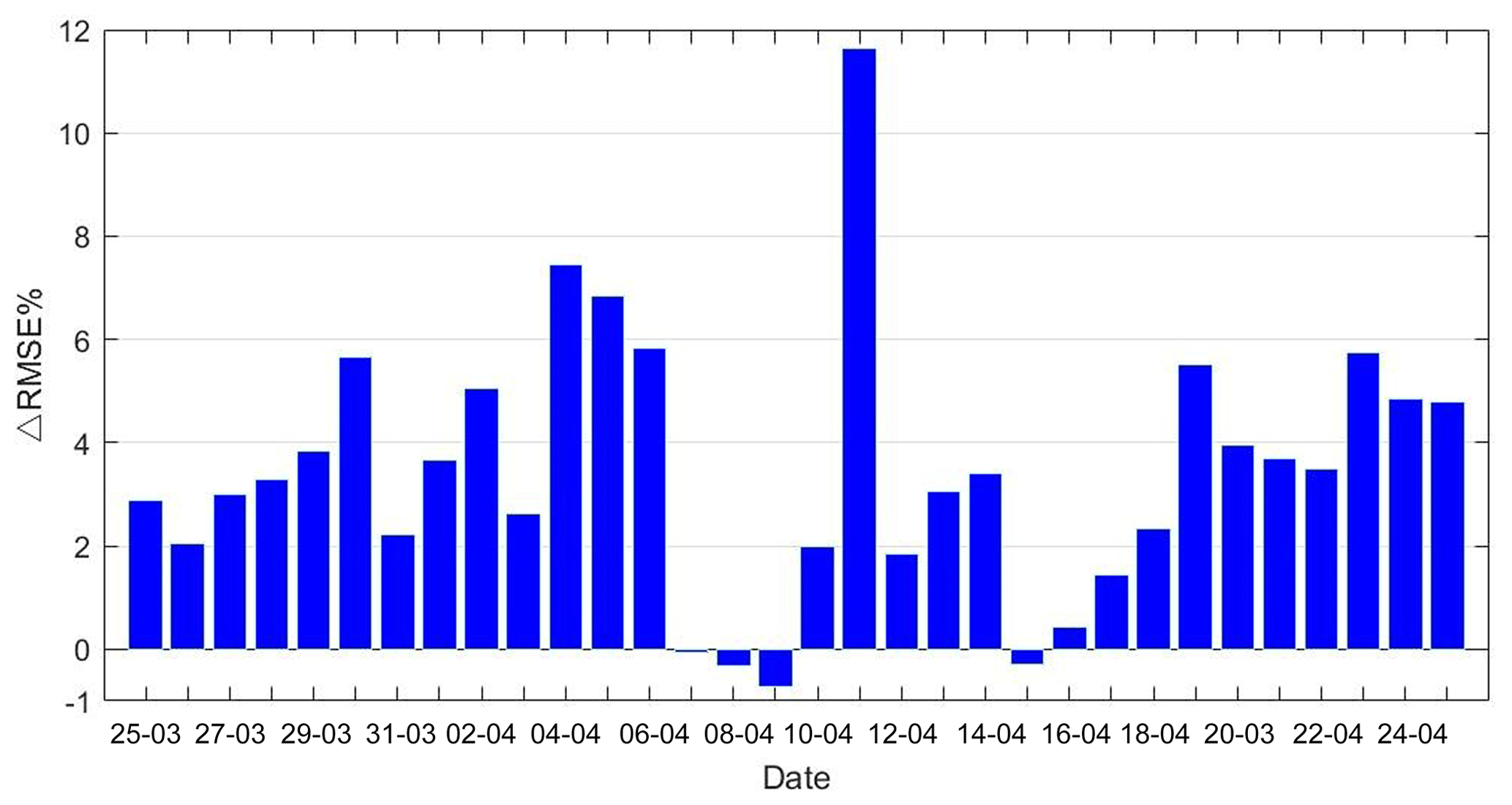
Figure 3 Everyday distribution statistics of daily RMSE improvement percentage between 25 March and 25 April 2014.

In addition, the overall RMSE and bias of the residuals are obtained from the ECMWF comparative points (a total of 12) in two epochs under the entire everyday distribution scenario. The statistical results are shown in Table 3 below.

Table 3 Statistics of two models' tomography accuracy with respect to ECMWF data in the everyday distribution scenario for the experimental period (unit: g m⁻³).

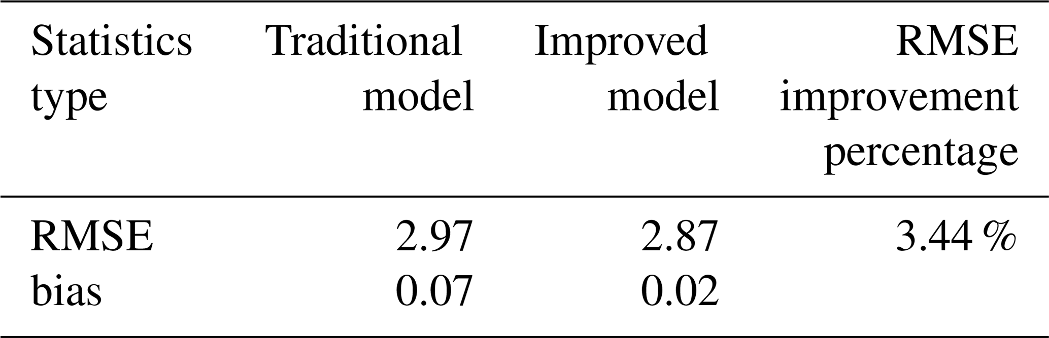
Table 3 shows that the RMSE obtained by the improved model is 3.44 % smaller compared to that of the traditional one. The bias of the improved model is more close to zero, indicating that the improved model has better stability and less systematic deviation from the comparative data. The better accuracy shows the superiority of the improved model.

4.3 The accuracy information of rainy and non-rainy scenarios

To further analyze the reliability of the improved model compared with the traditional model in different weather conditions, according to the distribution of rainy days in Table 1, all the rainy days data and non-rainy days data are used separately for tomography to obtain the RMSE and bias of the residuals under corresponding weather conditions. The number of matching points is still 12 (see Fig. 1). The overall statistical results are shown in Table 4.

Table 4 Statistics of two models' tomography accuracy with respect to ECMWF data in the rainy scenario and the non-rainy scenario for the experimental period (unit: g m⁻³).

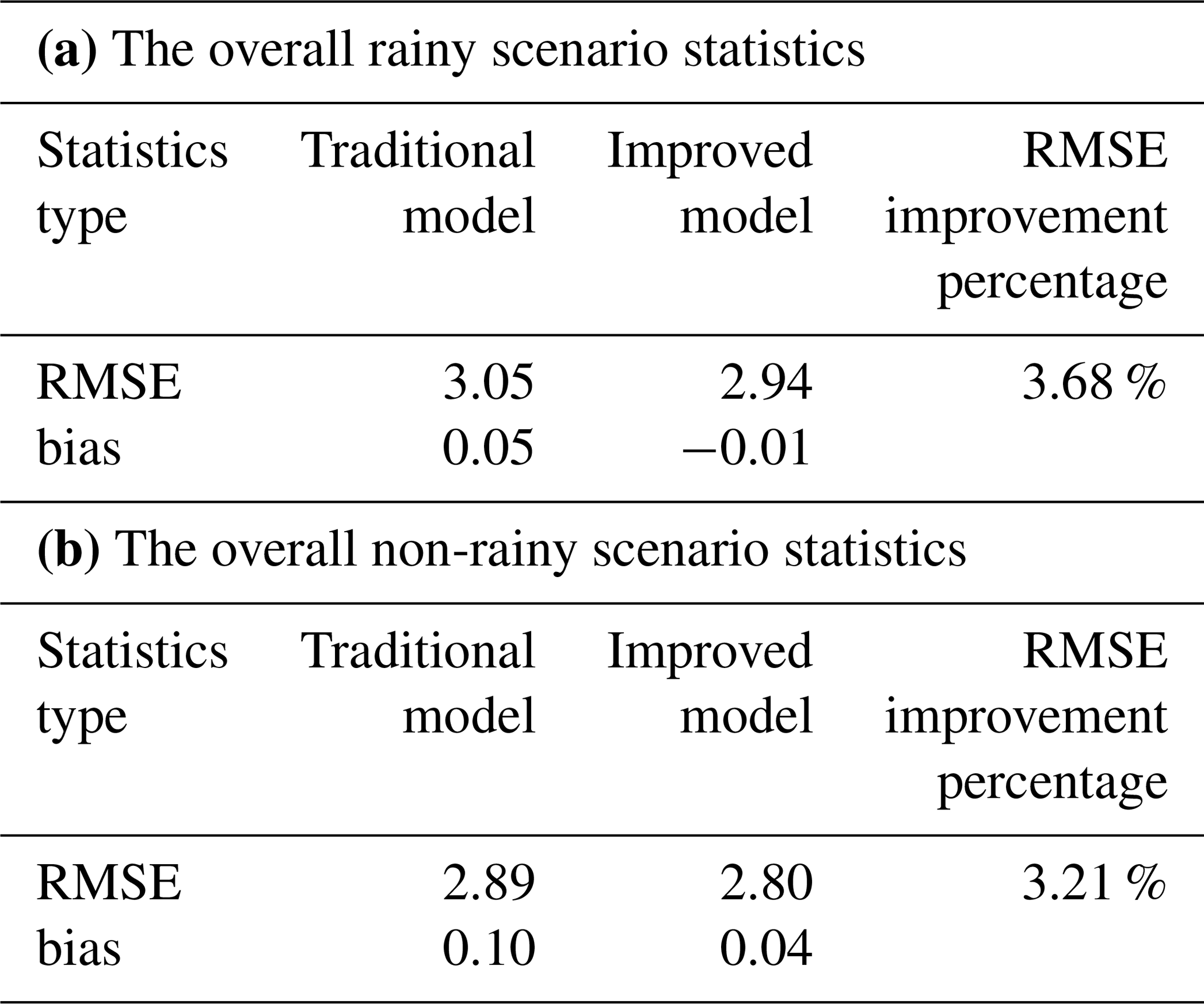
Table 4a shows that the RMSE and bias of the residuals calculated by the improved model are better than those of the traditional model using data from rainy days. The RMSE of the improved model is 3.68 % better than that of the traditional model, indicating that the accuracy of the new model is superior. The improved model bias is more close to zero than that of the traditional one, which means the improved model has an increase in stability and a reduction in the system error. Using data from non-rainy days, the RMSE and bias of the residuals calculated by the improved model are also better than those of the traditional model (see Table 4b). The RMSE improvement percentage is 3.21 %, also indicating the improved model has enhanced accuracy. Besides, the improved model bias is more close to zero, making the system error weak. Table 4 also shows that the RMSE improvement percentage of the rainy days is better than that of the non-rainy days. This finding shows that the improved model is more suitable for obtaining the tomographic results when heavy water vapor changes occur.

4.4 The accuracy information of voxels with and without GNSS-ray penetration scenarios

In the traditional pixel-based water vapor tomography model, the water vapor density in the voxels without GNSS rays passing through depends on the accuracy of the water vapor density in the adjacent voxels with GNSS-ray penetration. However, the improved model uses the layered optimal polynomial functions for overall fitting to obtain the water vapor density in voxels without penetrating GNSS rays. To determine if the layered optimal polynomial function of the improved model contributes better to the accuracy of the water vapor density, the scenarios of voxels with and without GNSS-ray penetration, as described in Sect. 3.2, were designed. After obtaining the RMSE and bias of the residuals using the improved and traditional tomography models separately under designed scenarios, the overall accuracy information of voxels with and without GNSS-ray penetration is shown in Table 5.

Table 5 Statistics of two models' tomography accuracy with respect to ECMWF data in the voxels with and without penetrating GNSS rays for the experimental period (unit: g m⁻³).

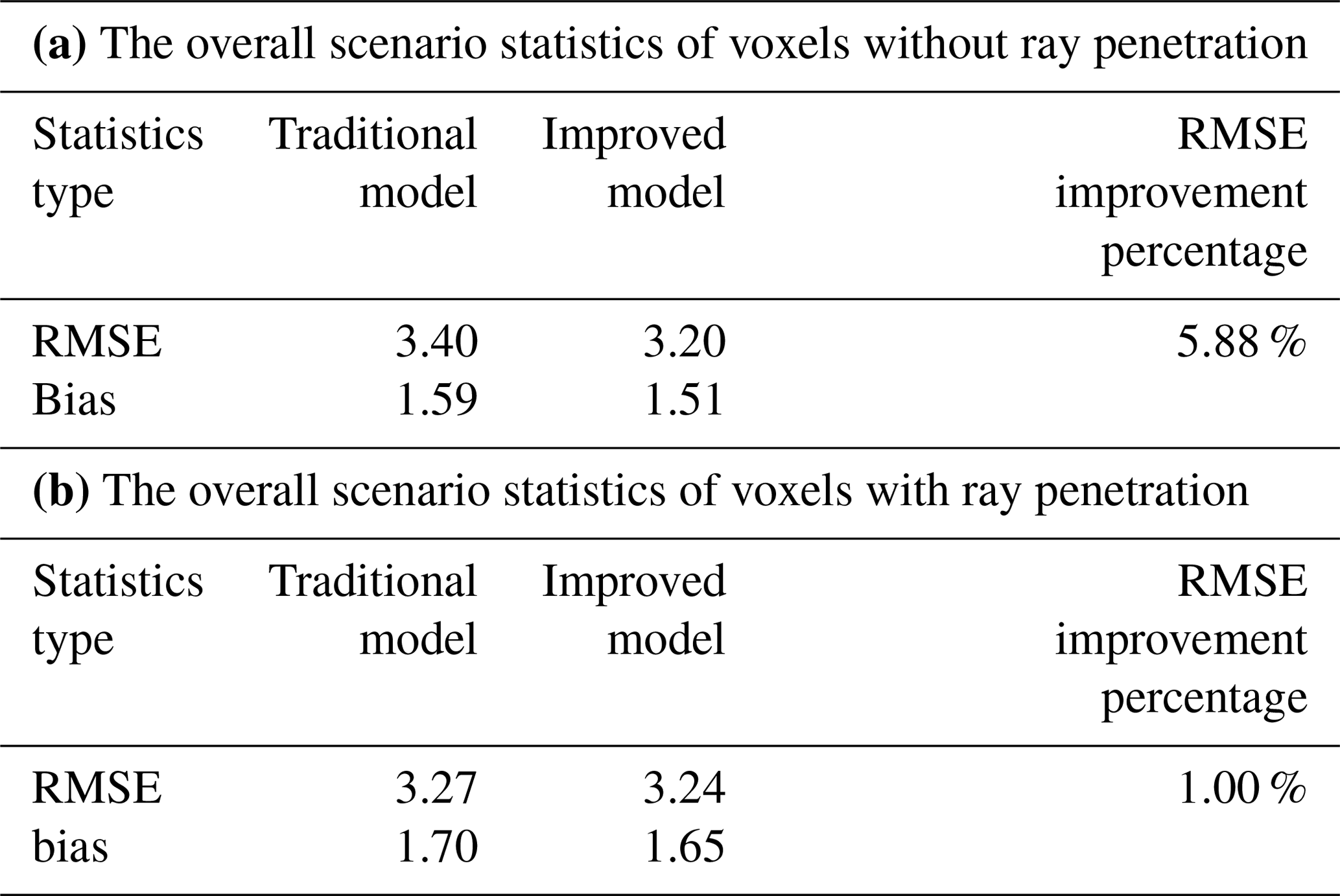
Table 5a shows that the RMSE and bias of the residuals calculated by the improved model are better than those of the traditional model in the scenario of voxels without GNSS-ray penetration. Moreover the RMSE of improved tomography model is 5.88 % better than that of the traditional model, and the bias decreased from 1.59 to 1.51 g m⁻³. To a certain extent, results show that the improved model is more advantageous for obtaining the water vapor density from the voxels without GNSS-ray penetration, which is consistent with the initial hypothesis: the traditional model uses empirical constraint equations in Sect. 2.1.2, Eq. (7), which are unable to represent the actual distribution of the water vapor density from voxels without GNSS-ray penetration well. However, the improved model uses the relatively accurate water vapor density from voxels with GNSS-ray penetration as the observation values to further fit the water vapor density in voxels without GNSS-ray penetration. Therefore, the improved model can better reflect the actual layered situation of continuous water vapor changes, and the accuracy is naturally better. In addition, in the scenario of voxels with GNSS-ray penetration, the RMSE and bias obtained by the improved model are also superior to those of the traditional models (see Table 5b). The RMSE calculated by the improved model is 1 % higher than that of the traditional model, and the bias reduced from 1.7 to 1.65 g m⁻³, which could prove the reliability of the improved model.

In order to double-check if the improved model in the scenario of voxels without GNSS-ray penetration shows a better result in the vertical water vapor distribution, the water vapor density profiles for different altitudes at specific times are given in Fig. 4. Two times (00:00 UTC on 11 April 2014 and 12:00 UTC on 11 April 2014) are chosen, since they correspond to the maximum percentage of RMSE improvement during the experiment period of 32 days. Figure 4 shows that in the scenario of voxels without GNSS-ray penetration, the water vapor profile of the improved model matches that of ECMWF data better than the traditional model, especially in the bottom layers, which again implies that the water vapor density derived from the improved model is superior to that of the traditional one in the scenario of voxels without GNSS-ray penetration.

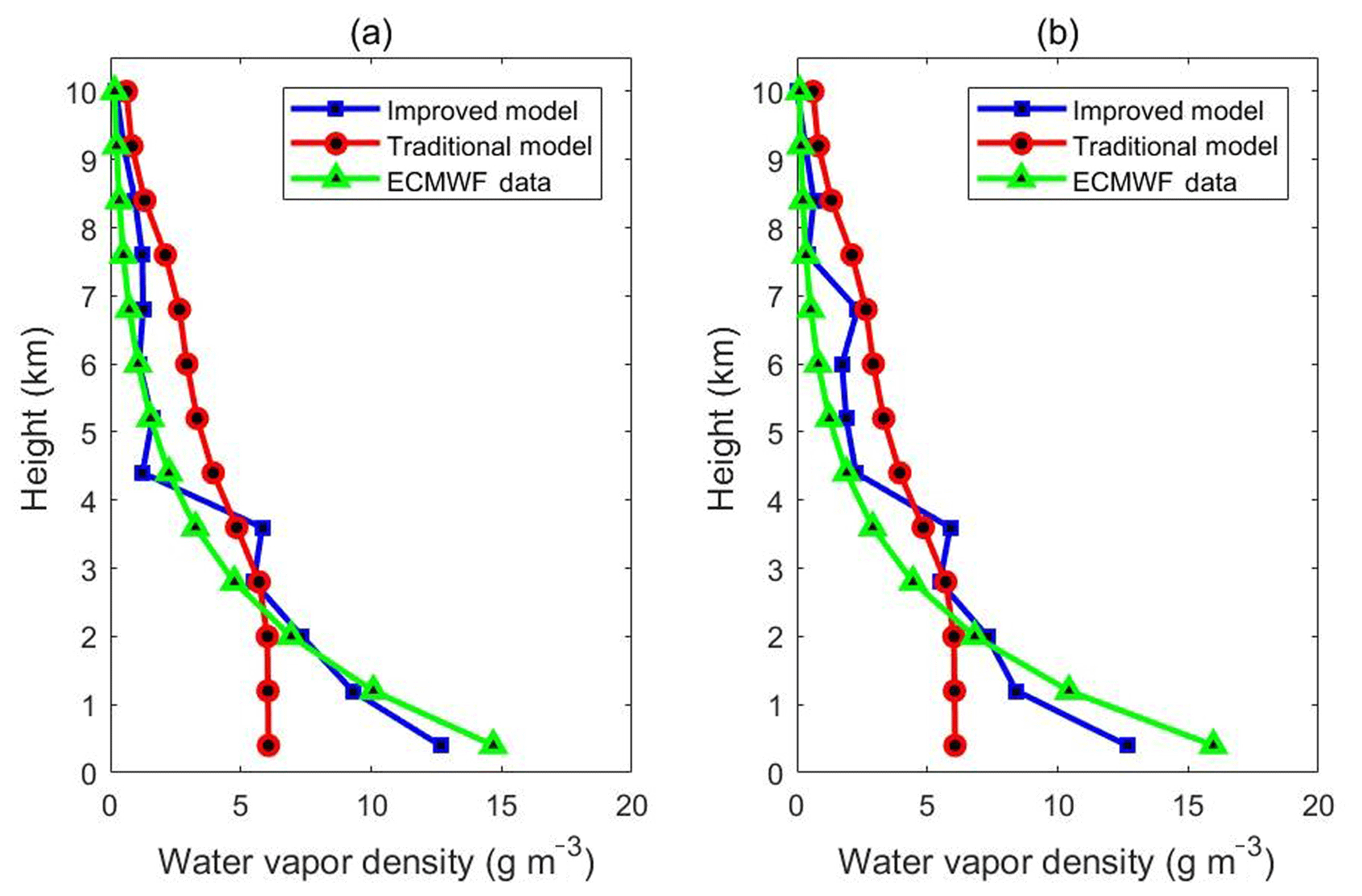
Figure 4 Water vapor profiles derived from ECMWF and two models in the scenario of voxels without penetrating GNSS rays, (a) and (b) are periods of 00:00 UTC on 11 April 2014 and 12:00 UTC on 11 April 2014, respectively.

Furthermore, to directly compare the vertical accuracy of the water vapor density derived from different altitudes in the scenario of voxels without penetrating GNSS rays, the tomographic results (25 March to 25 April 2014) from two different tomography models are analyzed. Figure 5 shows the percentage of RMSE improvement and the relative error of the water vapor density changing with altitude. The percentage of RMSE improvement in Fig. 5 is defined as the same as Eq. (16), and the relative error is defined by using Eq. (17):

$$\begin{array}{}\text{(17)}& \mathrm{RE}={\displaystyle \frac{\mathit{\rho }-{\mathit{\rho }}_{\mathrm{ECMWF}}}{{\mathit{\rho }}_{\mathrm{ECMWF}}}},\end{array}$$

where RE is the relative error, ρ represents the water vapor density derived from the traditional or improved tomography model, and ρ_ECMWF is the water vapor density derived from ECMWF grid data.

It can be observed in Fig. 5 that in the scenario of voxels without GNSS-ray penetration the percentage of RMSE improvement is positive in lower layers while negative in some middle and upper layers, which could prove that the improved model enhances the accuracy of tomography results in most layers when there are few voxels with GNSS-ray penetration, especially in the bottom layers. Due to the lack of GNSS observation data, the accuracy in the bottom layer of tomographic results is generally low. In addition, Fig. 5 shows in the scenario of voxels without GNSS-ray penetration, and the relative error begins to decrease with the altitude and then increases above 3 km. When the altitude is higher, the relative error becomes larger because of the small water vapor values in the upper layers, and a very tiny difference could cause a large relative error between the models and the ECMWF data.

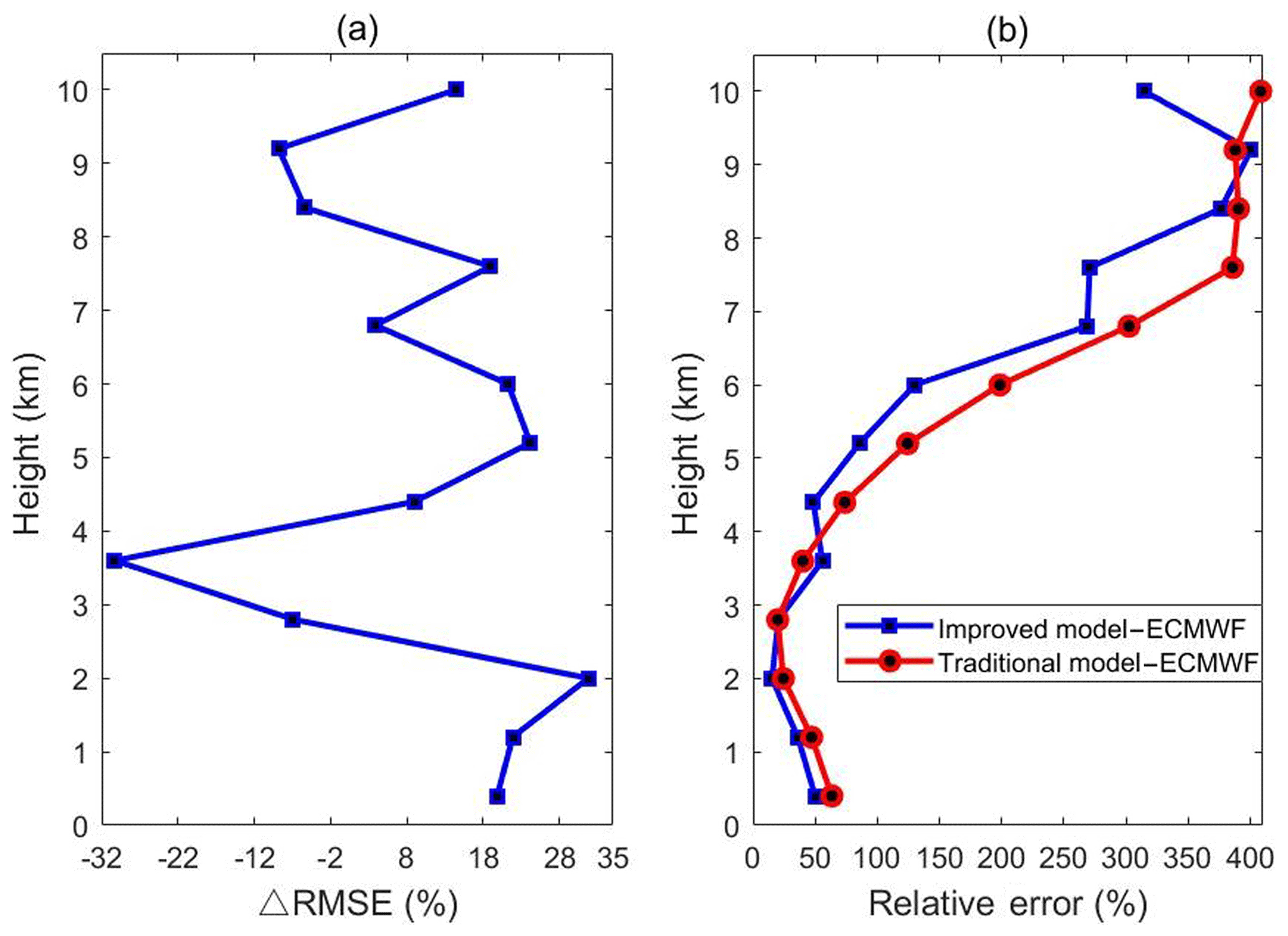
Figure 5 In the scenario of voxels without GNSS-ray penetration (a) the percentage of RMSE improvement and (b) the relative error change with height (the blue curve and red curve are derived from the differences between the profiles of the improved model, the traditional model and ECMWF grid data, respectively, for 64 epochs from 25 March to 25 April 2014).

5 Water vapor comparison with radiosonde data

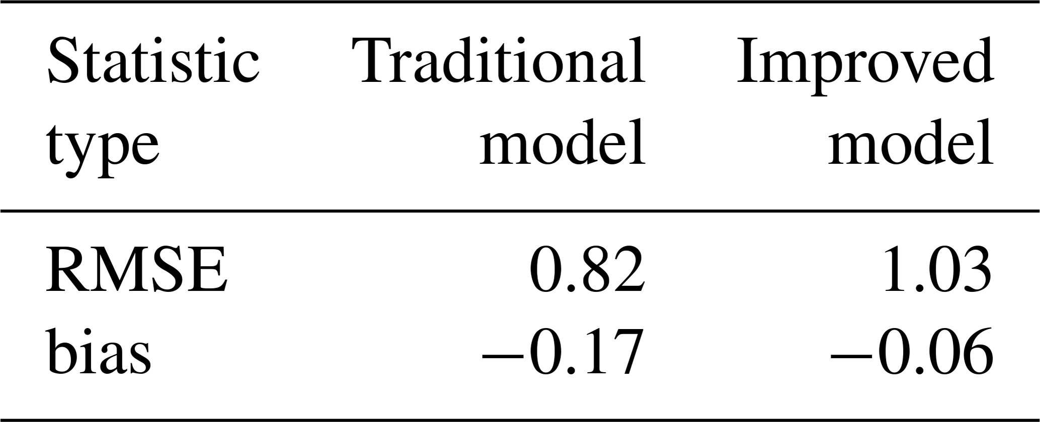
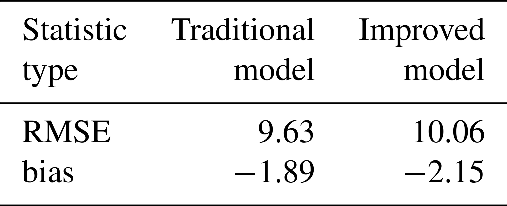
As radiosonde data can provide fairly accurate vertical profiles of tropospheric water vapor (Niell et al., 2001), in this paper, the water vapor profiles derived from radiosonde data, as a reference, are used to validate the tomographic results from two models to show if the improved model would be more efficient than the traditional one. In Hong Kong, there is one radiosonde station located at King's Park (shown in Fig. 1) where radiosonde balloons are launched twice daily, at 00:00 and 12:00 UTC, respectively. Water vapor profiles derived from the improved model and the traditional model for the location of the radiosonde station are compared with that derived from radiosonde data at 00:00 and 12:00 UTC daily for the experimental period of 32 days. The overall statistical results are shown in Table 6. The RMSE and the bias of the improved model are 1.03 and −0.06 g m⁻³, respectively, and the values of the traditional model are 0.82 and −0.17 g m⁻³, respectively, which indicates that the RMSE of the improved model is not as good as the traditional model, while the bias of the improved model is a little better than that of the traditional one. The reason for poor accuracy of the improved model could be systematic differences between the training source ECMWF data and the radiosonde data. Besides, as shown in Fig. 1, the location of the radiosonde station is close to one GNSS station (HKSC), leading to the voxels for the location of the radiosonde station having GNSS-ray penetration. Since the improved model has the advantage of only obtaining water vapor density from voxels without GNSS-ray penetration, this situation cannot show the superiority of the improved model.

Table 6 Statistics of two models' tomography accuracy with respect to radiosonde data for the experimental period (unit: g m⁻³).

In addition, water vapor profiles obtained by two models and radiosonde data are compared for the specific two epochs, at 00:00 UTC on 25 March and 00:00 UTC on 7 April 2014, shown in Fig. 6. Those two times are selected because they correspond to the non-rainy day and heavy rainfall day, which could be more comprehensive and representative for the comparison results of water vapor profiles. It can be seen from Fig. 6 that two models in the non-rainy day match the radiosonde data a little better than those in the rainy day. The traditional model shows better comparison results in upper layers than those of the improved model, while the two models have almost the same comparison results in the middle and lower layers. The reason for poor performance in the lower layers might due to abundant water vapor in the bottom troposphere as well as the division of the vertical resolution. Compared to the radiosonde data, with almost the same accuracy and profile matching results as the traditional model, the improved model still has the advantage of the convenient and efficient expression.

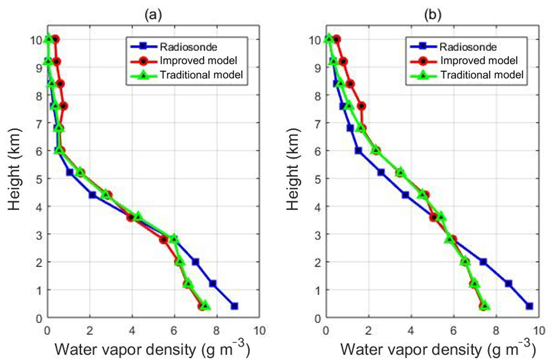
Figure 6 Water vapor profile comparison derived from different tomographic methods and radiosonde, (a) a non-rainy day at 00:00 UTC on 25 March 2014, and (b) a rainy day at 00:00 UTC on 7 April 2014.

6 SWV comparison

In order to further verify the reliability of the improved model, 5 days are randomly selected from different weather conditions to make assessments on the reconstructed SWVs of two models (see Table 7). The comparison between measured SWVs and the ones derived from tomography results of two models is performed, and the average RMSE and bias are shown in Table 8. The RMSE and bias of SWVs obtained from tomography results of two models are almost the same under different weather conditions, which indicates that the reconstructed SWVs of the improved model have similar accuracy to that of the traditional one. Since the improved model has the advantage of expressing the water vapor distribution more expediently, the similar accuracy of two models in SWV comparison shows the reliability and superiority of the improved model.

Table 7 Statistics of two models' accuracy of SWVs for different weather conditions for 5 days (unit: mm).

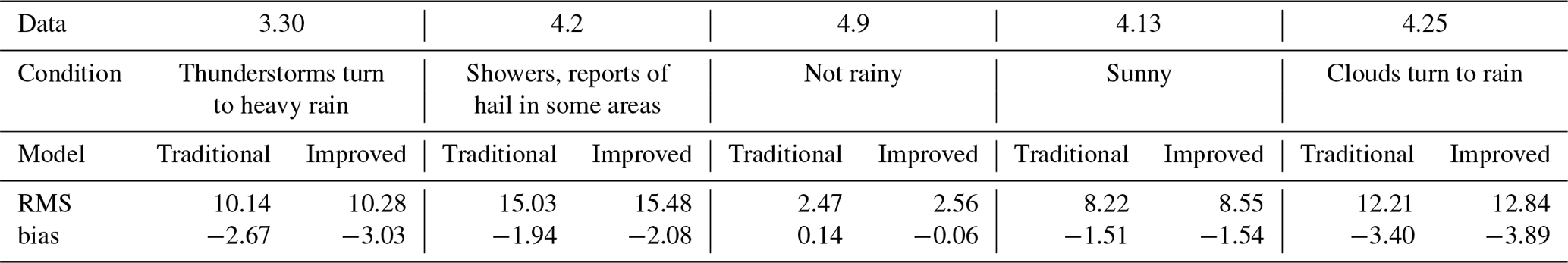
Table 8 Statistics of two models' average accuracy of SWVs for the experimental period (unit: mm).

7 Conclusions

In this paper, an improved pixel-based water vapor tomography model has been proposed that is much more concise and convenient in expression than the traditional one. Using only the layered optimal polynomial coefficients, the three-dimensional water vapor distribution in the tomography region could be described. By using the SatRef GNSS network observation data in Hong Kong between 25 March and 25 April 2014, the RMSE and bias have been assessed in six scenarios. The scenarios include the spatial distribution scenario and the everyday distribution scenario, the rainy scenario and the non-rainy scenario, and the voxels with and without GNSS-ray penetration scenarios. The results demonstrate that in either case, the RMSE and bias of the improved model are better than those of the traditional model. Among these scenarios, when there are voxels without GNSS-ray penetration, the RMSE improvement percentage can be significantly increased up to 5.88 %, which shows that the improved model is more advantageous for obtaining the water vapor density from voxels without GNSS-ray penetration. Using radiosonde data for evaluation, it is proven that, with almost similar accuracies, the improved model is more efficient in expression than the traditional one. However, some shortcomings still remain in the improved model. For example, more or less, the water vapor accuracy of the improved model is still affected by the traditional model, and the layered optimal polynomial functions are limited by the size of the tomographic area and the situation of dividing voxels. In the future, the function-based water vapor tomography model, which is free from the above limitations, should be studied. It is expected that the function-based water vapor tomography model will be more conveniently used when the expression parameters of the function part could be obtained directly from SWVs.