Effect of latitudinally displaced gravity wave forcing in the lower stratosphere on the polar vortex stability

In order to investigate the impact of a locally confined gravity wave (GW) hotspot, a sensitivity study based on simulations of the middle atmosphere circulation during northern winter was performed with a nonlinear, mechanistic, general circulation model. To this end, we selected a fixed longitude range in the East Asian region (120–170^∘ E) and a latitude range from 22.5 to 52.5^∘ N between 18 and 30 km for the hotspot region, which was then shifted northward in steps of 5^∘. For the southernmost hotspots, we observe a decreased stationary planetary wave (SPW) with wave number 1 (SPW 1) activity in the upper stratosphere and lower mesosphere, i.e., fewer SPWs 1 are propagating upwards. These GW hotspots lead to a negative refractive index, inhibiting SPW propagation at midlatitudes. The decreased SPW 1 activity is connected to an increased zonal mean zonal wind at lower latitudes. This, in turn, decreases the meridional potential vorticity gradient (q_y) from midlatitudes towards the polar region. A reversed q_y indicates local baroclinic instability, which generates SPWs with wave number 1 in the polar region, where we observe a strong positive Eliassen–Palm (EP) divergence. As a result, the EP flux increases towards the polar stratosphere (corresponding to enhanced SPW 1 amplitudes), where the SPWs with wave number 1 break, and the zonal mean zonal wind decreases. Thus, the local GW forcing leads to a displacement of the polar vortex towards lower latitudes. The effect of the local baroclinic instability indicated by the reversed q_y also produces SPWs with wave number 1 in the lower mesosphere. The effect on the dynamics in the middle atmosphere due to GW hotspots that are located northward of 50^∘ N is negligible, as the refractive index of the atmosphere is strongly negative in the polar region. Thus, any changes in the SPW activity due to the local GW forcing are quite ineffective.

1 Introduction

During winter, the dynamics of the middle atmosphere are mainly dominated by the polar vortex. The polar vortex develops due to the lack of incoming solar radiation and is modified by the impact of atmospheric waves with different spatial and temporal scales (Douville, 2009). The most important characteristic of atmospheric waves is their ability to transport and deposit energy and momentum. In particular, gravity waves (GWs), which mainly develop in the troposphere, distribute energy and momentum throughout the whole atmosphere; thus, GWs maintain the circulation and the thermal structure of the upper atmosphere (Fritts and Alexander, 2003). They also contribute to turbulence and mixing between all vertical layers. Their most important sources are orography (Smith, 1985; Nastrom and Fritts, 1992), convection (Tsuda et al., 1994), jet sources (Plougonven and Zhang, 2014) or spontaneous adjustment processes (Fritts and Alexander, 2003). Strongly depending on the phase speed c and the background wind u, GWs are able to propagate into the middle atmosphere. Due to the exponentially decreasing density of the atmosphere, the GW amplitude exponentially increases with height if the GWs propagate conservatively under background conditions that are constant with height. Usually, the GW spectrum is already saturated in the stratosphere, which means that GW amplitudes cannot grow anymore and, according to the linear theory, partly break. This effect becomes stronger as their phase speed c gets closer to the background wind u. If c is equal to u, the GW encounters its critical line and cannot propagate anymore (Lindzen, 1981). Thus, GWs propagating in the opposite direction of the background wind are usually observed in the middle atmosphere. Moreover, GWs that are faster than the background wind are able to propagate, but they are mostly filtered out by the strong polar-night jet when c becomes equal to u (at the latest). In the mesosphere GWs, which are propagating in the opposite direction of u, saturate and deposit their momentum. For this reason, the wind reverses in the upper mesosphere and lower thermosphere (MLT) (Lindzen, 1981; Holton, 1982). The transfer of energy and momentum by breaking GWs is also called “GW drag”.

Owing to the variety of their sources, GWs have a large spatial and temporal variability. To capture the global distribution of GWs, the potential energy (E_pot), momentum flux (MF) or stability indicators (Pišoft et al., 2018) can be estimated using satellite data (Ern et al., 2004; Fröhlich et al., 2007; Hoffmann et al., 2013; Schmidt et al., 2016). These numerous observational studies highlight a number of different local GW hotspots, which are mainly generated by orography and convection. The most common GW hotspots are the orographically induced GW hotspots near the Alps (Hierro et al., 2018), the Andes (Llamedo et al., 2009; Alexander et al., 2010; Lilienthal et al., 2017), the Antarctic Peninsula (Moffat-Griffin et al., 2010), the Himalayas (Kumar et al., 2012), the Mongolian Plateau (White et al., 2018), the Rocky Mountains (Lilly et al., 1982) and in the Scandinavian region (Kirkwood et al., 2010). Typically, satellite observations show a characteristic structure of enhanced GW activity in the subtropical stratosphere that is caused by deep convection over Southeast Asia, America, Africa or the Maritime Continent in the respective summer season (Jiang et al., 2004; Wright and Gille, 2011; Ern and Preusse, 2012). Reliable estimates of GW drag from observations are generally difficult. Several methods have been established to derive the GW drag from satellite (e.g., Ern et al., 2014, 2016) or radar measurements (e.g., Reid and Vincent, 1987); however, the uncertainties of these estimates are quite large.

Model studies have indicated that GWs can already break in the lower stratosphere (LS) (e.g., Plougonven et al., 2008; Constantino et al., 2015), which leads to an additional transfer of momentum and energy in this region. In connection with high planetary wave (PW) activity, this greatly affects the stability of the polar vortex and can cause a sudden stratospheric warming (SSW) (Albers and Birner, 2014). This effect has also been observed in satellite measurements that have shown enhanced GW drag before SSWs (Ern et al., 2016). Thus, an additional GW forcing may lead to a preconditioning of the polar vortex.

This study focuses on the role of the zonal position of localized GW breaking areas and their effects on the middle atmosphere dynamics. It is motivated by the findings of Šácha et al. (2015), who focused on the East Asian and North Pacific (EA/NP) region near Japan, where they observed a GW hotspot that was active during equinoxes and winter solstices. The GWs are orographically and convectively generated due to the topography located directly at the coastline and the warm Kuroshio Current. Šácha et al. (2015) analyzed the local instabilities by calculating the Richardson number and by analyzing reanalysis data and found that the GWs break in this area. Based on these results, they simulated the observed Asian GW breaking hotspot with a general circulation model (GCM) and analyzed its effect on the middle atmosphere circulation (Šácha et al., 2016). According to previous publications, e.g., by Smith (2003), Lieberman et al. (2013) or Matthias and Ern (2018), Šácha et al. (2016) observed a forcing of additional stationary planetary waves (SPWs) due to a longitudinally variable GW drag. We pursue this idea by shifting the EA/NP hotspot meridionally while keeping its longitude range fixed to obtain information about its impact on the middle atmosphere at different latitudinal positions. Therefore, the EA/NP GW hotspot is our starting point, from which we displace the GW hotspot towards lower and higher latitudes in 5^∘ steps. In Sect. 2 of this paper, we provide a brief description of the GCM and detail the implementation of the GW hotspot within the GCM. In Sect. 3 we describe and discuss the observed effects of the GW hotspots on the circulation of the middle atmosphere by analyzing the SPW activity and the propagation conditions. Finally, the conclusions and outlook are presented in Sect. 4.

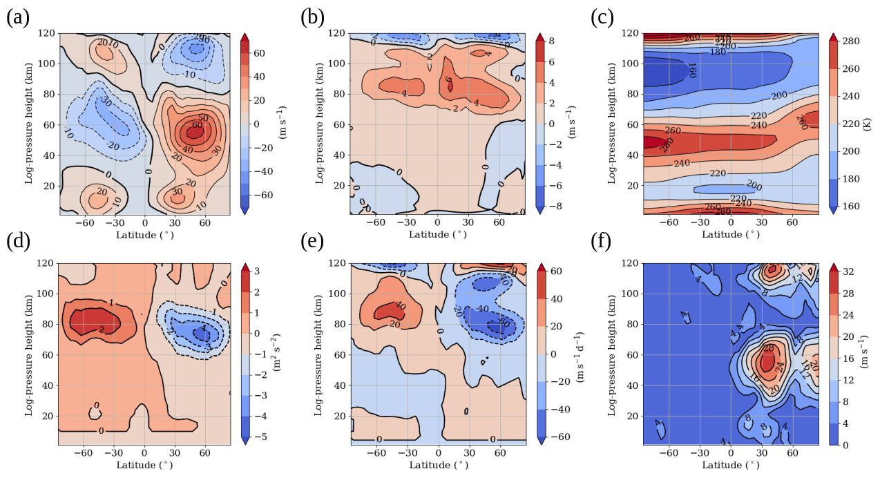
Figure 1 January zonal and monthly mean of the (a) zonal wind (m s⁻¹), (b) meridional wind (m s⁻¹), (c) temperature (K), (d) zonal GW fluxes (m² s⁻²), (e) zonal wind acceleration due to breaking GWs (m s⁻¹ d⁻¹) and (f) SPW 1 amplitude (m s⁻¹) extracted from the zonal wind of the reference simulation.

2 Numerical model experiments

2.1 Model description and setup

To investigate the effect of localized GW breaking hotspots in the LS, simulations were performed using the Middle and Upper Atmosphere Model (MUAM, Pogoreltsev et al., 2007). MUAM is a nonlinear mechanistic 3-D grid point model, which is an updated version of the COMMA-LIM general circulation model (Fröhlich et al., 2003a, 2007; Jacobi et al., 2006). The model extends in 56 layers up to an altitude of about 160 km in logarithmic pressure height $z=-H\ln (p/p_{\mathrm{0}})$ with a constant scale height of H=7 km and a reference pressure of p₀=1000 hPa. Depending on the temperature profile, the logarithmic pressure height used can differ from the geometric height. However, at altitudes below 80 km, this difference is negligibly small. At 110 km the deviation increases up to 5 km, whereas the highest logarithmic pressure level of about 160 km may correspond to a geometrical height between 300 and 400 km. In the lowermost 10 km, zonal mean temperatures are nudged to the 2000–2010 mean monthly mean ERA-Interim (Dee et al., 2011) zonal mean temperatures to correct the climatology of the troposphere, which is not included in the model in detail (Jacobi et al., 2015; Lilienthal et al., 2018). Furthermore, at 1000 hPa, which defines the lower boundary of the model, SPWs with wave numbers 1, 2 and 3 are forced, which are extracted from the 2000–2010 mean ERA-Interim monthly temperature and geopotential reanalysis data. The horizontal resolution of the model is 5^∘ in latitude and 5.625^∘ in longitude and the vertical resolution is 2.842 km. The model solves the primitive equations in flux form (e.g., Jakobs et al., 1986). MUAM includes parameterizations to simulate subgrid processes such as GWs, absorption of solar radiation or infrared cooling. The absorption of radiation is realized according to Strobel (1986). This parameterization is focused on the absorption processes due to trace gases such as H₂O (absorber in the troposphere) as well as CO₂ and O₃ (absorbers in the stratosphere). Water vapor and ozone fields are prescribed. The heating rates are calculated by absorption bands representing the wavelength interval at which these trace gases absorb the atmospheric radiation. The infrared emission of CO₂ is parameterized following Fomichev et al. (1998), and ozone infrared cooling in the 9.6 µm band is calculated following Fomichev and Shved (1985).

GWs are parameterized after an updated linear scheme (Lindzen, 1981; Jakobs et al., 1986) with multiple breaking levels (Fröhlich et al., 2003b; Jacobi et al., 2006). GW amplitudes are included at an altitude of 10 km as a zonal mean with a global average of 1 cm s⁻¹ for the vertical velocity perturbation. This value is weighted by a prescribed zonal mean GW amplitude distribution based on E_pot data obtained from GPS radio occultation measurements (Šácha et al., 2015; Lilienthal et al., 2017). Although the E_pot data still contain Kelvin waves and other possible wave structures with short vertical wavelengths, which may introduce biases, the GW amplitude distribution is more realistic than the hyperbolic tangent function of the latitude, which was used in earlier experiments (Jacobi et al., 2006), and leads to an improvement of the zonal mean GW climatology. It shows maximum GW amplitudes (not shown here) at the Equator (convectively generated GWs) and at midlatitudes (orographically induced GWs). At each grid point 48 waves are induced that propagate in eight different directions with six different phase speeds ranging from 5 to 30 m s⁻¹.

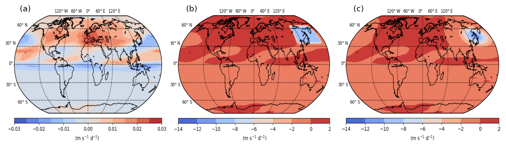
Figure 2 Zonal GW drag (m s⁻¹ d⁻¹) at 26.9 km for the reference (a) and the H3 hotspot simulation as a box (b) and as a Gaussian distribution (c) for the last 30 d of analysis. Note the different scale for panel (a).

In this configuration, based on January decadal mean (2000–2010) ERA-Interim reanalysis data, we create a reference simulation with a spin-up period of 270 d (days), in which the mean circulation is built up and different waves such as PWs and tides are generated. The declination and the ozone and carbon dioxide concentration are fixed to avoid further non-zonal structures being induced in addition to the enhanced GW forcing. The declination corresponds to 15 January (referring to the middle of the month), and the ozone and carbon dioxide data are taken from the year 2005 (referring to the middle of the decade). For the analysis, a time interval of 120 d with a temporal resolution of 2 h after the spin-up period was modeled. Šácha et al. (2016) have already analyzed the effect of the Asian hotspot with MUAM by performing a sensitivity study with regard to the strength of the GW forcing in the stratosphere. Their analysis time period was much shorter and the declination of the sun was different. They also nudged the model zonal mean temperature up to 30 km. In this regard, our experimental setup might be considered superior to their simulations, especially as the nudging does not interfere with the GW forcing implemented in this new configuration. We refer to this reference simulation as “Ref”.

The state of the middle atmosphere in the Ref simulation can be seen in Fig. 1, which shows the January zonal mean zonal (Fig. 1a) and meridional wind (Fig. 1b), the temperature (Fig. 1c), zonal GW flux (Fig. 1d), the zonal wind acceleration due to breaking GWs (Fig. 1e), and the SPW 1 amplitude extracted from the zonal wind (Fig. 1f) as latitude–height plots. Each parameter is presented up to an altitude of 120 km for the winter and summer hemisphere. The zonal wind in Fig. 1a generally reproduces reference climatologies like CIRA-86 (Fleming et al., 1988) or URAP (Swinbank and Ortland, 2003), but the winter mesospheric jet is overestimated by about 10–20 m s⁻¹. The meridional circulation (Fig. 1b) extending from the summer to the winter mesopause has a maximum of 6 m s⁻¹ at about 80 km, which reproduces predictions by climatologies well (Portnyagin et al., 2004; Jacobi et al., 2009). Temperature (Fig. 1c) generally reproduces climatology values. The GW fluxes (Fig. 1d) maximize at about 80 km, with a maximum of slightly above −4 m² s⁻² in the Northern Hemisphere (NH) and 2 m² s⁻² in the Southern Hemisphere (SH). The corresponding zonal GW drag maximizes at the same altitude with about −60 m s⁻¹ d⁻¹ (40 m s⁻¹ d⁻¹) in the NH (SH) and is directed westward (eastward). The SPW 1 amplitude (Fig. 1f) extracted from the zonal wind shows maximum values at the border of the mesospheric jet maximum north of 30^∘ N between 50 and 60 km and in the polar region. This fits quite well with observations, but the amplitudes are slightly underestimated due to the overestimated mesospheric jet, filtering some of the SPWs (Xiao et al., 2009).

2.2 Experiment description

Firstly, we reproduced the experiment of Šácha et al. (2016) to check if we still obtained similar results with the slightly modified setup. To represent the Asian GW breaking hotspot in the model, we enhanced the GW drag after model day 270, i.e., after the spin-up, and ran the model for 120 d as in the Ref simulation. Hence, the zonal (GWD_u) and meridional (GWD_v) GW drag and the heating due to breaking GWs (GWD_T) were modified in the specific region of the observed GW breaking hotspot. In principle, the response to the GW drag would in turn alter the GW propagation and breaking conditions and, thus, the GW drag and its distribution. To avoid those feedback mechanisms, the GW parameterization scheme is turned off during the experiments, and the model is fed with the GW drag field from the Ref simulation. However, in the GW hotspot region, the GW drag is modified (as shown in Table 1). We intend to only analyze the steady-state impact of the local GW forcing that is not influenced by nonlinear effects.

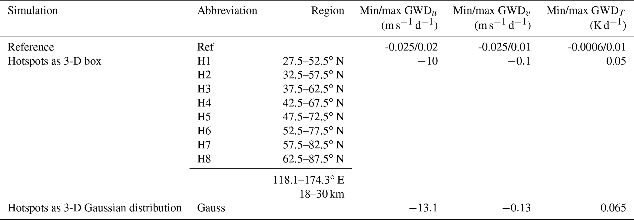
As in Šácha et al. (2016), we located the GW breaking hotspot between 37.5 and 62.5^∘ N and between 118.1 and 174.3^∘ E in an altitude range between 18 and 30 km. Note that the geographic positions refer to the model grid points; thus, at a latitudinal 5^∘ grid, the meridional size of the modeled hotspot is 30^∘. To avoid a total breakdown of the polar vortex and a fundamental change in middle atmosphere dynamics, which was already forced in the study by Šácha et al. (2016), we chose the more moderate case of −10 m s⁻¹ d⁻¹ for GWD_u, −0.1 m s⁻¹ d⁻¹ for GWD_v and a warming of 0.05 K d⁻¹ for GWD_T. We refer to this simulation as the H3 simulation, as will be described later. The distribution of the GWD_u of the Ref and the H3 simulations can be seen in Fig. 2a and b at an altitude of about 27 km for the last 30 d of analysis. We mainly concentrate on the last 30 d of analysis, as we focus on quasi-steady states and are not interested in short-term variabilities. The GWD_u of the Ref simulation varies between −0.025 and +0.02 m s⁻¹ d⁻¹ in the GW hotspot region (27.5–87.5^∘ N, 118.1–174.3^∘ E, 18–30 km). Thus, the maximum value of the H3 simulation (GWD${}_u=-\mathrm{10}$ m s⁻¹ d⁻¹ in the hotspot) is 500 times larger than the maximum westward (negative) value of the Ref simulation. The H3 mean value (mean GWD_u: −10 m s⁻¹ d⁻¹) is roughly 3300 times larger than that of the Ref simulation (mean GWD_u: 0.003 m s⁻¹ d⁻¹) within the region of the EA/NP hotspot. These maximum values of the GWD_u as well as those of the GWD_v and the GWD_T are summarized in Table 1 for the Ref and the GW hotspot simulations. In spite of the huge difference compared with the Ref simulation, the zonal GW forcing is moderate in terms of what is estimated from observations (40 m s⁻¹ d⁻¹ and more) and from GW parameterizations in this region (Šácha et al., 2018). Concerning the meridional GW drag and the heating due to breaking GWs, the maximum (mean) value of the H3 simulation is only 5 (100) times larger than that of the Ref simulation (not shown here). To investigate possible effects with regard to the position of the GW hotspot, we performed a sensitivity study. For this, we kept the longitude (118.1–174.3^∘ E) and altitude (18–30 km) range as well as the zonal extent of 25^∘ fixed, but varied the observed GW hotspot in 5^∘ steps from 27.5–52.5^∘ N (simulation H1) to 62.5–87.5^∘ N (simulation H8), while labeling the experiments in between as H2 through H7 (see Table 1).

Table 1 Overview of the mean and maximum values of the zonal and meridional GW drag and heating by GWs for the reference and hotspot simulations as a 3-D box (H1–H8) and as a Gaussian distribution (Gauss). The mean and maximum values refer to the region (118.1–174.3^∘ E, 18–30 km and the respective latitude range as listed below) of the hotspots.

To analyze the possible effects of the sharp transition zone between the unchanged and enhanced GW drag, additional simulations with a smoothed GW forcing were performed, using a 3-D Gaussian function with standard deviations of 10^∘, 22.5^∘ and 5.684 km in the zonal, meridional and vertical directions, respectively. To get the same integral forcing as in the H1–H8 simulations, the size or the intensity of the local GW forcing as a Gaussian distribution needed to be adjusted. For our experiments, we mainly increased the strength of the local GW forcing and only slightly increased the size. The maximum values for the GWD_u, GWD_v and GWD_T forcing as a 3-D Gaussian distribution were chosen to be −13 m s⁻¹ d⁻¹, −0.13 m s⁻¹ d⁻¹ and 0.065 K d⁻¹ (see Table 1), respectively. The 3-D Gaussian distribution for the H3 GW hotspot can be seen in Fig. 2c. In this paper we mainly concentrate on the 3-D GW hotspots shaped like a box when we analyze the effects on the middle atmosphere dynamics. For comparison, regarding the shape of the artificial GW forcing, we just focus on the H3 GW hotspot with Gaussian smoothed boundaries when we discuss the SPW modulation in Sect. 3.2, which may be affected by the GW hotspots with sharp boundaries.

When comparing the size of the GW hotspots it is obvious (can be seen in Fig. 5) that the area of the enhanced GW drag, which scales with the cosine of the latitude, decreases with increasing latitude. However, scaling the GW drag with latitude would lead to a much larger zonal mean GW drag at high latitudes and would result in changes in the circulation. Furthermore, the horizontal winds, which are affected by resulting nonlinear interactions, are scaled in the model equations. In the current approach, we conserve the ratio of enhanced and unchanged GW drag values within the respective latitudinal belt, which is more meaningful. Also, the horizontal wavelength of PWs becomes smaller with decreasing distance from the pole, meaning that the ratio of the width of the GW forcing and the horizontal wavelength of the PWs remains the same for the respective latitudinal belt. In the following, we will show that the spatial shape as well as the spatial size of the local GW forcing is not the most decisive factor when we compare the 3-D Gaussian distribution with the 3-D GW forcing shaped as a box. Thus, GW hotspots that are the same size may lead to comparable results.

3 Results

3.1 Hotspot effect on the background circulation

Figure 3a–h show the zonal mean zonal wind difference between each GW hotspot simulation H1–H8 and the Ref simulation (in color) as well as the zonal mean zonal wind of the Ref simulation (as contour lines) in a latitude–height plot. The position of each GW hotspot is illustrated by a red box. All experiments (H1–H8) show negative zonal wind differences with a maximum wind decrease of more than −10 m s⁻¹ in the polar region. Positive differences can be observed equatorward from an imaginary line connecting the subtropical and polar-night jet centers, with a maximum difference of 8 to 10 m s⁻¹. These zonal wind anomalies are consistent with a polar vortex that is shifted towards lower latitudes, and the wind reversal in the mesosphere is shifted upwards at lower latitudes. The strongest decrease in the zonal mean zonal wind in the polar region can be observed in the H1 simulation (Fig. 3a) and the strongest increase in zonal mean zonal wind at lower latitudes can be observed in the H3 simulation (Fig. 3c), the latter corresponds to the observed Asian GW hotspot. For GW hotspots with a southern edge north of 50^∘ N, the polar vortex is only slightly displaced towards lower latitudes. Thus, the effect of GW hotspots at higher latitudes is not as strong.

Figure 4 is arranged in the same manner as Fig. 3, but shows the temperature difference (in color) and the vertical wind difference (as contour lines). As expected, the temperature effect scales (both zonal and vertical) with the wind differences; thus, the H1–H3 simulations in Fig. 4a–c show the strongest temperature anomalies, and these once again decrease in magnitude for northward-shifted GW hotspots. Between 60 and 90^∘ N, the GW hotspot leads to a temperature increase at altitudes up to 30–35 km, but to a decrease above. The zonal mean vertical wind difference shows generally negative anomalies between 15 and 30 km at higher latitudes, which indicates a stronger downward movement connected with an adiabatic warming in the lower part of the polar stratosphere. Above 35–40 km, we observe a positive vertical wind anomaly for the H1–H3 simulations, i.e., the downward movement is reduced and leads to an adiabatic cooling anomaly. For most of the simulations, the negative anomaly in the lower part of the stratosphere is stronger than the positive anomaly above 40 km, which fits with the distribution of the temperature anomalies. In case of the H4 and H5 simulations (Fig. 4d, e), the vertical wind anomalies do not fit with the temperature anomalies. We observe an increased downward movement in a region where the temperature weakly decreases.

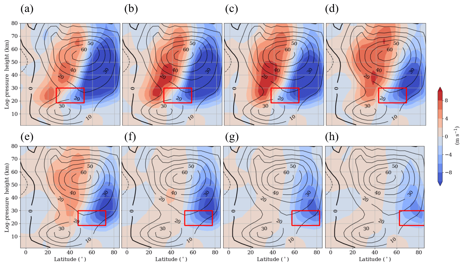
Figure 3 Zonal mean zonal wind difference between the H1–H8 simulations (a–h) and the reference simulation (H1–H8 − Ref). The colors indicate the difference between the simulations, and the contour lines show the zonal mean zonal wind of the reference simulation. Figures represent the last 30 d of the simulations. The position of each GW hotspot is represented by a red box.

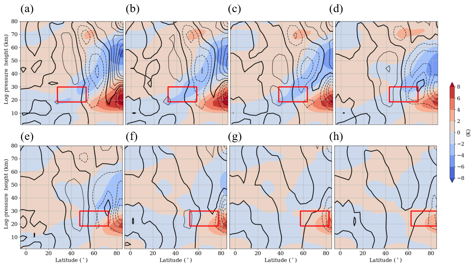
Figure 4 Zonal mean temperature and vertical wind difference between the H1–H8 simulations (a–h) and the reference simulation (H1–H8 −  Ref). The colors indicate the temperature difference between the simulations, and the contour lines show the vertical wind difference from ±0.0005 to ±0.0025 m s⁻¹ with increments of 0.0005 m s⁻¹ and a thicker zero line. Negative (positive) values are shown using dashed (solid) lines. Figures represent the last 30 d of the simulations. The position of each GW hotspot is represented by a red box.

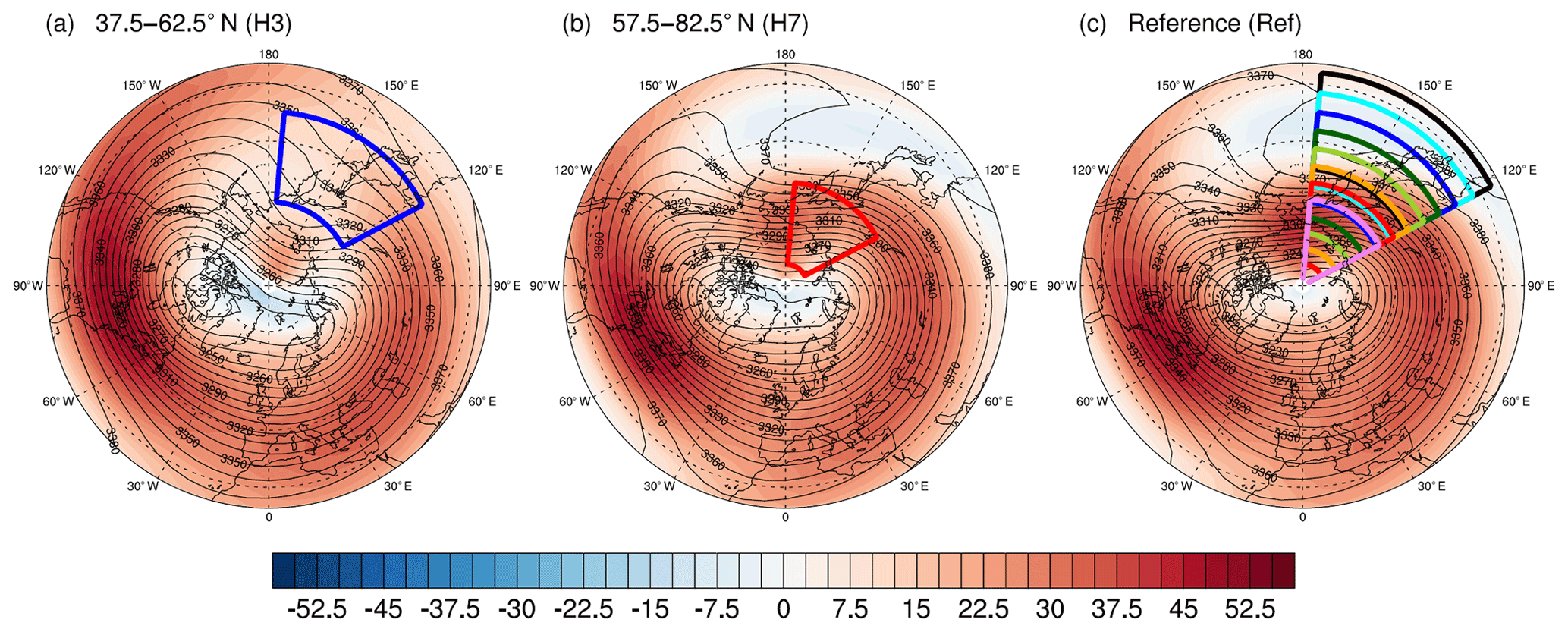
Figure 5 Zonal wind (m s⁻¹) in color and geopotential height (gpdam) as contour lines north of 25^∘ N at 35 km for the H3 (a), H7 (b) and the Ref (c) simulations, representing the last 30 d of analysis. The boxes illustrate the position of each GW hotspot: H1 (in black) to H8 (in violet). The blue (a, c) (red, b, c) box refers to the H3 (H7) simulation.

3.2 Influence on the polar vortex and anomalous SPWs

From previous publications, it is already known that a warming (cooling) of the high-latitude stratosphere (mesosphere) and related changes in the dynamics are generally connected with PW activity. This leads us to the hypothesis that the main GWD enhancement effect is due to SPW modulation, and this will be investigated in this subsection. In Fig. 5, we show the geopotential height (as contour lines) and the zonal wind (using color coding) as a polar plot at 35 km, i.e., 5 km above the region of GW forcing, for the H3 (Fig. 5a), H7 (Fig. 5b) and Ref simulations (Fig. 5c). The panels represent the last 30 d of analysis. The position of each GW hotspot is illustrated by the boxes, H1 (black) to H8 (violet), in Fig. 5c. The polar vortex of the Ref simulation is stable (not displaced or split) and located near the North Pole (Fig. 5c). Between 30 and 55^∘ N, the zonal wind of the Ref simulation is easterly in one part of the EA/NP region due to the Aleutian High (AH). This means that the GW forcing, which normally acts against the westerly zonal mean zonal wind, locally strengthens the zonal wind. Between 55 and 90^∘ N there is a strong westerly wind between East Asia and Alaska; thus, the GW forcing there acts locally against the zonal wind. Most of the GW hotspots (H1–H5) are located in the transition zone between easterlies and westerlies; therefore, the southeastern (northwestern) part of each GW hotspot is located within the region of the easterlies (westerlies). The part of the GW forcing that is located in the easterlies (westerlies) decreases (increases) for the more northward-shifted GW hotspots (Fig. 5c). In the H3 simulation, half of the GW hotspot is located in the easterlies and the other half in the westerlies. The state of the polar vortex for the H3 simulation is presented in Fig. 5a. The AH completely disappears (the easterly wind ceases), and the center of the polar vortex is shifted towards Canada and Greenland. The polar vortex is comma-like in shape and slightly weaker and broader than the polar vortex of the Ref simulation. Thus, the H3 GW forcing has a destructive effect on the vortex circulation. This is in accordance with the results of the zonal wind differences (H3 – Ref) in Fig. 3c showing the displacement of the polar vortex edge to lower latitudes. With respect to the H7 GW hotspot (Fig. 5b), which is completely located in the westerlies, the polar vortex is less disturbed by the GW forcing and remains approximately in the same position as in the Ref simulation. The non-zonal part of the zonal wind field, which is mainly dominated by the SPW 1, will interact with the local zonal wind anomaly induced by the localized GW forcing. As this zonal wind anomaly is localized in longitude, it may be decomposed into a spectrum of harmonics and can be assumed to be an additional wave interacting with the original zonal wind SPW 1. To examine this interaction between the original SPW 1 in the model and that induced by the local GW forcing, the difference in the SPW 1 zonal wind amplitude between each GW hotspot simulation H1–H8 and the Ref simulation is shown in Fig. 6. The position of each GW hotspot is illustrated by the red boxes. In the Ref simulation, the SPW 1 amplitude reaches a maximum at about 55 km between 30 and 40^∘ N of more than 28 m s⁻¹ and also in the polar stratosphere of about 20 m s⁻¹.With respect to the H1–H4 simulations, in Fig. 6a–d the zonal wind SPW 1 amplitude differences are positive (negative) on the northern (southern) flank of the respective GW hotspot up to an altitude of about 60 km. The negative (positive) SPW 1 amplitude anomaly increases (decreases) for more GW hotspots located further north. The strongest increase (decrease) in the SPW 1 amplitude can be observed in the H1 (H4) simulation, with more than 8 m s⁻¹ (−8 m s⁻¹). By comparing the positive and negative SPW 1 amplitude anomalies of the H1–H4 simulations it can be seen that the positive anomaly is less pronounced, whereas the negative anomaly is more prevalent throughout the NH, particularly around the stratopause. The decreasing SPW 1 amplitude indicates that fewer SPWs 1 are propagating into the middle atmosphere. Due to the decreasing SPW 1 activity at lower latitudes, fewer SPWs 1 are breaking in this region, i.e., the zonal mean zonal wind is less decelerated (as is shown in Fig. 3). Nonlocally, however, a localized destructive (constructive) superposition of the original SPWs 1 within the model and that of the GW forcing may decrease (increase) the SPW 1 amplitude at other heights/latitudes due to changes in PW propagation. This effect can be seen around 55^∘ N, where we observe an enhanced SPW 1 amplitude. It is strongest for the H1 GW hotspot and decreases for GW hotspots located further north. The suppressed upward propagation of SPWs 1 leads to an increase in the SPW 1 amplitude in this area. This positive SPW 1 amplitude anomaly corresponds to the decelerated zonal mean zonal wind in Fig. 3. This leads to the assumption that the GW forcing may locally increase or decrease the SPW 1 amplitude, but prevents the SPWs from propagating upwards into higher altitudes; hence, the SPW 1 amplitude mainly decreases in the stratosphere/mesosphere. Thus, the local GW forcing has a destructive effect on the circulation in the middle atmosphere.

Figure 6 Zonal mean SPW 1 amplitude extracted from the zonal wind as the difference between the H1–H8 simulations (a–h) and the reference simulation. The colors indicate the difference between the simulations, and the contour lines show the zonal mean SPW 1 amplitude of the reference simulation. Figures represent the last 30 d of the simulations. The position of each GW hotspot is represented by a red box.

We will verify this in Sect. 3.3 by analyzing the Eliassen–Palm flux. Owing to the suppression of SPW 1 propagation at midlatitudes, the SPWs may increasingly propagate via the polar region, which may explain the increased SPW 1 amplitude in the polar stratosphere north of 75^∘ N. Another positive SPW 1 amplitude anomaly can be observed in the midlatitudinal mesosphere above 60 km, which may be induced by local instabilities generating new SPWs 1. Both of these positive SPW 1 amplitude anomalies are strongest for the H1 simulation and once again decrease for northward-shifted GW hotspots. The SPW 1 amplitude anomalies for the four northernmost GW hotspots, H5–H8 in Fig. 6e–h, are small in comparison with the four southernmost GW hotspot simulations, which correspond to the observations in Sect. 3.1. Only for the H5 simulation (Fig. 6e) is the SPW 1 activity also strongly reduced at lower latitudes above 30 km, as in the H1–H4 simulations.

To analyze the extent to which the GW forcing locally affects the SPWs of wave number 2 and 3, we compared the SPW 1 (Fig. 7a), 2 (Fig. 7b) and 3 (Fig. 7c) amplitude anomalies at 35 km northward of 0^∘ N–S. The colors are the same as the colors used for the hotspots in Fig. 5. As previously discussed in Fig. 6, the SPW 1 amplitude locally increases at midlatitudes and in the polar region with a maximum of about 10 m s⁻¹, with the maxima decreasing for northward-displaced GW hotspots. The negative anomaly, which is mainly dominant in the middle atmosphere, is located between 30 and 40^∘ N as well as at 70^∘ N, with a minimum of more than −10 m s⁻¹. From the SPW 2 amplitude, it can be seen that the SPW 2 activity is weakened or reduced northward of 30^∘ N by about −6 m s⁻¹ at the minimum. The largest decrease can be observed for the southernmost GW hotspot, and the decrease becomes smaller for northward-displaced GW hotspots. Only at lower latitudes is the SPW 2 amplitude slightly increasing for those simulations. This is the case for the H2, H3, H4 and H5 simulation. The SPW 2 anomaly is negative (positive) in the regions where the SPW 1 anomaly is positive (negative). This leads to the assumption that just one of both SPWs (SPW 1 and SPW 2) can be dominant. By comparing the latitudinal distribution of the SPW 1 and 2 amplitude anomalies northward of 30^∘ N, it can be seen that they are similar when we neglect the scales. Both show a decrease in amplitude around 40 and 70^∘ N and an increase in the midlatitudes and in the polar region. In comparison, the SPW 3 amplitude anomaly distribution (Fig. 7c) is slightly different, as the SPW 3 amplitude decreases at 20^∘ N (not at 40^∘ N, as seen for the SPW 1 and 2 anomalies). However, as for the SPW 1 and 2 anomalies, an increase in the SPW 3 amplitude induced by the local GW hotspots can be observed in the midlatitudes with a maximum of about 2 m s⁻¹. The largest increase in SPW 3 amplitude can be seen in the H1 simulation (southernmost GW hotspot), and the largest decrease is observed in the H3 simulation (observed Asian GW hotspot).

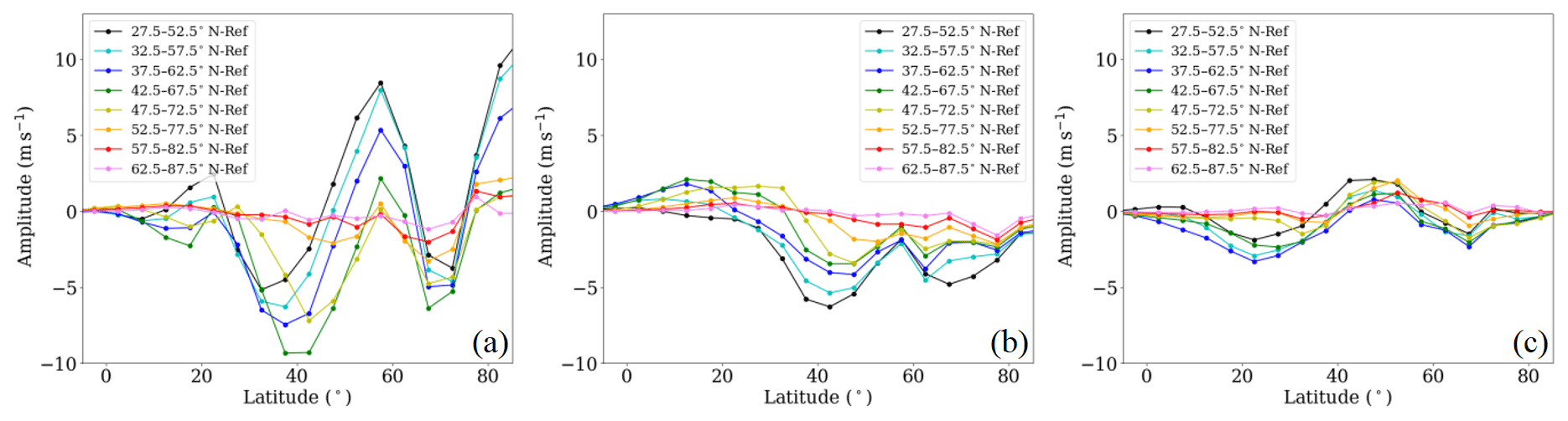
Figure 7 Zonal mean SPW 1 (a), SPW 2 (b) and SPW 3 (c) amplitudes as the difference between the H1–H8 simulations and the Ref simulation at 35 km for the last 30 d of the simulations extracted from the zonal wind.

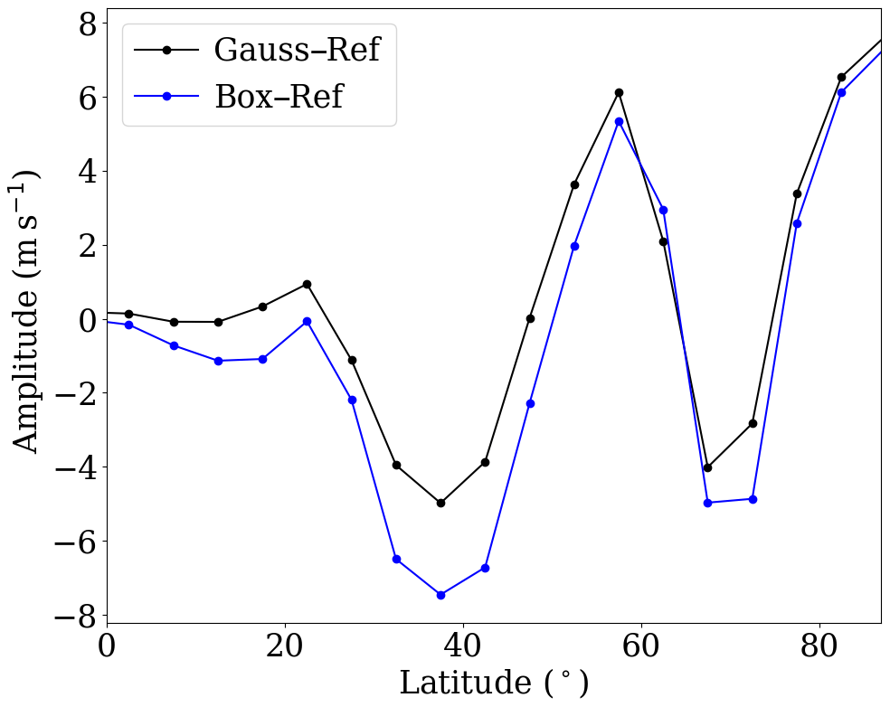
Figure 8 SPW 1 amplitude as the difference between the H3 simulation and the reference simulation (blue line) and the Gauss distribution and the reference simulation (black line) at 35 km for the last 30 d extracted from the zonal wind.

The suppression of SPWs, which is induced by the local GW forcing, might also be an effect partly induced by the shape of the GW hotspot, leading to a sharp transition zone between the unchanged and enhanced GW drag values. To prove that the shape of the GW hotspot partly leads to a suppression of SPWs, Fig. 8 shows the H3 amplitude anomaly from Fig. 7a and the corresponding Gauss simulation described in Sect. 2. The latitudinal distribution of the SPW 1 amplitude difference is still the same, showing the two local maxima at the midlatitudes and in the polar region and the two minima at 40 and 70^∘ N, although these two minima decreased from −8 m s⁻¹ for the 3-D box to −4 m s⁻¹ for the Gaussian distribution. Moreover, the maxima increased from about 4 m s⁻¹ to more than 5 m s⁻¹. Due to the stronger maximum GW drag in the Gaussian distribution the SPW 1 excitation is strengthened, which leads to the larger SPW 1 amplitudes at midlatitudes. The smoothly decreasing GW drag forcing towards lower and higher latitudes only slightly reduces the suppression of SPW 1 around 40 and 70^∘ N. The mean wind and temperatures are also only weakly affected if we replace the box-like forcing with one with a Gaussian shape (not shown here). Thus, the GW hotspot itself leads to essential changes in the dynamics, suppressing the SPW propagation and decreasing the SPW 1 activity in the middle atmosphere.

To sum up the influence on the polar vortex, in Sect. 3.1 we observed a slight warming of the lower stratosphere and a decreasing west wind at middle to high latitudes, which indicates a weakening of the polar vortex as a consequence of the GW drag enhancement. Thus, the stability of the polar vortex not only depends on the PW activity but also on the interplay or nonlinear interaction of GW and PW forcings. The anomalous SPW forcing and the suppression of SPW propagation show that the GW drag can play an important role in preconditioning the polar vortex (see next section).

3.3 Propagation conditions for SPWs

To establish the extent to which the SPW propagation is affected by the local GW forcing, the EP fluxes and their divergence for SPW 1 were calculated. The results of the Ref simulation are presented in Fig. 9a. The arrows show the direction of propagation, the color of the arrows represents the strength of the EP flux not normalized by the density, and the grey areas and the grey contour lines represent the EP divergence, showing the direction in which the zonal mean flow is accelerated. A negative (positive) EP divergence is illustrated by the dashed (solid) lines. The arrows were replaced by dots when the amplitude difference was smaller than 1 % of the maximum EP flux amplitude difference. The waves mainly develop in the middle and higher latitudes, and from there they mainly propagate towards the equatorial stratosphere/stratopause and, to a much lesser degree, to the polar stratosphere. That the waves are really propagating upwards can be seen by means of the increasing amplitudes of the EP fluxes. The maximum EP flux amplitudes of more than 1.4 m² s⁻² are reached between 50 and 60^∘ N at an altitude of about 60 km, which corresponds to the height of the SPW 1 amplitude maximum in Fig. 1f of the Ref simulation.

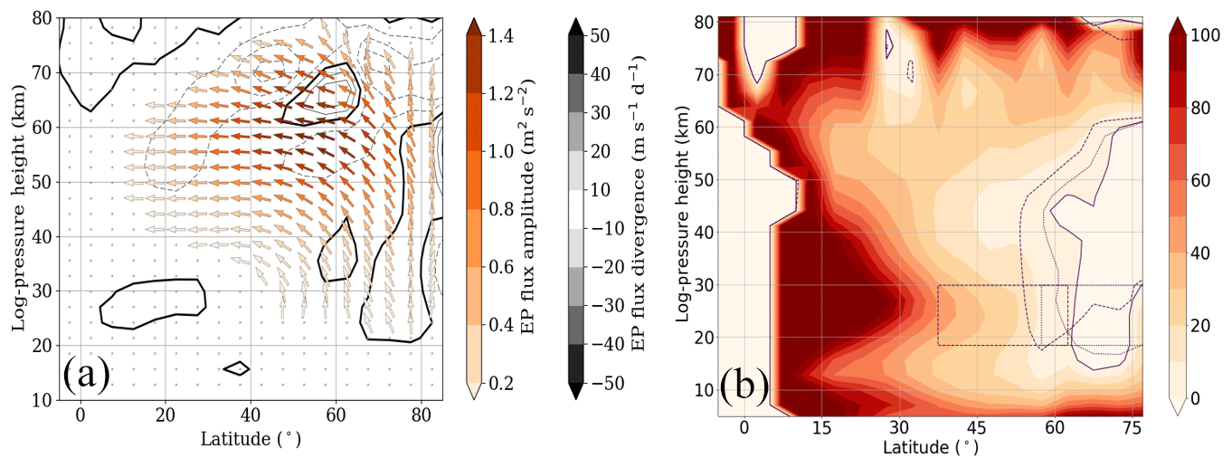
Figure 9 Zonal mean EP flux of SPW 1 of the Ref simulation (a). Contour lines show the EP flux divergence, and dashed lines denote negative EP flux divergence. The refractive index for SPW 1 for the Ref simulation (b) with a thicker zero line. The position of the H3 (H7) GW hotspot and the respective zero line is represented by the dashed (dotted) violet line. Both panels represent the last 30 d of the simulation.

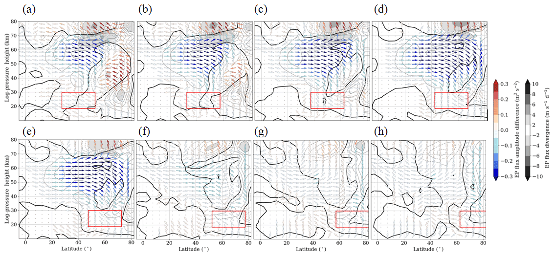
Figure 10 Zonal mean EP flux (arrows) and divergence (isolines and shaded areas; dashed lines show negative values) of SPW 1. Shown is the difference between all H1–H8 simulations (a–h) and the reference simulation (H1–H8 − Ref) representing the last 30 d of the simulations.

In Fig. 10 the difference in the EP flux and its divergence between the H1–H8 simulations and the Ref simulation is shown. The position of each GW hotspot is again illustrated by the red boxes. In the H1 and H2 simulations (Fig. 10a–b) more SPWs 1 propagate into the polar stratosphere. These SPWs 1 are partly coming from the midlatitudes but most of them are directly generated in the polar region, where we observe a source of SPWs 1 (enhanced positive EP divergence at 70^∘ N between 20 and 30 km). This positive EP divergence anomaly corresponds to the increased SPW 1 amplitude in the polar region in Fig. 7. Above this positive EP divergence anomaly an enhanced negative EP divergence is seen (from the northern flank of the GW hotspot up to 60 km tilted towards the north with increasing height), which means that the SPWs 1, which propagate via the Arctic stratosphere, break in this region. This leads to the deceleration of the zonal mean zonal wind in the middle and higher latitudes, as previously discussed in Fig. 3. The negative EP divergence anomaly can also be seen in the H3–H5 simulations (Fig. 10c–e). This is the reason why the polar vortex is mainly disturbed by these GW hotspots (H1–H5). The negative EP divergence is strongest for the H1 simulation, which also exhibits the strongest increase in SPW 1 amplitude in the polar region. Furthermore, the H1–H5 simulations show a strong decrease in the EP flux amplitude (blue arrows) between 40 and 70 km and between 20 and 80^∘ N, which means that fewer SPWs 1 are propagating into the middle atmosphere. As a consequence, fewer SPWs 1 break in this region, leading to a positive EP divergence anomaly. This result corresponds to the decreasing SPW 1 amplitude (Fig. 7) and the increasing zonal mean zonal wind (Fig. 3) at lower latitudes. The effect is strongest for the H4 simulation, which also shows the strongest decrease in SPW 1 amplitudes. Between 40 and 70^∘ N around 70 km we observe another source of SPWs 1, which propagate into the mesosphere, where these waves break (strongly negative EP divergence above the positive EP divergence) due to the reversed wind conditions. The mesospheric EP flux in the H1–H5 simulations corresponds to the observed enhanced SPW 1 amplitude in the mesosphere in Fig. 7. Referring to the enhanced SPW 1 around 55^∘ N of the GW hotspots, no enhanced EP flux can be observed in the respective region. However, the arrows of the EP flux anomalies are pointing towards this area of enhanced SPW 1 amplitude. In the H6–H8 GW hotspot simulations (Fig. 10f–h) no large differences in EP flux and divergence occur, which correspond to the small SPW 1 amplitude and the zonal mean zonal wind differences in Figs. 7 and 3.

Figure 11 Meridional potential vorticity gradient difference between the respective H3 (a)and H7 (b) simulations and the reference simulation, representing the last 30 d of the simulations. The positions of the H3 and H7 GW hotspots are represented by red boxes.

To explain why SPWs 1 do not propagate at higher latitudes, the refractive index (Matsuno, 1971; Andrews et al., 1987), multiplied by the square of the Earth's radius a², is also shown in Fig. 9b. The refractive index is highly dependent on the meridional potential vorticity gradient (q_y) and on the zonal mean zonal wind conditions (Li et al., 2007). White regions in Fig. 9b indicate a negative refractive index, which means that the waves cannot propagate in these regions. In the reddish regions wave propagation is possible. Due to the predominating westerly wind in the NH, the refractive index is mostly positive; therefore, SPWs 1 are able to propagate predominantly upward and towards the Equator. Towards the midlatitudes and the polar region the refractive index decreases due to the increasing zonal mean zonal wind. The polar region (north of 60^∘ N) is the only region in the NH with a negative refractive index. This is because the polar vortex is a strong closed system, which repels most of the waves. To establish the extent to which the refractive index changes after the implementation of the GW forcing, the position of the H3 (dashed violet line) and the H7 (dotted violet line) GW hotspot and the respective zero line of the refractive index were added to Fig. 9b. In the H3 simulation, the zero line is higher in the polar region than in the Ref simulation. Thus, the refractive index increases (becomes more positive) in the polar region below 30 km, which corresponds to the enhanced SPW 1 propagation and SPW 1 amplitude in the same region. The zero line of the H7 simulation is almost at the same height as that of the Ref simulation; thus, we do not observe huge changes in the Arctic. While the zero line of the Ref simulation is limited to the regions north of 60^∘ N, the zero line of the H3 (H7) simulation is located around 50^∘ N (57^∘ N). Based on the EP flux distribution of the Ref simulation in Fig. 9a, we already know that the SPWs 1 mainly propagate from the midlatitudes (between 50 and 60^∘ N) into the middle atmosphere. Due to the negative refractive index in this region, the SPWs 1 in the H3 and H7 simulations are no longer able to propagate upwards, meaning that the SPW 1 EP flux and amplitude decrease. Thus, the major branch of SPW 1 propagation is interrupted by the local GW forcing. To check if there are local instabilities leading to the SPW 1 sources in the polar region and in the lower mesosphere, the q_y differences between the H3 (H7) and the Ref simulation are shown in Fig. 11. The q_y is given in potential vorticity units (PVU) per degree. The positions of the H3 and H7 GW hotspot are illustrated using red boxes. Due to the increasing (decreasing) zonal mean zonal wind at lower (higher) latitudes, the q_y, which normally increases towards higher latitudes, is reversed northward of 30^∘ N. We observe a negative q_y anomaly, which is tilted towards the north with increasing height. Northward of 45^∘ N up to 20 km the q_y anomaly reverses again and becomes positive. These local reversals of the q_y, which are a necessary condition for baroclinic instability (Charney and Stern, 1962), can lead to the SPW 1 sources and positive EP divergences in the respective regions.

4 Conclusions

The sensitivity study regarding the effect of local GW hotspots in the stratosphere from lower to higher latitudes in a specific longitude range (between 120 and 170^∘ E) shows that GW hotspots south of 50^∘ N lead to a negative refractive index at midlatitudes, which prevents the SPWs from propagating upwards. Thus, fewer SPWs 1 are breaking in the middle atmosphere corresponding to the decreasing SPW 1 amplitude at lower latitudes connected with an increasing zonal mean zonal wind. Thus, the polar vortex is shifted towards lower latitudes but remains very strong (Baldwin and Holton, 1988), which additionally leads to a suppression of SPWs according to the Charney–Drazin criterion (Charney and Drazin, 1961). The displacement of the polar vortex induced by breaking SPWs 1 causes an increase in the refractive index in the polar stratosphere (Karami et al., 2016); thus, the SPWs 1 originating at midlatitudes partly propagate via the polar region into the middle atmosphere. Apart from these SPWs 1, additional SPWs 1 propagating upwards are directly generated in the Arctic owing to local baroclinic instability; one indication of this is the reversal of the q_y (Charney and Stern, 1962; Garcia, 1991). For this reason we observe an enhanced EP flux and, thus, an enhanced SPW 1 amplitude in the polar region. These SPWs 1 break around 50 km between 50 and 80^∘ N and lead to an enhanced negative EP divergence connected with a decrease in zonal mean zonal wind at higher latitudes. In the lower mesosphere between 40 and 70^∘ N there is a second source of SPWs 1 (positive EP divergence) in addition to local baroclinic instabilities (reversal of the q_y) (Smith, 2003; Lieberman et al., 2013; Matthias and Ern, 2018). As a consequence, the EP flux and the SPW 1 amplitude are enhanced between 70 and 80 km, right above the positive EP divergence anomaly. Based on the SPW 1 amplitude extracted from the zonal GW drag (not shown here) it was clear that each of the GW hotspots leads to a forcing of SPWs 1, but in some regions northward of 50^∘ N this forcing is ineffective because the waves cannot propagate or are eliminated by destructive interference. The refractive index, which is highly dependent on the zonal mean zonal wind conditions, shows negative values in the polar region for the Ref simulation. Thus, if we implement a GW forcing directly in this region it has no impact on the middle atmosphere as SPWs cannot propagate. If we provoke preconditioning of the polar vortex by first implementing, for example, the H1 GW hotspot and then adding one of the H6–H8 GW hotspots, the GW hotspots near the polar region would have a larger impact on the dynamics of the middle atmosphere.

Based on the results of the sensitivity study, we see that a local GW forcing can lead to a weakening (warming of the lower stratosphere) and slight displacement of the polar vortex at high latitudes, which is highly dependent on the strength (Šácha et al., 2016) and the zonal distribution of the forcing (this study). Usually, it is assumed that preconditioning of the polar vortex is mainly driven by enhanced PW activity (Labitzke, 1981). However, there are also several indications based on satellite observations (Ern et al., 2016) and reanalysis data (Albers and Birner, 2014) which show that the GW drag and the absolute GW momentum flux is enhanced (reduced) in the stratosphere right before (after) SSWs. Albers and Birner (2014) analyzed the total wave forcing from the Japanese Meteorological Agency and Central Research Institute of Electrical Power Industry 25-year Reanalysis (JRA-25) data before SSW events and found that up to 70 % of the total drag is induced by orographic GWs. Ern et al. (2016) directly derived the GW drag and absolute momentum fluxes from HIRDLS and SABER temperatures and found that both parameters are enhanced before and around the central day of a SSW (strong polar jet), and they are reduced when the zonal wind is weak (after SSW). Because we kept the GW drag forcing constant throughout the experiment we cannot evaluate nonlinear effects, which would possibly reduce the GW drag connected with the displacement of the polar vortex. Furthermore, we have a fixed GW source distribution, meaning that no additional GWs are generated owing to changes in the tropospheric circulation. Nevertheless, on the basis of the zonal and meridional GW flux, which changes according to the propagation conditions, we analyzed the absolute horizontal GW momentum flux (not shown here). In this case, we also observe a reduction in the GW flux when the zonal mean zonal wind decreases at high latitudes. However, this effect is not very pronounced in our experiments, as the zonal mean zonal wind differences are much smaller than during a real SSW event. We only observe zonal mean zonal wind differences of about −10 m s⁻¹, which do not lead to a reversal of the zonal mean zonal wind or to subsequent significant background changes that may strongly influence the GW propagation.

Another interesting aspect is that different local GW forcing shapes do not have strong effects on the circulation. In spite of the Gaussian-smoothed boundaries, only negligible changes can be observed in the dynamics and SPW development, which are mainly due to the varying GW drag in the 3-D Gaussian distribution, leading to larger (smaller) effects when the Gaussian distribution reaches a maximum (minimum).

Comparing the positions of these simulated GW hotspots with measurements (e.g., Hoffmann et al., 2013), it is clear that at least some of the latitudinally shifted GW hotspots are not very realistic; therefore, our experiments should only be considered as a qualitative sensitivity study. Regarding orography, there are no obvious sources of orography when we displace the GW hotspot latitudinally. However, some of the GW hotspots can connect to jet exit regions on a purely hypothetical basis. To make the study more realistic, the next step would be to analyze the effect of a longitudinally shifted hotspot (fixed latitude range between 30 and 60^∘ N), as observations and GCM experiments have shown their existence (listed in the introduction). In this latitude range GW hotspots like the Himalayan region, the Alps or the Rocky mountains are included in the experiments. Also, the interaction of two or more GW hotspots is one of our focuses and will provide more insight into the effect of a localized GW forcing, which may be also important for the development of new GW parameterizations.

Appendix A

Figure A1 Zonal mean EP flux (arrows) and divergence (isolines and shaded areas; dashed lines show negative values) of SPW 1. Shown is the difference between all H1–H8 (a–h) simulations and the reference simulation (H1–H8 − Ref) representing the last 30 d of the simulations. The EP flux is weighted by the density.