Local time extent of magnetopause reconnection using space–ground coordination

Magnetic reconnection can vary considerably in spatial extent. At the Earth's magnetopause, the extent generally corresponds to the extent in local time. The extent has been probed by multiple spacecraft crossing the magnetopause, but the estimates have large uncertainties because of the assumption of spatially continuous reconnection activity between spacecraft and the lack of information beyond areas of spacecraft coverage. The limitations can be overcome by using radars examining ionospheric flows moving anti-sunward across the open–closed field line boundary. We therefore infer the extents of reconnection using coordinated observations of multiple spacecraft and radars for three conjunction events. We find that when reconnection jets occur at only one spacecraft, only the ionosphere conjugate to this spacecraft shows a channel of fast anti-sunward flow. When reconnection jets occur at two spacecraft and the spacecraft are separated by < 1 Re, the ionosphere conjugate to both spacecraft shows a channel of fast anti-sunward flow. The consistency allows us to determine the reconnection jet extent by measuring the ionospheric flows. The full-width-at-half-maximum flow extent is 200, 432, and 1320 km, corresponding to a reconnection jet extent of 2, 4, and 11 Re. Considering that reconnection jets emanate from reconnections with a high reconnection rate, the result indicates that both spatially patchy (a few Re) and spatially continuous and extended reconnections (> 10 Re) are possible forms of active reconnection at the magnetopause. Interestingly, the extended reconnection develops from a localized patch via spreading across local time. Potential effects of IMF B_x and B_y on the reconnection extent are discussed.

1 Introduction

A long-standing question in magnetic reconnection is the following: what is the spatial extent of reconnection in the direction normal to the reconnection plane? At the Earth's magnetopause, for a purely southward IMF, this corresponds to the extent in the local time or azimuthal direction. The extent of reconnection has significant relevance to solar wind–magnetosphere coupling, as it controls the amount of energy being passed through the boundary from the solar wind into the magnetosphere and ionosphere. Magnetopause reconnection tends to occur at sites of strictly antiparallel magnetic fields as antiparallel reconnection (e.g., Crooker, 1979; Luhmann et al., 1984) or along a line passing through the subsolar region as component reconnection (e.g., Sonnerup, 1974; Gonzalez and Mozer, 1974). Evidence shows either or both can occur at the magnetopause, and the overall reconnection extent can span from a few to 40 Re (Paschmann et al., 1986; Gosling et al., 1990; Phan and Paschmann, 1996; Coleman et al., 2001; Phan et al., 2000b, 2003; Chisham et al., 2002, 2004a, 2008; Petrinec and Fuselier, 2003; Fuselier et al., 2002, 2003, 2005, 2010; Pinnock et al., 2003; Bobra et al., 2004; Trattner et al., 2004, 2007, 2008, 2017; Trenchi et al., 2008). However, reconnection does not occur uniformly across this configuration but has spatial variations (Pinnock et al., 2003; Chisham et al., 2008), and it is reconnection with high reconnection rates that effectively contributes to the momentum and energy flow within the magnetosphere. Reconnection with high reconnection rates is expected to cause rapid magnetic flux generation and fast reconnection jets. This paper therefore investigates the spatial extent of reconnection through the extent of reconnection jets.

Numerical models show that reconnection tends to occur at magnetic separators, i.e., at the junction between regions of different magnetic field topologies, and global magnetohydrodynamics (MHDs) models have identified a spatially continuous separator along the magnetopause (Dorelli et al., 2007; Laitinen et al., 2006, 2007; Haynes and Parnell, 2010; Komar et al., 2013; Glocer et al., 2016). However, little is known about where and over what range along the separators reconnection proceeds at a high rate. Reconnection in numerical simulations can be activated by introducing perturbations of the magnetic field or can grow spontaneously with instability or resistivity inherent in the system (e.g., Hesse et al., 2001; Scholer et al., 2003). When reconnection develops as patches (due to instabilities or localized perturbations), the patches can spread in the direction out of the reconnection plane (Huba and Rudakov, 2002; Shay et al., 2003; Lapenta et al., 2006; Nakamura et al., 2012; Shepherd and Cassak, 2012; Jain et al., 2013). The patches either remain patchy after spreading if the current layer is thick or form an extended X line if the current layer is already thin (Shay et al., 2003).

Studies have attempted to constrain the extent of reconnection based on fortuitous satellite conjunctions whereby the satellites detect reconnection jets at the magnetopause at different local times nearly simultaneously (Phan et al., 2000a, 2006; Walsh et al., 2014a, b, 2017). The satellites were separated by a few Re in Phan et al. (2000a) and Walsh et al. (2014a, b, 2017) and > 10 Re in Phan et al. (2006), and this is interpreted as the reconnection being active over a few Re and even 10 Re, respectively. At the magnetopause, reconnection of a few Re is often referred to as spatially patchy (e.g., Fear et al., 2008, 2010), and reconnection of > 10 Re is spatially extended (Dunlop et al., 2011; Hasegawa et al., 2016). The term patchy has also been used to describe the temporal characteristics of reconnection (e.g., Newell and Meng, 1991). But this paper primarily focuses on the spatial properties. The extent has been alternatively determined by studying the structures of newly reconnected flux tubes, i.e., flux transfer events (FTEs) (Russell and Elphic, 1979; Haerendel et al., 1978). Conceptual models regard FTEs either as azimuthally narrow flux tubes that intersect the magnetopause through nearly circular holes, as formed by spatially patchy reconnection (Russell and Elphic, 1979), or as azimuthally elongated bulge structures or flux ropes that extend along the magnetopause, as formed by spatially extended reconnection (Scholer, 1988; Southwood et al., 1988; Lee and Fu, 1985). FTEs have been observed to be on the order of a few Re wide in local time (Fear et al., 2008, 2010; Wang et al., 2005, 2007). FTEs have also been observed across ∼20 Re from the subsolar region to the flanks (Dunlop et al., 2011). But it is unclear whether these FTEs are branches of one extended bulge or flux rope or multiple narrow tubes formed simultaneously. When the satellites are widely spaced, it is in general questionable whether a reconnection jet and/or FTE is spatially continuous between the satellites or whether satellites detect the same moving reconnection jet and/or FTE. Satellites with a small separation may possibly measure the same reconnection jet and/or FTE, but only provide a lower limit estimate of the extent. A reconnection jet and/or FTE may also propagate or spread between satellite detections, but satellite measurements cannot differentiate spatial and temporal effects.

This situation can be improved by studying ionospheric signatures of reconnection and FTEs, since their spatial sizes in the ionosphere can be obtained from wide-field ground instruments or low-Earth-orbit spacecraft. The ionospheric signatures include poleward-moving auroral forms (PMAFs), channels of flows moving anti-sunward across the open–closed field line boundary (e.g., Southwood, 1985), and cusp precipitation (Lockwood and Smith, 1989, 1994; Smith et al., 1992). Radar studies have shown that the flows can differ considerably in size, varying from tens of kilometers (Oksavik et al., 2004, 2005) to hundreds of kilometers (Goertz et al., 1985; Pinnock et al., 1993, 1995; Provan and Yeoman, 1999; Thorolfsson et al., 2000; McWilliams et al., 2000b, 2001) or thousands of kilometers (Provan et al., 1998; Nishitani et al., 1999; Provan and Yeoman, 1999). A similarly broad distribution has been found for PMAFs (e.g., Sandholt et al., 1986, 1990; Lockwood et al., 1989, 1990; Milan et al., 2000, 2016) and the cusp (Crooker et al., 1991; Newell and Meng, 1994; Newell et al., 2007). This range of spatial sizes in the ionosphere approximately corresponds to a range from < 1 to > 10 Re at the magnetopause. However, care needs to be taken when interpreting the above ionospheric features, since they could also form due to other drivings such as solar wind dynamic pressure pulses (Lui and Sibeck, 1991; Sandholt et al., 1994). Unambiguous proof of their connection to magnetopause reconnection requires simultaneous space–ground coordination (Elphic et al., 1990; Denig et al., 1993; Neudegg et al., 1999, 2000; Lockwood et al., 2001; Wild et al., 2001, 2005, 2007; McWilliams et al., 2004; Zhang et al., 2008).

Therefore, a reliable interpretation of reconnection extent has been difficult due to observation limitations. We will address this by comparing the extents probed by multiple spacecraft and radars using space–ground coordination. On the one hand, this enables us to investigate whether reconnection continuously spans between satellites and how wide reconnection extends beyond satellites. On the other hand, this helps to determine whether reconnection is the driver of ionospheric disturbances and whether the in situ extent is consistent with the ionospheric disturbance extent.

2 Methodology

We study the characteristic extent of reconnection jets as the local time extent of reconnection. We use conjugate measurements between the Time History of Events and Macroscale Interactions during Substorms (THEMIS) (Angelopoulos, 2008) and Super Dual Auroral Network (SuperDARN) (Greenwald et al., 1995). We focus on intervals when the IMF in OMNI data remains steadily southward. We require that two of the THEMIS satellites fully cross the magnetopause nearly simultaneously and that the satellite data provide clear evidence for reconnection occurring or not. The full crossings are identified by a reversal of the B_z magnetic field and a change in the ion energy spectra. The requirements of nearly simultaneous crossings and steady IMF conditions help to reduce the spatial–temporal ambiguity by satellite measurements, for which the presence and absence of reconnection jets at different local times likely reflects spatial structures of reconnection. Reconnection can still possibly vary between the two satellite crossings, and we use the radar measurements to examine whether the reconnection of interest has continued to exist and maintained its spatial size.

Identification of reconnection jets in the magnetosphere is based on fluid (MHD) evidence of magnetopause reconnection. Reconnection accelerates plasma bulk flow to Alfvénic speed, producing reconnection jets at the magnetopause, and the acceleration should be consistent with the prediction of tangential stress balance across a rotational discontinuity, i.e., the Walen relation (Hudson, 1970; Paschmann et al., 1979). The Walen relation is expressed as

$$\begin{array}{ll}{\displaystyle }\mathrm{\Delta }{V}_{\mathrm{predicted}}=& {\displaystyle }\pm {\left(\mathrm{1}-{\mathit{\alpha }}_{\mathrm{1}}\right)}^{\mathrm{1}/\mathrm{2}}{\left({\mathit{\mu }}_{\mathrm{0}}{\mathit{\rho }}_{\mathrm{1}}\right)}^{-\mathrm{1}/\mathrm{2}}\\ \text{(1)}& {\displaystyle }& {\displaystyle }\left[B_{\mathrm{2}}\left(\mathrm{1}-{\mathit{\alpha }}_{\mathrm{2}}\right)/\left(\mathrm{1}-{\mathit{\alpha }}_{\mathrm{1}}\right)-B_{\mathrm{1}}\right],\end{array}$$

where ΔV is the change in the plasma bulk velocity vector across the discontinuity. B and ρ are the magnetic field vector and plasma mass density. μ₀ is the vacuum permeability. $\mathit{\alpha }=(p_{\mathrm{|}\mathrm{|}}-p_{\perp }){\mathit{\mu }}_{\mathrm{0}}/B^{\mathrm{2}}$ is the anisotropy factor wherein p_|| and p_⊥ are the plasma pressures parallel and perpendicular to the magnetic field. The magnetic field and plasma moments are obtained from fluxgate magnetometer (FGM) (Auster et al., 2008) and electrostatic analyzer (ESA) instruments (McFadden et al., 2008). The plasma mass density is determined using the ion number density, assuming a mixture of 95 % protons and 5 % helium. The subscripts 1 and 2 refer to the reference interval in the magnetosheath and to a point within the magnetopause, respectively. The magnetosheath reference interval is a 10 s time period just outside the magnetopause. The point within the magnetopause is taken at the maximum ion velocity change across the magnetopause. We ensure that the plasma density at this point is > 20 % of the magnetosheath density to avoid the slow-mode expansion fan (Phan and Paschmann, 1996). We compare the observed ion velocity change with the prediction from the Walen relation. The level of agreement is measured by $\mathrm{\Delta }{V}^{*}=\mathrm{\Delta }{V}_{\mathrm{obs}}\cdot \mathrm{\Delta }{V}_{\mathrm{predicted}}/|\mathrm{\Delta }{V}_{\mathrm{predicted}}{|}^{\mathrm{2}}$, following Paschmann et al. (1986). Here ΔV_obs is the observed ion velocity change. B_y convention only the velocity changes with $\mathrm{\Delta }{V}^{*}>\mathrm{0.5}$ are classified as reconnection jets (e.g., Phan et al., 1996; Phan and Paschmann, 2013).

To further ensure that reconnection occurs, we examine the kinetic signature of reconnection, which is D-shaped ion distributions at the magnetopause. As magnetosheath ions encounter newly opened magnetic field lines at the magnetopause, they either transmit through the magnetopause entering the magnetosphere or reflect at the boundary. The transmitted ions have a cutoff parallel velocity (i.e., de Hoffmann–Teller velocity) below which no ions could enter the magnetosphere. The D-shaped ion distributions are deformed into a crescent shape as ions travel away from the reconnection site (Broll et al., 2017). We require the satellites to operate in the fast survey or burst mode in which ion distributions are available at 3 s resolution.

We determine reconnection as active if the plasma velocity change across the magnetopause is consistent with the Walen relation with $\mathrm{\Delta }{V}^{*}\mathit{>}=\mathrm{0.5}$ and if the ions at the magnetopause show a D-shaped distribution. Reconnection is deemed absent if neither of the two signatures is detected. We require that at least one of the two satellites observes reconnection signatures. Reconnection is regarded as ambiguous if only one of the two signatures is detected, and such reconnection is excluded from our analysis.

We mainly use the three SuperDARN radars located at Rankin Inlet (RKN; geomagnetic 72.6^∘ MLAT, −26.4^∘ MLON), Inuvik (INV; 71.5^∘ MLAT, −85.1^∘ MLON), and Clyde River (CLY; 78.8^∘ MLAT, 18.1^∘ MLON) to measure the ionospheric convection near the dayside cusp. The three radars have overlapping fields of view (FOVs), enabling a reliable determination of the 2-D convection velocity. The FOVs cover the ionosphere > 75^∘ MLAT, covering the typical location of the cusp under weak and modest solar wind driving conditions (i.e., Newell et al., 1989) and the high occurrence region of reconnection-related ionospheric flows (Provan and Yeoman, 1999) with high spatial resolution. Data from Saskatoon (SAS; 60^∘ MLAT, −43.8^∘ MLON) and Prince George (PGR; 59.6^∘ MLAT, −64.3^∘ MLON) radars are also used when data are available. The measurements of these two radars at far-range gates can overlap the cusp. The radar data have a time resolution of 1–2 min. We focus on observations ±3 h MLT from magnetic noon (approximately 16:00–22:00 UT). The satellite footprints should be mapped close to the radar FOVs under the Tsyganenko (T89) model (Tsyganenko, 1989). Footprints mapped using different Tsyganenko (e.g., T96 or T01; Tsyganenko, 1995, 2002a, b) models have similar longitudinal locations (difference < 100 km), implying the longitudinal uncertainty of mapping to be small. The latitudinal uncertainty can be inferred by referring to the open–closed field line boundary as estimated using the 150 m s⁻¹ spectral width boundary (e.g., Baker et al., 1995, 1997; Chisham and Freeman, 2003). T89 has given the smallest latitudinal uncertainty for the studied events. We surveyed the years 2014–2016 during the months when the satellite apogee was on the dayside and present three events in the paper.

The ionospheric signature of reconnection jets includes fast anti-sunward flows moving across the open–closed field line boundary. We obtain the flow velocity vectors by merging line-of-sight (LOS) measurements at the radar common FOVs (Ruohoniemi and Baker, 1998), and these merged vectors reflect the true ionospheric convection velocity. However, the radar common FOVs are hundreds of kilometers wide only, which can be too small to cover the full azimuthal extent of the reconnection-related flows (which are up to thousands of kilometers wide). We therefore also reconstruct the velocity field using the spherical elementary current system (SECS) method (Amm et al., 2010). Similar to the works by Ruohoniemi et al. (1989) and Bristow et al. (2016), the SECS method reconstructs a divergence-free flow pattern using all LOS velocity data. We refer to these velocities as SECS velocities. The accuracy of SECS velocities can be validated by comparing to the LOS measurements and the merged vectors. SECS velocities work best in regions with dense echo coverage, and those around sparse echoes are not reliable and thus are excluded from our analysis.

The third way of obtaining a velocity field is spherical harmonic fit (SHF). This method uses the LOS measurements and a statistical convection model to fit the distribution of electrostatic potential, which is expressed as a sum of spherical harmonic functions (Ruohoniemi and Baker, 1998). The statistical model employed here is from Cousins and Shepherd (2010). While this method may suppress small-scale or mesoscale velocity details, such as sharp flow gradients or flow vortices, we compare SHF velocities with the LOS measurements and merged vectors to determine how well the SHF velocities depict the velocity details.

As seen in our observations presented below, the longitudinal profile of the fast anti-sunward ionospheric flows has a nearly bell-shaped curve. We measure the extent based on the full width at half maximum (FWHM) of the profile at 1^∘ poleward of the open–closed field line boundary. The choice of FWHM is analogous to Shay et al. (2003), in which the reconnection extent is measured as regions of electron speed above half of the peak electron flow speed during reconnection. The choice is also supported by magnetopause observations, in which we find that ionospheric flows with a speed above half of the peak flow speed map to jets consistent with the Walen relation, while those with a speed below map to jets much slower than the Walen relation (Sect. 3.1). However, it should be noted that the magnitude of the widths is always dependent on the threshold used, and the half maximum is very likely not the only sensible threshold. Using FWHM excludes ionospheric flows with a speed below half of the peak flow speed. Those flows, if related to reconnection, are associated with the comparatively slow generation of open magnetic flux and a low contribution to geomagnetic activity.

Among the three presented events, the time separations of magnetopause crossings by two satellites are 1, 2, and 30 min. While the time separation for the third case is somewhat long, we distinguish spatial and temporal effects using the radar data. Although the three events occurred under similar IMF B_z conditions, the reconnection-related flows in the ionosphere had an azimuthal extent varying from a few hundred kilometers (Sect. 3.1–3.2) to more than 1000 km wide (Sect. 3.3). This corresponds to reconnection a few to > 10 Re wide, indicating that both spatially patchy (a few Re) and spatially continuous and extended reconnections (> 10 Re) are possible forms of active reconnection at the magnetopause. Interestingly, the extended reconnection was found to arise from a spatially localized patch that spreads azimuthally. Potential effects of IMF B_x and B_y on the reconnection extent are discussed in Sect. 4.

Note that reconnection can happen over various spatial and temporal scales and our space–ground approach can resolve reconnections that are larger than 0.5 Re and persist longer than a few minutes. This is limited by the radar spatial and temporal resolution and the magnetosphere–ionosphere coupling time, which is usually 1–2 min (e.g., Carlson et al., 2004). This constraint is not expected to impair the result because reconnection above this scale has been found to occur commonly in statistics (see the Introduction for spatial characteristics and the following for temporal characteristics: Lockwood and Wild, 1993; Kuo et al., 1995; Fasel, 1995; McWilliams et al., 2000a).

3 Observations

3.1 Spatially patchy reconnection active at one satellite only

3.1.1 In situ satellite measurements

On 2 February 2013, THA and THE made simultaneous measurements of the dayside magnetopause with a 1.9 Re separation in the Y direction around 21:25 UT. The IMF condition is displayed in Fig. 1a and the IMF was directed southward. The satellite location in GSM coordinates is displayed in Fig. 1b, and the measurements are presented in Fig. 2. The magnetic field and the ion velocity components are displayed in the LMN boundary-normal coordinate system, wherein L is along the outflow direction, M is along the X line, and N is the current sheet normal. The coordinate system is obtained from the minimum variance analysis of the magnetic field at each magnetopause crossing (Sonnerup and Cahill Jr., 1967). Figure 2g–p show that both satellites passed from the magnetosheath into the magnetosphere, as seen as the sharp changes in the magnetic field, the ion spectra, and the density (shaded in pink).

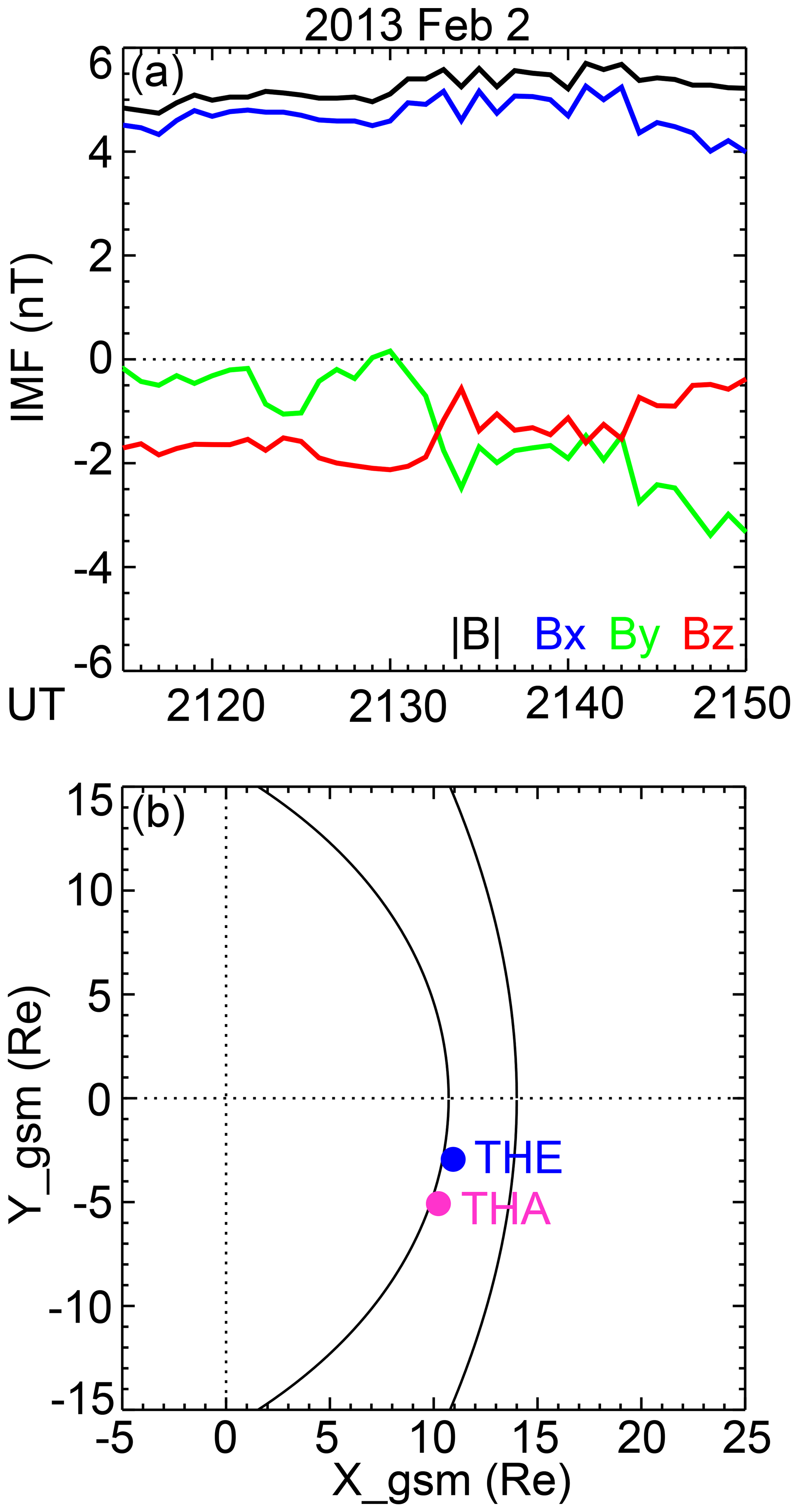
Figure 1 (a) OMNI IMF condition on 2 February 2013. (b) THE and THA locations projected to the GSM X–Y plane. The inner curve marks the magnetopause and the outer curve marks the bow shock.

As THE crossed the magnetopause boundary layer (21:22:57–21:23:48 UT), it detected a rapid, northward-directed plasma jet within the region where the magnetic field rotated (Fig. 2g and j). The magnitude of this jet relative to the sheath background flow reached 262 km s⁻¹ at its peak, which was 72 % of the predicted speed of a reconnection jet by the Walen relation (366 km s⁻¹, not shown). The angle between the observed and predicted jets was 39^∘. THE also detected kinetic signatures of reconnection. The ion distributions in Fig. 2k show a distorted D-shaped distribution similar to the finding of Broll et al. (2017). The distortion is due to particles traveling in the field-aligned direction from the reconnection site to a stronger magnetic field region, and Broll et al. (2017) estimated the traveling distance to be a few Re for the observed level of distortion.

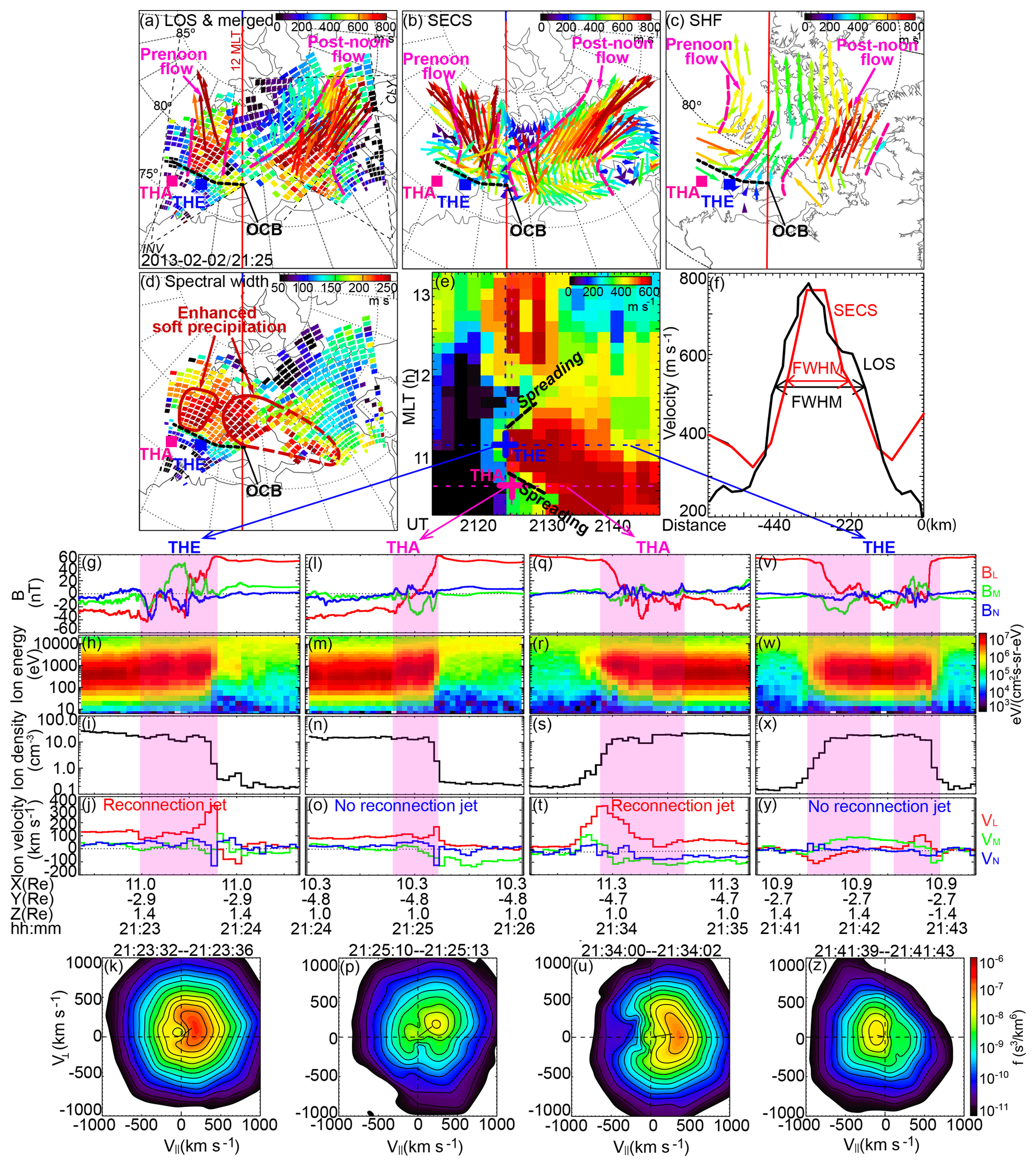
Figure 2 (a) SuperDARN LOS speeds (color tiles) and merged velocity vectors (color arrows) in the altitude-adjusted corrected geomagnetic (AACGM) coordinates. The FOVs of the RKN, INV, and CLY radars are outlined with black dashed lines. The colors of the tiles indicate the LOS speeds away from the radar. The colors and the lengths of the arrows indicate the merged velocity magnitudes, and the arrow directions indicate the velocity directions. Red and anti-sunward-directed flows are the ionospheric signature of magnetopause reconnection. The dashed magenta lines mark the flow western and eastern boundaries. The open–closed field line boundary is delineated by the dashed black curve with the OCB marker. The satellite footprints under the T89 are shown as the THE and THA markers. (b) Similar to (a) but showing SECS velocity vectors (color arrows). (c) Similar to (a) but showing SHF velocity vectors (color arrows). (d) SuperDARN spectral width measurements (color tiles). The red contour marks localized enhanced soft electron precipitation. (e) Time evolution of the northward component of SECS velocities along 79^∘ MLAT. (f) Profile of convection velocities along 79^∘ MLAT at 21:29 UT as a function of the distance from magnetic noon. The profile in black is based on the LOS measurements, and the profile in red is the northward component of the SECS velocities. The FWHM is determined based on each profile. (g–j) THE measured magnetic field (0.25 s resolution), ion energy flux (3 s), ion density (3 s), and ion velocity (3 s). The ion measurements were taken from ground ESA moments. The magnetic field and the ion velocity components are displayed in the LMN boundary-normal coordinate system. The magnetopause crossing is shaded in pink. (k) THE ion distribution function on the bulk velocity–magnetic field plane. The small black line indicates the direction and the bulk velocity of the distributions. (l–p) THA measurements in the same format as in (g)–(k). (q–z) THA and THE measurements during a subsequent magnetopause crossing shown in the same format as in (g)–(p).

THA crossed the magnetopause 1 to 2 min later than THD (21:24:48–21:25:13 UT). While it still identified a plasma jet at the magnetopause (Fig. 2l and o), the jet speed was significantly smaller than what was predicted for a reconnection jet (80 km s⁻¹ versus 380 km s⁻¹ in the L direction). The observed jet was directed 71^∘ away from the prediction. The ion distributions deviated from clear D-shaped distributions (Fig. 2p). This suggests that the reconnection jet at THE likely did not extend to THA.

3.1.2 Ground radar measurements

The velocity field of the dayside cusp ionosphere during the satellite measurements is shown in Fig. 2a–c. Figure 2a shows the radar LOS measurements at 21:25 UT, as denoted by the color tiles, and the merged vectors, as denoted by the arrows. The colors of the arrows indicate the merged velocity magnitudes, and the colors of the tiles indicate the LOS speeds that direct anti-sunward (those projected to the sunward direction appear as black). Fast (red) and anti-sunward flows are the feature of interest here. One such flow can be identified in the prenoon sector, which had a speed of ∼800 m s⁻¹ and was directed poleward and westward. As the merged vector arrows indicate, the velocity vectors have a major component close to the INV beam directions, and thus the INV LOS velocities reflect the flow distribution. The flow crossed the open–closed field line boundary, which was located at 78^∘ MLAT based on the spectral width (Figs. 2d and S1 in the Supplement). This flow thus meets the criteria for being an ionospheric signature of magnetopause reconnection jets. Another channel of fast flow was present in the post-noon sector. This post-noon flow was directed more azimuthally and was increasingly separated from the prenoon flow as it moved away from noon (see the region of slow velocities at > 79^∘ MLAT around noon). The difference in flow trajectories implies that these flows were driven by different magnetic tension forces. They also evolved differently over time as seen in Fig. 2e, which is discussed below. The flows thus likely originated from two reconnection regions that were associated with different magnetic field topologies and different temporal variabilities. Since the satellites were located in the prenoon sector we focus on the prenoon flow below.

The flow had a limited azimuthal extent. The extent is determined at half of the maximum flow speed, which was ∼400 m s⁻¹. Figure 2f, discussed below, shows a more quantitative estimate of the extent. In Fig. 2a, we mark the eastern and western boundaries with dashed magenta lines, across which the LOS velocities dropped from red to blue–green.

Figure 2b shows the SECS velocities, denoted by the arrows. The SECS velocities reasonably reproduced the spatial structure of the flows seen in Fig. 2a. The flow boundaries are marked by dashed magenta lines, across which the flow speed dropped from red to blue.

The velocity field reconstructed using the SHF velocities is shown in Fig. 2c (obtained through the Radar Software Toolkit; http://superdarn.thayer.dartmouth.edu/software.html, last access: March 2018). This is an expanded view of the global convection maps in Fig. S2 focusing on the dayside cusp. Comparing Figs. 2c and S2 reveals that the employed radars listed in Sect. 2 have contributed to the majority of the backscatter on the dayside. This is because this event (the same for the following two events) occurred under non-storm time, wherein the open–closed field line was confined within the FOVs of the radars used. During storm time the boundary expands to a lower latitude at which backscatter from a wider network of radars may be available. The SHF velocities also captured the occurrence of two flows in the prenoon and post-noon sectors, respectively, although the orientation of the flows was slightly different from Fig. 2a or b. The difference is likely due to the contribution from the statistical potential distribution under the southward IMF. The flow western and eastern boundaries are again marked by dashed magenta lines.

Figure 2d shows spectral width measurements. Large spectral widths can be produced by soft (∼100 eV) electron precipitation (Ponomarenko et al., 2007), and evidence has shown that the longitudinal extent of large spectral widths correlates with the extent of PMAFs (Moen et al., 2000) and of poleward flows across the open–closed field line boundary (Pinnock and Rodger, 2000). Large spectral widths thus have the potential to reveal the reconnection extent. For the specific event under examination, the region of large spectral widths, appearing in red, spanned from 10.5 to 14.5 h MLT if we count the sporadic scatter in the post-noon sector. This does not contradict the flow width identified above because the wide width reflects the summed width of the prenoon and post-noon flows. In fact, a more careful examination shows that there might be two dark red regions (circled in red; the red dashed line is due to the discontinuous backscatter outside the INV FOV) embedded within the ∼200 m s⁻¹ spectral widths. These two regions had slightly higher spectral widths than the surrounding regions (by ∼20–50 m s⁻¹) and possibly corresponded to the two flows.

Figures 2a–c all show a channel of fast anti-sunward flow in the prenoon sector of the high-latitude ionosphere, and the flow had a limited azimuthal extent. If the flow corresponded to a magnetopause reconnection jet, the reconnection jet would be expected to span a limited local time range. This is consistent with the THEMIS satellite observation in Sect. 3.1.1, in which THE at $Y=-\mathrm{2.9}$ Re detected a clear reconnection jet, while THA at $Y=-\mathrm{4.8}$ Re did not. In fact, if we project the satellite location to the ionosphere through field line tracing under the T89 model, THE was positioned at the flow longitude, while THA was to the west of the flow embedded in weak convection (Fig. 2a).

While this paper primarily focuses on the spatial extent of reconnection, the temporal evolution can be obtained from the time series plot in Fig. 2e. Figure 2e presents the northward component of the SECS velocity along 79^∘ MLAT (just 1^∘ poleward of the open–closed field line boundary) as a function of magnetic local time (MLT) and time. Here we only show the northward component of the SECS velocity as this component represents reconnecting flows across an azimuthally aligned open–closed field line boundary. Similar to the snapshots, the flow of interest here appears as a region of red. The time and the location where THA and THE crossed the magnetopause are marked by crosses. The prenoon flow emerged from a weak background from 21:22 UT and persisted for ∼ > 30 min, while the post-noon flow only lasted for ∼10 min. In the minutes following the onset, the prenoon flow spread in width, whereby the western boundary of red moved from 10.7 to 10.5 h MLT, and the eastern boundary moved from 11.2 to 11.5 h MLT. After 21:34 UT the spreading ceased and the entire flow moved westward (the western boundary moved beyond the FOV). Hence the reconnection-related ionospheric flow, once formed, has spread in width and displaced westward. The spreading behavior is similar to events studied by Zou et al. (2018) and is interpreted to relate to spreading of the reconnection extent seen in simulation studies (see Introduction). The spreading has also been noticed in the other two events (see Sect. 3.3), indicating that this could be a common development feature of reconnection-related flows.

A consequence of the flow temporal evolution is that THA, which was previously outside the reconnection-related flow, became immersed in the flow from 21:30 UT, while THE, which was previously inside the flow, was left outside from 21:42 UT (Fig. 2e). This implies that at the magnetopause the reconnection has spread azimuthally, sweeping across THA, and has slid in the −y direction away from THE. This is in perfect agreement with satellite measurements shown in Fig. 2q–z. Figure 2q–z present subsequent magnetopause crossings made by THA and THE following the crossings in Fig. 2g–p. THA detected an Alfvénic reconnection jet and a clear D-shaped ion distribution, and THE detected a jet much slower than the Alfvénic speed and an ion distribution without a clear D shape. This corroborates the connection between the in situ reconnection jet with the fast anti-sunward ionospheric flow and reveals the dynamic evolution of reconnection in the local time direction. On the other hand, this also sheds light on the nature of the slow convection outside the fast flow, which corresponds to sub-Alfvénic jets at the magnetopause.

We quantitatively determine the flow extent in Fig. 2f. Figure 2f shows the profile of the northward component of the SECS velocity at 21:29 UT as a function of the distance from magnetic noon. At 21:29 UT the flow extent has slowed down from spreading and stabilized. The profile should theoretically be taken just poleward of the open–closed field line boundary. In practice we smooth the velocity in latitude with a 1^∘ window and take measurements 1^∘ poleward of the open–closed field line boundary. The profile has a nearly bell-shaped curve, and the FWHM was 200 km at an altitude of 250 km. Also shown is the INV LOS velocity profile, which is obtained in a similar manner as the SECS one. The LOS velocity profile also gives a narrow FWHM, which was 280 km.

While it is commonly assumed that the extent of reconnection jets reflects the extent of reconnection, we test the assumption by calculating the distribution of the reconnection electric field in Fig. 3. The reconnection electric field can be estimated by measuring the flow across the open–closed field line boundary in the reference frame of the boundary (Pinnock et al., 2003; Freeman et al., 2007; Chisham et al., 2008), and we follow this procedure to derive its distribution across local time. A close-up presentation of the open–closed field line boundary is shown in Fig. 3a–c around the space–ground conjunction time and longitude. The open–closed field line boundary, drawn as a dashed black line, is identified following Chisham and Freeman (2003, 2004) and Chisham et al. (2004b, 2005a, b, c). The boundary was almost along a constant magnetic latitude. The motion of the boundary is obtained by inspecting the time series of the spectral width measurements along each radar beam and examples are given for INV beams 4, 7, and 10 in Fig. 3d–f. Subtracting the speed of the boundary from that of the flow (in the rest frame) across the boundary gives the flow speed in the reference frame of the boundary. Assuming that the flow is E×B drift, the electric field can be derived, and this is the ionosphere-mapped reconnection electric field. The flow speed across the boundary is taken from the 1^∘ averaged speed at the boundary latitude (similar to Chisham et al., 2008). Note that a precise determination of the boundary motion could be subject to radar spatial and temporal resolution, and the error can be as large as 300 m s⁻¹ or 15 mV m⁻¹.

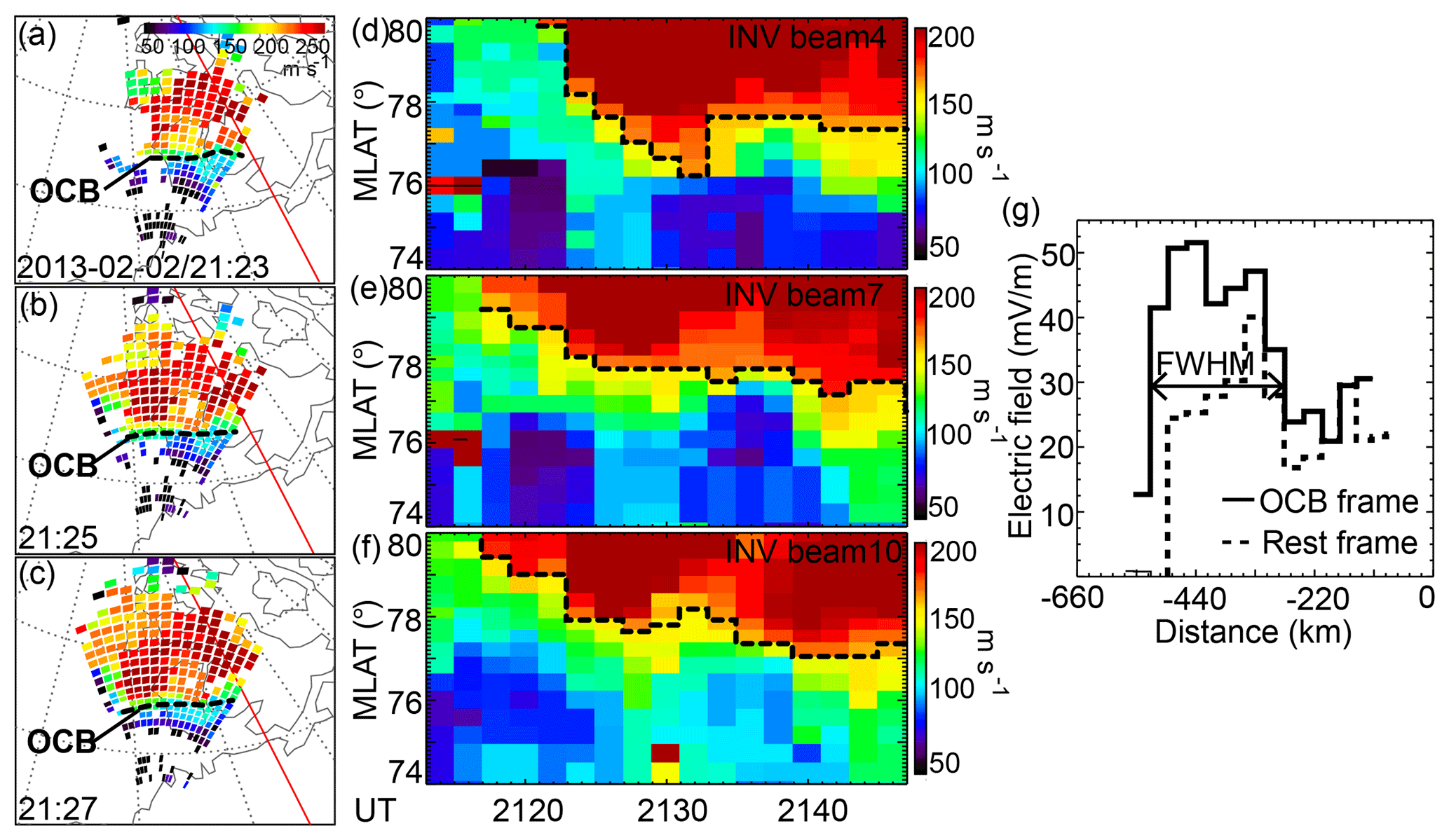
Figure 3 (a–c) Snapshots of spectral width measurements around the space–ground conjunction time and longitude. The open–closed field line boundary is shown as a dashed black line. (d–f) Time series of the spectral width measurements along INV beams 4, 7, and 10 as a function of latitude, from which the motion of the open–closed field line boundary can be derived. (g) The electric field along the open–closed field line boundary in the frame of the boundary (solid) and in the rest frame (dashed) following Pinnock et al. (2003), Freeman et al. (2007), and Chisham et al. (2008). The former is the reconnection electric field.

As shown in Fig. 3g, the profile of the reconnection electric field had a peak in the azimuthal direction with a limited FWHM, and the FWHM is essentially the same as the flow width just poleward of the boundary (the difference being less than the radar spatial resolution). This establishes the relation between our measure of the reconnection jet extent and the extent of reconnection with high reconnection rates. Regions of high reconnection rates are localized, although those of low reconnection rates (> 0 mV m⁻¹) can extend over a much broader region. For example, the western boundary of nonzero reconnection rates was located just at the edge of INV FOV (considering the 15 mV m⁻¹ uncertainty), and the eastern edge extended beyond INV FOV, likely into where the post-noon flow originated. A lower estimate of the extent of nonzero reconnection rates is therefore ∼4 h MLT. It is likely that there were two components of reconnection at different scales: broad and low-rate background reconnection and embedded high-rate reconnection.

To infer the reconnection extent at the magnetopause, we project the flow extent based on the SECS in the ionosphere to the equatorial plane. The result suggests that the reconnection local time extent was ∼2 Re.

3.2 Spatially patchy reconnection active at both satellites

3.2.1 In situ satellite measurements

On 19 April 2015, under a southward IMF (Fig. 4a), THA and THE crossed the magnetopause nearly simultaneously (< 2 min lag) with a 0.5 Re separation in Y (Fig. 4b). They passed from the magnetosheath into the magnetosphere. Both satellites observed jets in the V_L component at the magnetopause (Fig. 5g–p). The jet at THA at ∼18:28:05 UT had a speed of 84 % and an angle within ∼15^∘ of the Walen prediction. The jet at THE at ∼18:26:25 UT had a speed of 95 % and an angle within ∼29^∘ of the Walen prediction. The ion distributions at THA and THE exhibit clear D-shaped distributions. Reconnection thus occurred at both local times.

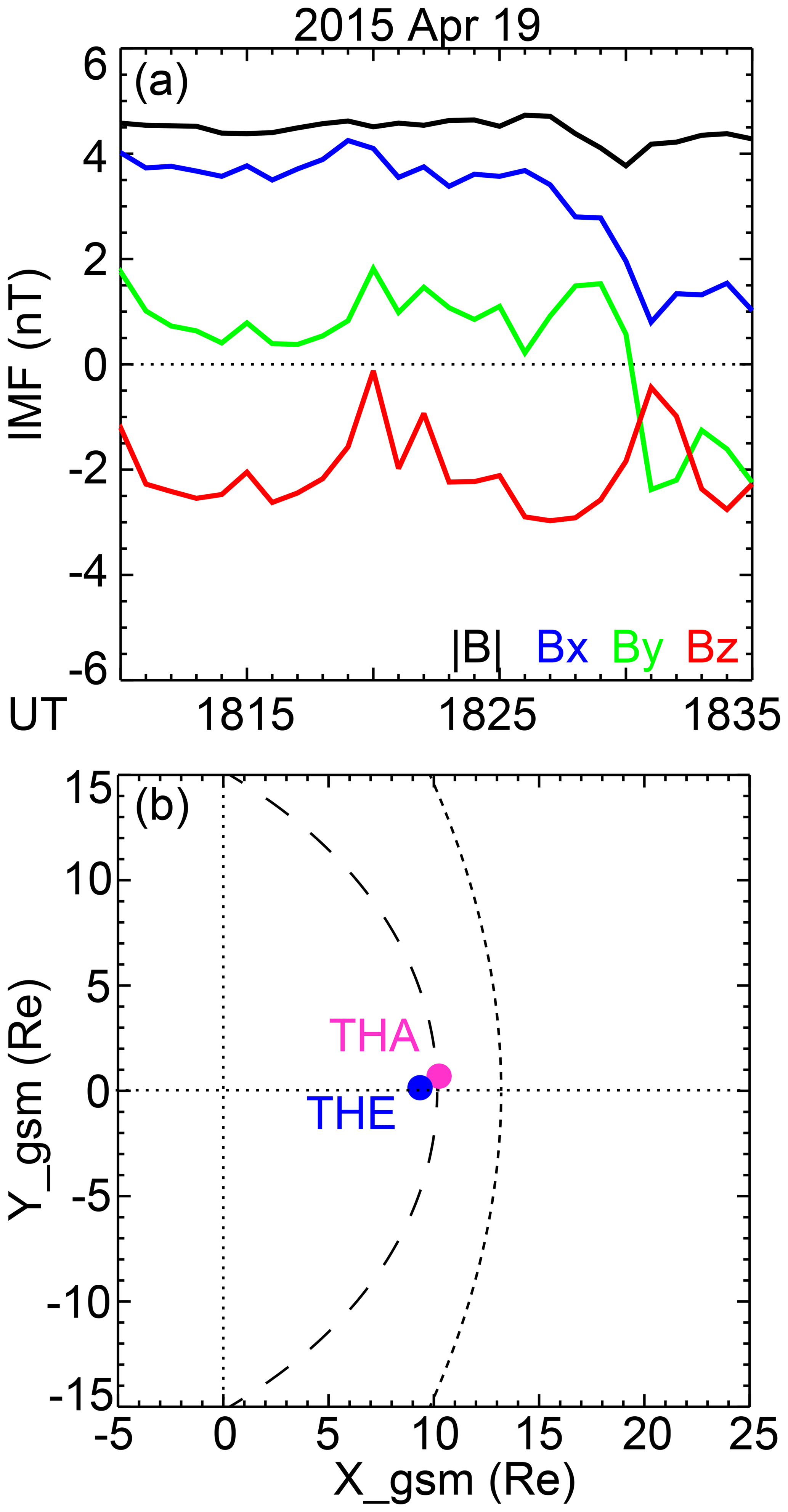
Figure 4 OMNI IMF condition and THEMIS satellite locations on 19 April 2015 in a similar format to Fig. 1.

3.2.2 Ground radar measurements

During the satellite measurements, the radars observed a channel of fast anti-sunward flow around magnetic noon (Fig. 5a–c). The flow crossed the open–closed field line boundary at 77^∘ MLAT and qualifies as an ionospheric signature of magnetopause reconnection jets. The flow direction was nearly parallel to the RKN radar beams, and therefore the RKN LOS measurements in Fig. 5a approximate to the 2-D flow speed. The flow eastern boundary can be identified as where the velocity dropped from red–orange to blue (dashed magenta line). Determining the flow western boundary requires more measurements of the background convection velocity, which is beyond the RKN FOV. But we infer that the western boundary did not extend more than 1.5 h westward beyond the RKN FOV because the PGR and INV echoes there showed weakly poleward and equatorward LOS speeds around the open–closed field line boundary. The CLY radar data further indicated that the anti-sunward flow had started to rotate westward immediately beyond the RKN FOV. This is because the CLY LOS velocities measured between the RKN and INV radar FOVs were larger for more east–west-oriented beams (appearing in yellow) than for more north–south-oriented beams (green). The rotation likely corresponds to the vortex at the flow western boundary as sketched in Oksavik et al. (2004).

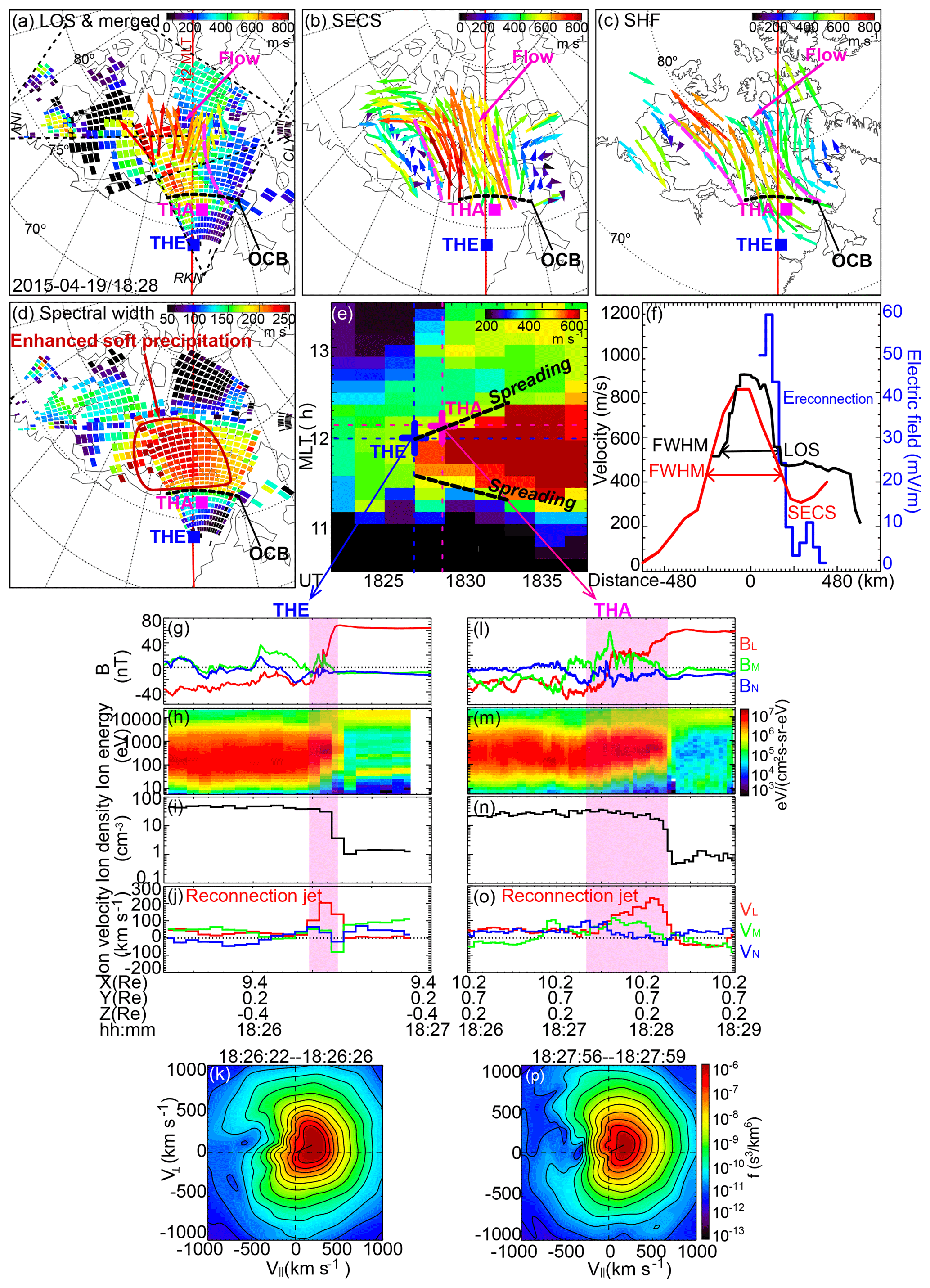
Figure 5 THEMIS and SuperDARN measurements of reconnection bursts on 19 April 2015 in a similar format to Fig. 2. The velocity time evolution in (e) and the velocity profile in (f) are taken along 78^∘ MLAT.

The more precise location of the western boundary can be retrieved from the SECS velocities in Fig. 5b and the SHF velocities in Fig. 5c. The SECS velocities present a flow channel very similar to that in Fig. 5a, while the flow channel in the SHF velocities was more azimuthally aligned than in Fig. 5a–b. It can be seen that across the flow western boundary the flow direction reversed. The equatorward flows are interpreted as the return flow of the poleward flows, as sketched in Southwood (1987) and Oksavik et al. (2004).

The determined flow extent agrees with the extent of the cusp in Fig. 5d. The high spectral widths associated with the cusp were located at the western half of the RKN FOV. They extended westward beyond the RKN FOV into CLY far-range gates, where they dropped from red to green. This is consistent with the inferred location and the extent of the anti-sunward fast flow.

The flow of interest here just emerged from a weak background at the time when the THEMIS satellites crossed the magnetopause (Fig. 5e). This implies that the related reconnection just activated at the studied local time. The flow spread azimuthally until 18:33 UT when it stabilized. We quantify the stabilized flow extent and the reconnection electric field extent (Fig. 5f) in a similar way as Figs. 2f and 3g. The FWHM of the flow is determined to be 432 and 336 km based on the SECS and RKN LOS data, respectively. While the reconnection electric field had data gaps due to limited coverage and backscatter availability at the near-range gate, it implies a western boundary of FWHM consistent with the flow slightly poleward of it. This is also the western boundary of nonzero reconnection rates considering the 15 mV m⁻¹ uncertainty. The eastern boundary extended beyond RKN FOV. The FWHM of the SECS flow profile corresponds to ∼ 4 Re in the equatorial plane.

The fact that the fast anti-sunward flow had a limited azimuthal extent around magnetic noon implies that the corresponding magnetopause reconnection should span a limited local time range around noon. This is consistent with the THEMIS satellite observation in Sect. 3.2.1, showing that reconnection was active at Y=0.7 (THA) and 0.2 Re (THE). Projecting THA and THE locations to the ionosphere reveals that both satellite footprints were located within the flow longitudes. Therefore, the reconnection at the two satellites was part of the same reconnection around the subsolar point of the magnetopause. (The THE footprint was equatorward of THA because the X location of THE was closer to the Earth than THA. The magnetopause was expanding, and it swept across THE and then THA.) The reconnection further extended azimuthally beyond the two satellite locations, reaching a full length of ∼4 Re.

3.3 Spatially continuous and extended reconnection active at both satellites

3.3.1 In situ satellite measurements

On 29 April 2015, under a prolonged and steady southward IMF (Fig. 6a), THA and THE crossed the magnetopause successively with a time separation of ∼30 min. The locations of the crossings were separated by 0.1–0.2 Re in the Y direction (Fig. 6b). The satellites passed from the magnetosphere into the magnetosheath, and the magnetic field data suggest that the satellites crossed the current layer multiple times before completely entering the magnetosheath (Fig. 6i–r). We therefore only display the magnetic field and the plasma velocity in GSM coordinates. Both satellites detected multiple flow jets, all agreeing with the Walen prediction with ΔV^* > 0.5. For example, the jet at 18:49–18:50 UT measured by THA had a speed with 80 % and an angle with 9^∘ of the Walen prediction, and the jet at 19:20–19:22 UT by THE had a speed with 83 % and an angle with 1^∘ of the Walen prediction. The ion distributions at THA and THE exhibit clear D-shaped distributions.

Figure 6 OMNI IMF condition and THEMIS satellite locations on 29 April 2015 in a similar format to Fig. 1.

3.3.2 Ground radar measurements

In the ionosphere, the radars detected a fast anti-sunward flow as an ionospheric signature of the magnetopause reconnection jet (Fig. 7a–c). The flow had a broad azimuthal extent, as delineated by the dashed magenta lines (Fig. 7a). A similar flow distribution is found in the SECS velocities (Fig. 7b) and the SHF velocities (Fig. 7c). The flow propagated into the polar cap as one undivided channel (as opposed to Sect. 3.1.2), implying that it was one flow structure, at least to the resolution the radars can resolve. Corresponding to the broad extent of the flow, the cusp had a broad extent (Fig. 7d). The cusp continuously spanned the INV and RKN FOVs, and its western and eastern edges coincided with the western and eastern boundaries of the flow, supporting our delineation of the flow extent.

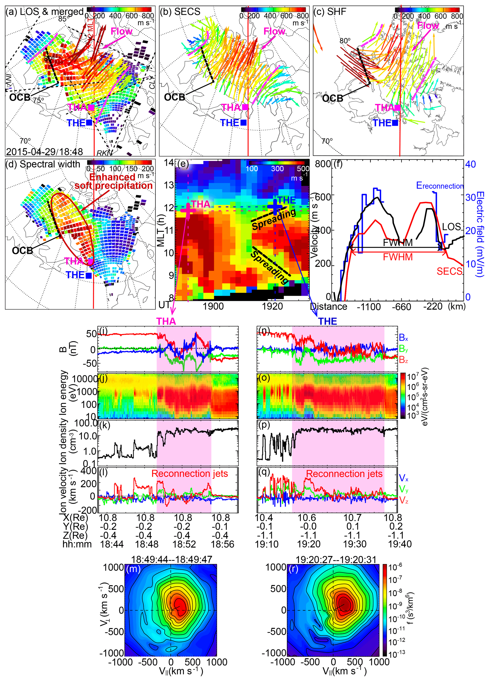
Figure 7 THEMIS and SuperDARN measurements of reconnection bursts on 29 April 2015 in a similar format to Fig. 2. The velocity time evolution in (e) and the velocity profile in (f) are taken along 79^∘ MLAT. The two branches of the LOS velocity profile in (f) are based on INV and RKN LOS data. The magnetic field and plasma velocities measured by spacecraft are displayed in the GSM coordinates.

The wide flow channel in the ionosphere implies that the corresponding magnetopause reconnection jet should be wide in local time. Based on the flow distribution, we infer that much of the reconnection should be located on the prenoon sector, except that the eastern edge can extend across the magnetic noon meridian to the early post-noon sector. This inference is again consistent with the inference from the THA and THE measurements that the reconnection extended at least over the satellite separation ($Y=-\mathrm{0.2}$ (THA) and 0 Re (THE)). Note, however, that the distance between THA and THE only covered < 2 % of the reconnection extent determined from the ionosphere flow. While the satellite configuration and measurements here were similar to those in Sect. 3.2, the extent of reconnection was fundamentally different. This suggests that it is difficult to obtain a reliable estimate of the reconnection extent without the support of 2-D measurements, and satellites alone also cannot differentiate spatially extended reconnection from spatially patchy reconnection.

The flow temporal evolution is shown in Fig. 7e, where the velocities are the northward component of the SECS data. An overall wide flow channel is seen during the time interval of interest here with the eastern and western boundaries located at ∼12.0–12.5 and ∼8.0–8.7 h MLT, respectively. But between the two satellite observations, the flow experienced an interesting variation. The velocity at 9.3–12.0 h MLT dropped by 100–200 m s⁻¹ during 19:02–19:12 UT (red turned orange, yellow, and then green), while the velocity at 8.6–9.3 h MLT did not change substantially. The velocity was enhanced again from 19:12 UT. The enhancement centered at 10.7 h MLT and spread azimuthally towards east and west. The enhancement spread by 0.7 h MLT over 14 min at its eastern end (marked by the dashed black line), suggesting a spreading speed of 275 m s⁻¹. The enhancement spread by 1.2 h MLT at its western end, suggesting a spreading speed of 471 m s⁻¹. It should be noted that all three components of the IMF stayed steady for an extended time (Fig. 8, discussed below in Sect. 4), and thus the evolution of the flow and reconnection was unlikely to be externally driven.

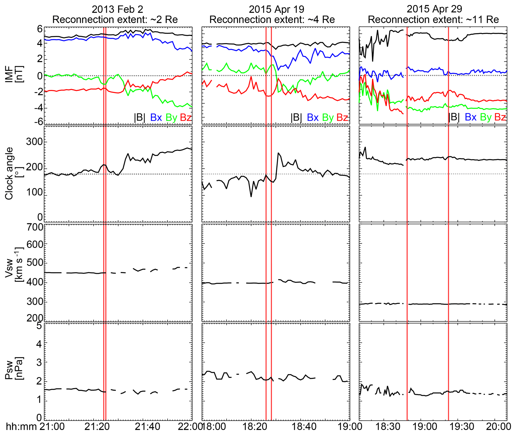
Figure 8 Comparison of the IMF and solar wind driving conditions between the reconnection events on 2 February 2013, 19 April 2015, and 29 April 2015. From top to bottom: IMF in GSM coordinates, IMF clock angle, solar wind speed, and solar wind dynamic pressure. The red vertical lines mark the times of the satellite–ground conjunction.

This sequence of changes gives an important implication that the spatially extended reconnection was a result of the spreading of an initially patchy reconnection. If we map the spreading in the ionosphere to the magnetopause, the spreading occurred bidirectionally and at a speed of 15 and 26 km s⁻¹ in the east and west directions based on field line mapping under the T89 model (the mapping factor was 55). Such an observation is similar to what has recently been reported by Zou et al. (2018), in which the reconnection also spreads bidirectionally at a speed of a few tens of km s⁻¹. However, the spreading in Zou et al. (2018) occurs following a southward turning of the IMF, while the spreading here occurred without IMF variations. The mechanism of spreading is explained either as motion of the current carriers of the reconnecting current sheet or as propagation of the Alfvén waves along the guide field (Huba and Rudakov, 2002; Shay et al., 2003; Lapenta et al., 2006; Nakamura et al., 2012; Jain et al., 2013).

It should be noted that reconnection spreading can be a common process of reconnection that is not limited to extended reconnection. It also occurs for patchy reconnection as seen in Sect. 3.1 and 3.2. The spreading speeds were similar across the three events, but the duration of the spreading process was 2 to 3 times longer in the spatially extended than the spatially patchy reconnection events. For the extended reconnection, the spreading process persisted for 14 min, expanding the extent by 5–6 Re.

Figure 7f quantifies the extent of the flow and reconnection electric field. The FWHM extent was 1320 km based on the SECS data. Despite the presence of data gaps, the LOS measurements suggest a western and eastern boundary consistent with the SECS data. The reconnection electric field had a similar FWHM to the flow, although regions of nonzero reconnection rates again extended beyond the available coverage, indicating an overall extent > 4 h MLT. The extent corresponds to a reconnection extent of ∼11 Re.

4 Discussion

The above events definitely show that the local time extent of magnetopause reconnection can vary from a few to > 10 Re. Here we investigate whether and how the extent may depend on the upstream driving conditions. Figure 8 presents the IMF, the solar wind velocity, and the solar wind pressure taken from the OMNI data for the three events. The red vertical lines mark the times when the reconnection was measured. The three events occurred under similar IMF field strengths (5–6 nT), similar IMF B_z components (−2–3 nT), and similar dynamic pressures (1–2 nPa), implying that the different reconnection extents were unlikely due to these parameters. The solar wind speeds had a slight decreasing trend as the reconnection extent increased. This is different from Milan et al. (2016), who identified a large solar wind speed as the cause of a large reconnection extent. However, Milan et al. (2016) studied reconnection under very strong IMF driving conditions when $\left|B\right|\sim \mathrm{15}$ nT, while our events occurred under a more typical moderate driving ($\left|B\right|\sim \mathrm{5}$–6 nT).

The spatially patchy reconnection events had an IMF B_x of a larger magnitude than the extended reconnection event (4 vs. 0 nT). The spatially patchy reconnection events also had an IMF B_y component of a smaller magnitude (2 vs. 5 nT, and therefore a clock angle closer to 180^∘), and with more variability on timescales of tens of minutes, than the extended reconnection event. The IMF B_x and B_y components are known to modify the magnetic shear across the magnetopause and to affect the occurrence location of reconnection. Studies have found that at the dayside low-latitude magnetopause small |B_y|∕|B_z| relates to antiparallel and large |B_y|∕|B_z| to component reconnection (Coleman et al., 2001; Chisham et al., 2002; Trattner et al., 2007). Large $\left|B_x|/|B\right|$, i.e., cone angle, also favors the formation of high-speed magnetosheath jets (Archer and Horbury, 2013; Plaschke et al., 2013) of a few Re in scale size, resulting in a turbulent magnetosheath environment for reconnection to occur (Coleman and Freeman, 2005). The steady IMF condition may allow reconnection to spread across local times unperturbedly, eventually reaching a wide extent. Thus our preliminary analysis suggests that the reconnection extent may depend on the IMF orientation and steadiness, although whether and how they influence the extent needs to be further explored.

5 Summary

We carefully investigate the local time extent of magnetopause reconnection by comparing measurements of reconnection jets by two THEMIS satellites and three ground radars. When reconnection jets are only observed at one of the two satellite locations, only the ionosphere conjugate to this spacecraft shows a channel of fast anti-sunward flow. When reconnection jets are observed at both spacecraft and the spacecraft are separated by < 1 Re, the ionosphere conjugate to both spacecraft shows a channel of fast anti-sunward flow. The fact that the satellite locations are mapped to the same flow channel suggests that the reconnection is continuous between the two satellites and that it is appropriate to take the satellite separation as a lower limit estimate of the reconnection extent. Whether reconnection can still be regarded as continuous when the satellites are separated by a few or > 10 Re is questionable and needs to be examined using conjunctions with a larger satellite separation than what has been presented here.

The reconnection extent is measured as the FWHM of the ionospheric flow. In the three conjunction events, the flows have FWHM of 200, 432, and 1320 km in the ionosphere, which corresponds to ∼2, 4, and 11 Re at the magnetopause (under the T89 model) in the local time direction. The flow extent is confirmed to be related to reconnection with a high reconnection electric field. The result provides strong observational evidence that magnetopause reconnection can occur over a wide range of extents, from spatially patchy (a few Re) to spatially continuous and extended (> 10 Re). Interestingly, the extended reconnection is seen to initiate from a patchy reconnection, whereby the reconnection grows by spreading across local time. The speed of spreading is 41 km s⁻¹, summing the westward and eastward spreading motion, and the spreading process persists for 14 min, broadening the extent by 5–6 Re.

Based on the three events studied in this paper, the reconnection extent may be affected by the IMF orientation and steadiness, although the mechanism is not clearly known. For the observed modest solar wind driving conditions, spatially extended reconnection is suggested to occur under a smaller IMF B_x component and a larger and steadier IMF B_y component than spatially patchy reconnection. The IMF strength, the B_z component, and the solar wind velocity and pressure are about the same for the extended and the patchy reconnection. This finding, however, could be limited by the number of events under analysis, and further study is needed to achieve an understanding of how solar wind controls reconnection extent. Reconnection can vary with time, even under steady IMF driving conditions.