the Creative Commons Attribution 4.0 License.
the Creative Commons Attribution 4.0 License.
 | 28 Mar 2019
Solar-eclipse-induced perturbations at mid-latitude during the 21 August 2017 event
Bolarinwa J. Adekoya
Babatunde O. Adebesin
Timothy W. David
Stephen O. Ikubanni
Shola J. Adebiyi
Olawale S. Bolaji
Victor U. Chukwuma
A study of the response of some ionospheric parameters and their relationship in describing the behaviour of ionospheric mechanisms during the solar eclipse of 21 August 2017 is presented. Mid-latitude stations located along the eclipse path and with data available from the Global Ionospheric radio Observatory (GIRO) database were selected. The percentage of obscuration at these stations ranges between 63 % and 100 %. A decrease in electron density during the eclipse is attributed to a reduction in solar radiation and natural gas heating. The maximum magnitude of the eclipse consistently coincided with a hmF2 increase and with a lagged maximum decrease in NmF2 at the stations investigated. The results revealed that the horizontal neutral wind flow is as a consequence of the changes in the thermospheric and diffusion processes. The unusual increase and decrease in the shape and thickness parameters during the eclipse period relative to the control days points to the perturbation caused by the solar eclipse. The relationships of the bottomside ionosphere and the F2 layer parameters with respect to the scale height are shown in the present work as viable parameters for probing the topside ionosphere during the eclipse. Furthermore, this study shows that in addition to traditional ways of analysing the thermospheric composition and neutral wind flow, proper relation of standardized NmF2 and hmF2 can be conveniently used to describe the mechanisms.
- Article
(6423 KB) - Full-text XML
- BibTeX
- EndNote


A solar eclipse provides opportunity to study the causes of drastic changes in the atmosphere arising from reduction in solar radiation and plasma flux. The atmosphere responded to these changes by modifying the electrodynamic processes and ionization supply of its species to the nighttime-like characteristics during the daytime. Different physical mechanisms (e.g. neutral wind, thermospheric composition, diffusion process) that explain the distribution of plasma at the different ionospheric layers are well established. However, these mechanisms do compete with themselves in explaining the ionosphere, especially the topside ionosphere (see Gulyaeva, 2011).
At mid-latitudes, the effect of diffusion processes and its relationship with the thermospheric compositions has been extensively studied during episodes of a solar eclipse (Müller-Wodarg et al., 1998; Jakowski et al., 2008; Le et al., 2009; Wang et al., 2010; Chuo, 2013). At equatorial and low-latitude regions, the E×B plasma drift had been used to explain the circumstances of a solar eclipse on transport processes (Adeniyi et al., 2007; Adekoya et al., 2015). Recently, attention has been drawn to the study of the topside ionosphere during an eclipse for improved prediction and modelling (Huba and Drob, 2017; Chrniak and Zakharenkova, 2018). Reinisch et al. (2018) compared the modelled and measured studies of electron densities at the altitude range of about 150–400 km during the eclipse. They found that at a lower altitude (at about 150 km) the modelled and the measured data agreed well with the changes in the altitude profile of electron density compared to those at higher altitudes. The authors, however, posited that it would be improved if the model NmF2 peak falls more slowly to better match the data. Consequently, the present study investigates the effects of the solar eclipse of 21 August 2017 on the constituents of the ionosphere at mid-latitudes using some ionosonde data (bottomside parameters, scale height H estimated from the fitted α-Chapman layer) which have not been given much attention in previous works, especially in analysing solar eclipse effect. Using these parameters to analyse the circumstances of the solar eclipse at the topside ionosphere and its plasma distribution mechanisms makes this paper significantly different from previous studies. Thus, we intend to analyse the ionospheric parameters that control the distribution of plasma at the topside and bottomside layers of the F2 region. To shed light on these analysis, Sect. 2 highlights the data source, methodology and path of the eclipse. The results and discussion were presented in Sect. 3, while Sect. 4 presents the summary and concluding remark of the result.
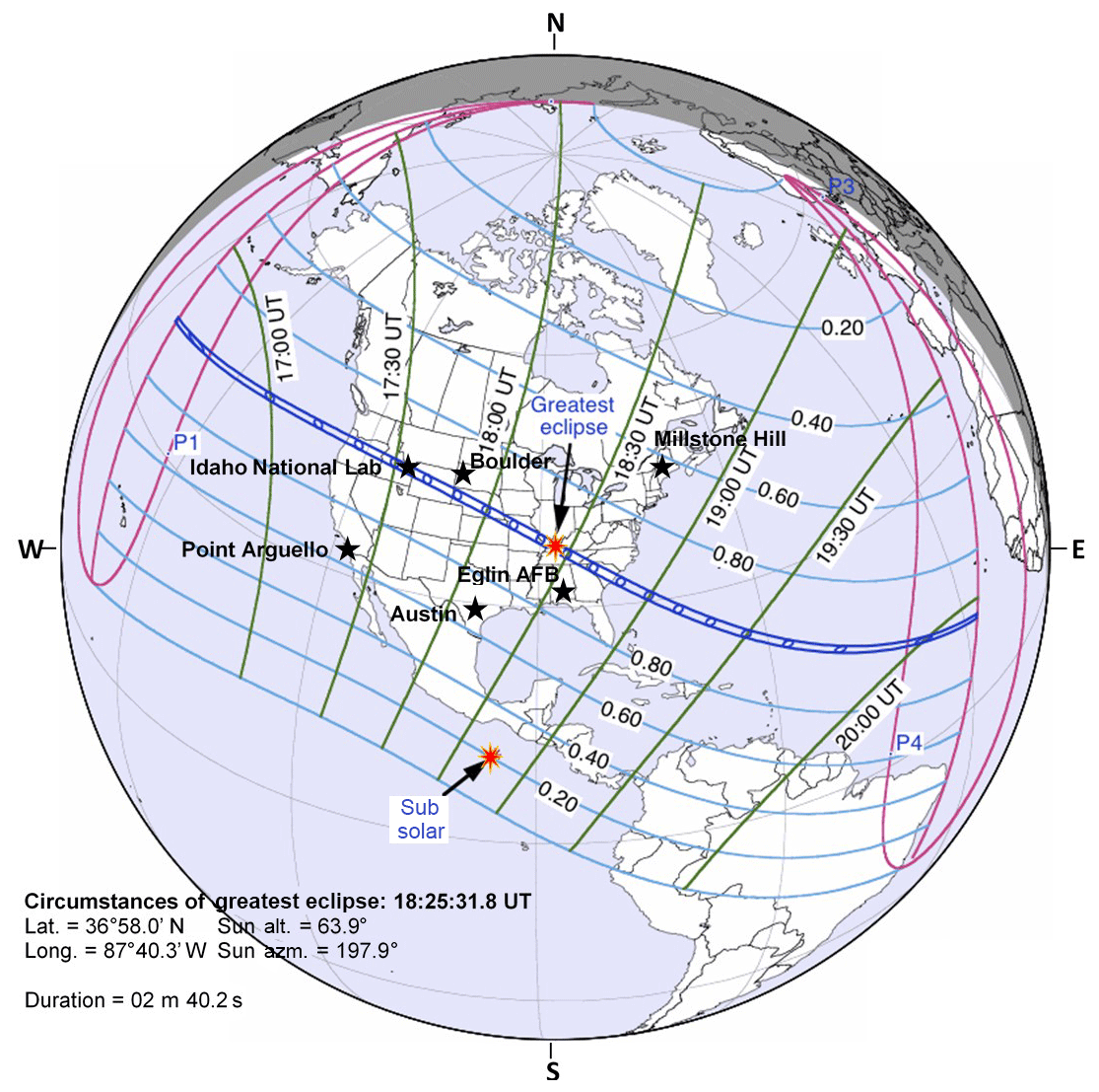
Figure 1The orthographic map showing the coverage area and circumstances of the solar eclipse, and the observatory stations of the total solar eclipse event of 21 August 2017 . The thick blue line region of represents the path of the maximum magnitude of the eclipse and the pale blue lines mark the region of where the partial eclipse is experienced, with the magnitude of partiality.
With regards to the eclipse of 21 August 2017, the totality of the eclipse is visible from within a narrow corridor that traverses the United States of America. However, in the surrounding areas, which include all of mainland United States and Canada, the eclipse was partial. From the footprint of the Moon's shadow as seen from some locations, the eclipse started from around 17:00 UT and ended around 20:00 UT. Figure 1 shows the coverage area and circumstances of the solar eclipse in detail. More details of its path can be seen via NASA (Total solar eclipse of 21 August 2017; https://eclipse.gsfc.nasa.gov/, last access: 25 March 2019). The details on the local circumstances of the eclipse and the time of the first, middle and last contact of the eclipse over the ionosphere of the investigated stations was highlighted in Table 1. More details on the total solar eclipse event and its partiality, the circumstances surrounding its progression and its magnitude of obscuration can be obtained at http://xjubier.free.fr/en/index_en.html (last access: 25 March 2019). The path of the eclipse informed the choice of stations. The ionospheric data used for this study for the selected mid-latitude stations were obtained from the Global Ionospheric Radio Observatory (GIRO) networks (http://giro.uml.edu/, last access: 25 March 2019) (Reinisch and Galkin, 2011) and manually validated. The calculated daily average of summation Kp, Ap and solar flux indices was obtained from the National Space Science Data Centre's (NSSDC's) OMNI database https://omniweb.gsfc.nasa.gov/ (last access: 25 March 2019).
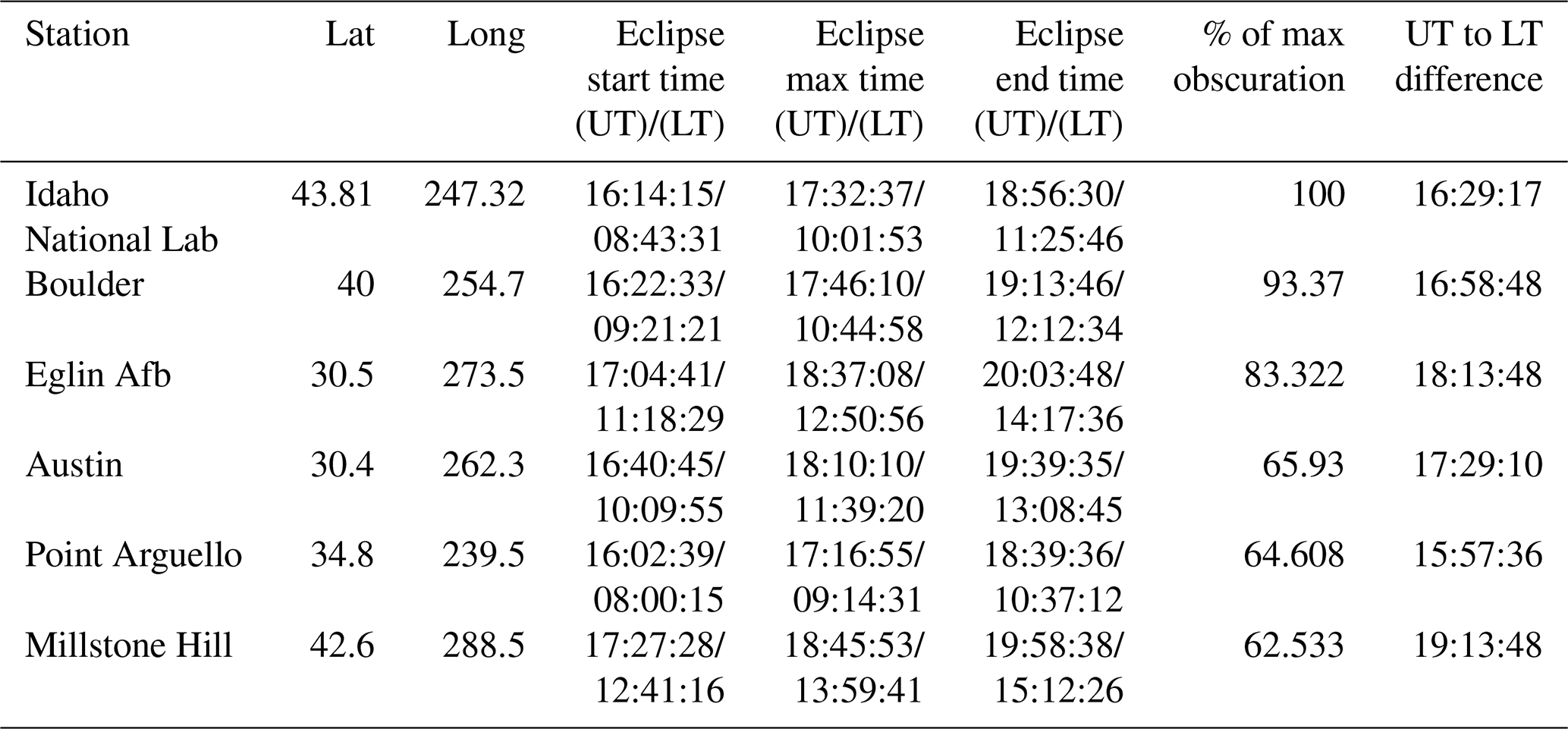
Table 1List of ionosonde stations, geographic coordinates, eclipse progression times (universal time/local time) and percentages of maximum obscuration.
NmF2 values for both the eclipse and control days were obtained from their corresponding critical frequencies (foF2) using the following expression: NmF2 = ((foF2)2∕80.5)e m−3. The control day value is the average value of the two days before and after the eclipse day (i.e. 6, 12, 24 and 27). These reference days were chosen such that they have similar geomagnetic, interplanetary and solar properties with the eclipse day. The daily average values of control days, eclipse day interplanetary indexes (Ap and Kp) and the solar flux unit (sfu) index (F10.7) range from 8 to 12 nT for the Ap index, 2 to 3 for the Kp index and 75.6 to 89.1 sfu (1 sfu = 10−22 Wm−2 Hz−1) for F10.7, indicating that the geomagnetic and solar activities of these days are unsettled (see Adekoya et al., 2015, for classification of geomagnetic activity). The typical behaviour of the NmF2 and hmF2 on the eclipse day (i.e. NmF2e and hmF2e) was compared with that of the control day (NmF2c and hmF2c) to observe the changes brought by the short period of loss of photoionization in the ionosphere. This will measure the direct consequence of the solar radiation disruption (due to the eclipse) on the ionospheric chemical, transport and thermal processes in the F2 layer. The ionized layer depends majorly on three parameters, viz. NmF2, hmF2 and the plasma scale height (Hm).
The GIRO provides access to autoscaled values of ionospheric parameters generated by the automatic real-time ionogram scaler with true height (ARTIST) algorithm, which is inherent in the UMLCAR-SAO Explorer (Reinisch and Huang, 1983; Galkin et al., 2008; Reinisch and Galkin, 2011), and facilitates the derivation of bottomside profiles. From the ULMCAR-SAO Explorer, the manually scaled ionogram with high accuracy are calculated from the standard true-height inversion program (Reinisch and Huang, 1983; Huang and Reinisch, 1996). The parameters obtained include the critical frequency (foF2, Hz), its height (hmF2, km) of the F layer, and the shape (B1) and thickness (B0) parameters. Likewise, the scale height (Hm) of the F2 layer is obtained from the bottomside. It is estimated from the fitted α-Chapman function with a variable scale height, H(h), to the measured bottomside profile N(h), which is then determined as the Chapman scale height at hmF2 (i.e. H(h> hmF2) ≈Hm (hmF2)) (Huang and Renisch, 2001; Reinisch and Huang, 2001; Reinisch et al., 2004). The topside profile is then related to the scale height at the layer, from the bottomside profile, represented with α-Chapman function (Reinisch and Huang, 2001). This is because the Chapman function described the electron density profile, N(h), aptly. Also, Hm provides a linkage between the bottomside ionosphere and the topside profiles of the F region (Liu et al., 2007). Therefore, Hm describes the constituents of the ionospheric plasma, which decreases with increasing altitude. The fitting formulas of α-Chapman function are provided in Eq. (1) below.
where all the parameters have their previously defined meaning.
However, Xu et al. (2013) and Gulyaeva (2011) related ionospheric F2-layer scale height, H, to the topside base scale height, Hsc, given by Hsc = hsc − hmF2 ≈ 3 × Hm). In their work, hsc is the height at which the electron density of the F2-layer falls by a factor of an exponent, at an upper limit of 400 km altitude (i.e. NmF2 ∕e) (see Xu et al., 2013), that is, the region where electron density profile gradient is relatively low. Gulyaeva (2011) showed theoretically that a Hsc increase over Hm by a factor of approximately 3 is a consequence of the Ne ∕ NmF2 ratio (Ne: plasma density), which corresponds to Hm in the Chapman layer. At altitudes very close to hmF2, the ratio equals 0.832, while it is 0.368 at altitudes beyond the hmF2. Therefore, we adopted the definition of Gulyaeva (2011) for the topside base scale height as the region of the ionosphere between the F2 peak and 400 km altitude. Summarily, the topside-based scale height ionosphere here is defined as the region between the F2 peak and hsc or 3Hm. It is thus evident that Hm is a key and essential parameter in the continuity equation for deriving the production rate at different altitudes, a pointer to the F2 topside electron profiler, as well as a good parameter for evaluating the transport term (Yonezawa, 1966; Huang and Reinisch, 2001; Reinisch and Huang, 2001; Belehaki et al., 2006; Reinisch et al., 2004). Consequently, the parameter Hm can be used as a proxy for observation relating to the topmost side electron density profile. Furthermore, the division of the topside and the bottomside ionosphere may be related to the difference in the effective physical mechanisms in the regions. Hence, the bottomside parameters B1 and B0 of the ionosphere, as presented in this work, helped in examining the perturbation of the solar eclipse in the bottomside ionospheric F2 layer.
This section presents the temporal evolution of the maximum electron density (NmF2), and its corresponding height (hmF2) over the ionosphere at the selected mid-latitude stations along the path of the solar eclipse of 21 August 2017. The control day variation relative to the eclipse day is also presented. Figure 2 presents the variation in maximum electron density and the corresponding peak height, during both the eclipse and control days. Figure 3 depicts the variation in scale height and the bottomside parameters (B0 and B1) due to the eclipse by superposing plots for both the eclipse and control days. Analysis of these parameters during an eclipse event may help in the modelling of the ionospheric profiles (the topside and bottomside electron density distribution profile) during the short nighttime-like period of the day.
Figure 2a presents the NmF2 and hmF2 variations during the eclipse event and the control day over the Idaho National Lab, with an obscuration magnitude of 100 % around the daytime period. The effect of the disruption of solar radiation was evident as the NmF2 started decreasing at the first contact of the eclipse compared to an incessant increase on the control day in Fig. 2ai. The start time or first contact (08:43:31 LT), the maximum magnitude period (10:01:53 LT) and the end time or the last contact (11:25:46 LT) of the eclipse are marked with the vertical lines S, M and E respectively. The decrement in NmF2 during the eclipse phase was due to reduction in the ionization. This reduction caused changes in the photochemical and transport process of the atmosphere during the daytime, thus exhibiting nighttime characteristics. It should be noted that the maximum decrease in NmF2 did not coincide with the maximum magnitude of the eclipse obscuration, but rather with a time lag of few minutes, i.e. at 10:30 LT. This lag period fell within the relaxation period over the Idaho ionosphere, with NmF2 and hmF2 simultaneously attaining their peak magnitudes of 1.67 e m−3 and ∼239 km. Hence, the ionosphere returned to its pre-eclipse state. Contrary to the decrease in the NmF2 amplitude at the recovery phase of the eclipse, hmF2 increases, attains 239 km peak around 10:30 LT and then decreases, depicting the eclipse-caused morphology.
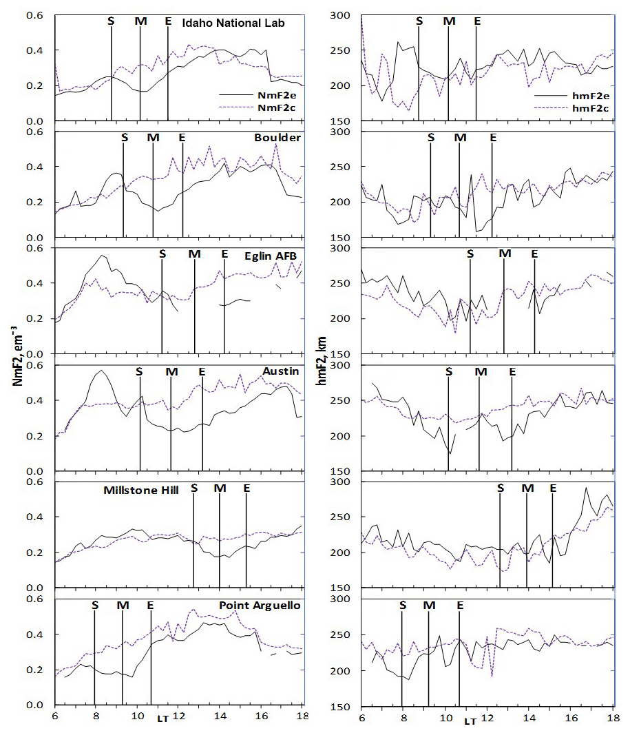
Figure 2Ionospheric NmF2 and hmF2 variations during the eclipse day (black continuous line) and the control day (dash blue line) were presented to delineate the effect of the solar eclipse of 21 August 2017 on the ionosphere. The three vertical lines represents the different phases of the eclipse (S – start time of the initial phase, M – the period of the maximum magnitude of the eclipse, and E – the end time of the recovery phase or the last contact of the eclipse progression). The local time of the respective eclipse contact points for each station are given in Table 1.
The ionosphere over Boulder, Eglin AFB, Austin, Millstone Hill and Point Arguello did not show any contrary variation to that observed over Idaho during the eclipse event. The decrease and increase in NmF2 and hmF2 after the maximum magnitude are simultaneous. The only exception was that the local time at which each station observed the effects was different. Their obscuration percentage ranged from 62.5 % to 93.37 %. This did not cause any significant change in the way they responded to the reduction in solar heating. The ionosphere over Boulder experienced the totality of the eclipse with 93.37 % magnitude, which is next to Idaho (100 %) in obscuration, and the hmF2 was observed to increase few minutes after the maximum magnitude of the obscuration. This behaviour is typical for other stations at the eclipse window, but the time of NmF2 minimum decrease did not always coincide with the hmF2 enhancement after the maximum obscuration. These observations posit that the minimum rate of electron production does not necessarily translate to the peak electron density of the molecular gases formed. This is because the electron concentration depends on the loss rate by dissociative recombination, too.
At mid-latitudes, the ionospheric F2 plasma distribution is controlled by diffusion processes (Rishbeth, 1968). There are two basic mechanisms that define the diffusion process during an eclipse: first is the coolness brought by the partial removal of photoionization (Müller-Wodarg et al., 1998), which is believed to instigates the downward diffusion process, and second is the atmospheric expansion due to the gradual increase in the temperature after the totality. The downward diffusion process was related to the increase in the molecular gas (N2) concentration during the cooling process. However, the aftermath of the coolness was related to the upward diffusion process. These mechanisms were proxy to the electron density distribution during the eclipse window. Our analysis suggests that the observed decrease in NmF2 is due to the downward diffusion flux of the plasma while the increase that followed is by upward diffusion (e.g. Le et al., 2009; Adekoya and Chukwuma, 2016). Several works on eclipse (Müller-Wodarg et al., 1998; Grigorenko et al., 2008; Adekoya and Chukwuma, 2016; Hoque et al., 2016) have shown that it was not just the electron density that is being affected during an eclipse window, but the thermospheric wind as well, since the thermospheric wind emanating from the ratio of gas species is related to the variation in electron density. It has been observed that the increase in the mean molecular gas of thermospheric composition decreases the electron density and vice versa. Le et al. (2010) related the valley of electron density distribution during the eclipse phases to the contraction/compression and expansion of the atmosphere brought by the decrease and increase in temperature. Chukwuma and Adekoya (2016) attributed the decrease in the electron temperature to the downward vertical transport process and the decrease in the cooling process to the upward vertical transport process.
Figure 3 describes the variation in Hm, B1 and B0 in three columns respectively for all the stations. Looking at the Hm plots, one can see that there was a defined morphological representation of Hm at the eclipse window. From the first contact of the eclipse, there was an incessant increase in peak variation that maximized some minutes after the maximum contact of the eclipse, i.e. about 15–45 min later. Following the peak magnitude after the maximum contact of the eclipse, the Hm sharply decreases, reaching the minimum peak before its rather increase throughout the remaining period of the eclipse second phase. It was further observed that the minimum decrease in NmF2 amplitude corresponds to an increase in Hm at all stations, implying the upward lifting of the topside electron to the region of higher altitude at the eclipse window. Hence, the scale height variation highlights the decrease in electron production and the vertical distance through which the pressure gradient falls at the topside during the eclipse activity. The observation illustrates the mutual relationship between the NmF2 and Hm, which may aid in extrapolating the topside ionospheric profile (Gulyaeva, 2011). In essence, scale height changes observed during the eclipse window can be used to explain the pressure gradient, electron density distribution and transport processes. In this sense, the diffusion coefficients are expressed as a ratio of determinants (determinant here refers to the concentration of species ([O] and [N2]), with the size of the determinants depending upon both the number of species in the gas mixture and the level of approximation. Therefore, the increase (decrease) in the scale height can be used as a proxy for the downward (upward) diffusion process at the topside ionosphere. Consequently, the thermospheric wind, which causes plasma distribution in the topside ionosphere, is induced by solar radiation. Moreover, the significant changes observed in the scale height variation during the eclipse window also indicated that transport processes are affected as they are temperature dependent. Therefore, changes in the thermospheric compositions due to the solar eclipse at the topside layer will affect the density profiles of the ionosphere.
It is noteworthy that the increase (decrease) in the scale height decreases (increases) the electron density during the eclipse window. The sensitivity of electron density to temperature at the topside directly affects the electron density profile (e.g. Wang et al., 2010), as cooling due to the decrease in temperature results in the decrease in the electron density via reduced ionization. This indicates that the decrease (increase) in electron temperature at the topside ionosphere causes the increase (decrease) in the scale height, which is related to the diffusion and transport processes and subsequently affect the pressure gradient of the plasma. From plots of Hm (Fig. 3) and NmF2 (Fig. 2), it was observed that the minimum decrease in NmF2 corresponded with the peak increase in scale height. This implies that the topside ionosphere is more sensitive (than the bottomside) to any changes in the solar radiation. Thus, the pressure gradients can be analysed in terms of either the scale height or electron density during the solar eclipse.
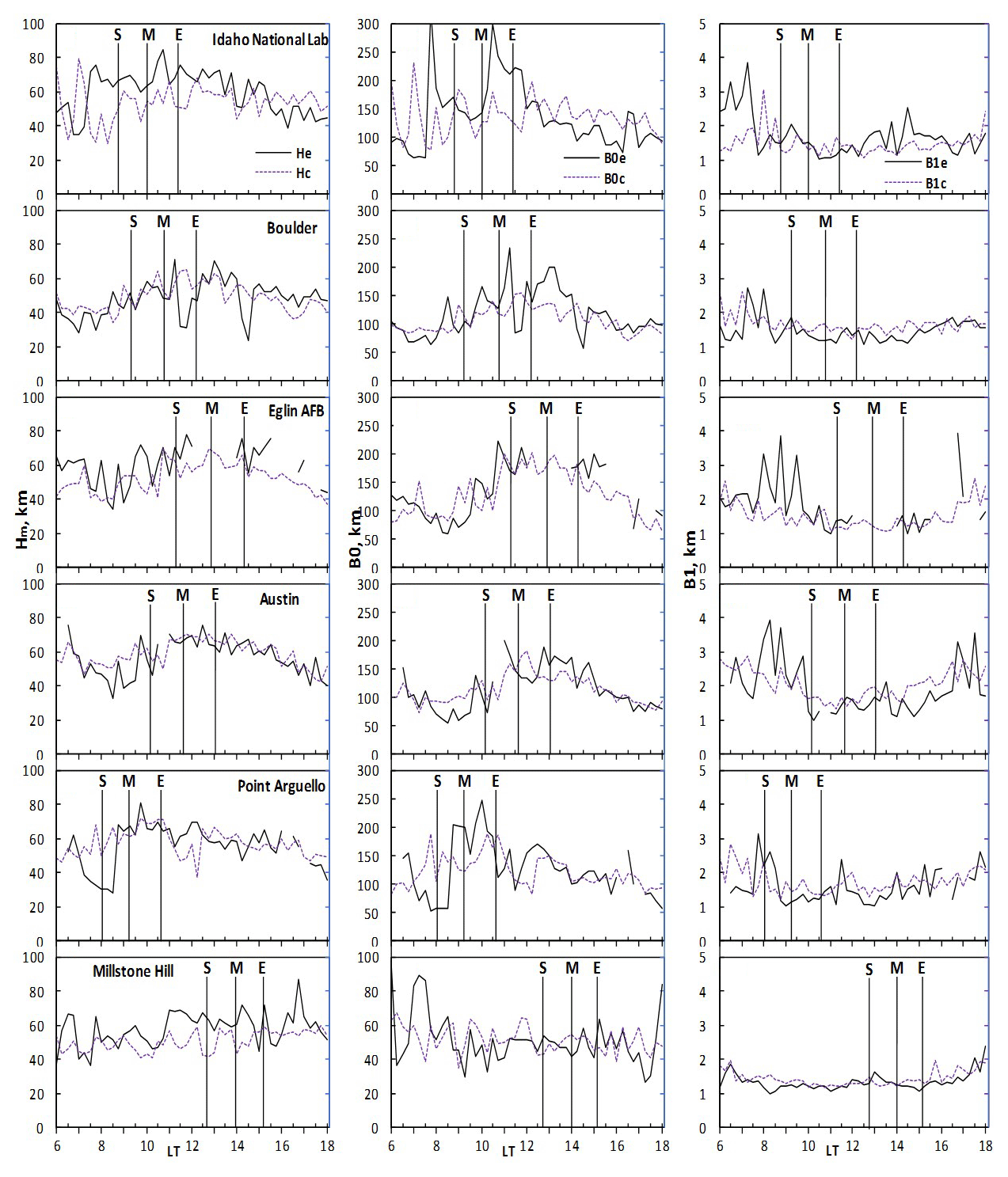
Figure 3The local time variation in the ionospheric scale height and the bottomside (B0 and B1). The other features are the same as in Fig. 2.
From column 2 and 3 of Fig. 3, we observed that the measured shape (B1) and thickness (B0) parameters of the ionosphere over these stations exhibit significant variations during the eclipse event. B1 responded with a decrease at the first contact of the eclipse compared to the control day. This decrease was gradual throughout the eclipse window and followed the variation in solar ionizing radiation. However, the B0 variation differs from that of the B1 observation. The B0 increases from the first contact and reached the maximum peak a few minutes after the maximum obscuration magnitude, which coincided with the minimum decrease in B0. Generally, the pattern of the day-to-day variation in the bottomside parameters was the average morphology, but the increase in the B0 and the decrease in the B1 parameters during the eclipse period compared to the control day was a notable one and can be related to the perturbation caused by the solar eclipse. During the eclipse, the solar radiation was lost; trapped atomic ions (O+) were converted into molecular ions (NO+ and O) by charge transfer, owing to the sufficient concentration of molecular gasses (N2 and O2) (Rishbeth, 1988). The height of the ionospheric slab indeed increased with reduced width, which is attributable to compression due to loss of solar heating.
The behaviour of the ionosphere during the solar eclipse can be explained with any of the components that constitute the topside and the bottomside ionosphere and can be looked at from the angle of the percentage of concentration of the components. In this regard, the deviation percentage of NmF2 (δNmF2) and hmF2 (δhmF2) during the eclipse day away from the control day were plotted in Fig. 4. This is done to describe the contribution of the thermospheric wind and compositions. Although observing the variation in NmF2 and hmF2 alone can be used for observing the changes in the behaviour of the thermospheric compositions and wind flow, if properly analysed, it is more convenient to describe these mechanisms by standardizing the original variables used during the event. The normalization effort (with the use of δNmF2 and δhmF2) presents the original variation in NmF2 and hmF2 in directions which maximize the variance. Consequently, the result can be used for analyses of any mechanisms that drive the ionospheric plasma, if properly related.

Figure 4Variation in the deviation percentage of NmF2 (δNmF2) and hmF2 (δhmF2) magnitudes for observing the changes in the behaviour of the thermospheric composition and wind flow related to the loss rate during the eclipse phase. The three vertical dashed lines marked the eclipse start time, the time of maximum obscuration and the last contact time of the eclipse (i.e. eclipse phase). Table 1 highlights the local time contact point of the eclipse corresponding the international standard time (IST) eclipse progression. The direction of wind was identified using the δNmF2 colour legend. The negative values represent the westward wind direction and the positive values represent the eastward wind.
The deviation percentage in Fig. 4 was defined as the ratio of ((NmF2e − NmF2c) ∕ NmF2c) × 100. The same relation is defined for the hmF2 parameter. As pointed out earlier, during the eclipse period, neutral composition becomes the dominant chemical process arising from diffusion activities. The increase in the neutral composition leads to the increase in the molecular gas concentration and competes with the diffusion process. Hence the deviation percentage discusses the neutral composition changes and delineate how these changes may affect the electron densities as well as its profiles in the atmosphere during the eclipse. The respective maximum and minimum peak response of the deviation percentage is attributed to the enhancement and depletion of δNmF2. One can sees from the plots that the deviation percentage started increasing at the first contact of the eclipse (the first dashed vertical line) and reached the maximum, appearing a few minutes after the maximum magnitude of the eclipse (the second dashed vertical line). This behaviour is similar to the conditions of the neutral compositions during the eclipse event reported by Müller-Wodarg et al. (1998).
Another important process observed in this study is the neutral wind flow effect. To identify the direction of the wind, the δNmF2 colour legend in the contour plots was used in Fig. 4. The negative values represent a westward wind contribution and the positive values is for the eastward wind. Looking at the marked eclipse region in the figure, it was revealed that the δNmF2 started decreasing from the first contact of the eclipse, maximized a few minutes after the maximum contact mark and decreased thereafter. It has been established that at daytime, the peak height of the plasma will be reduced due to lost in recombination. At nighttime, equatorward neutral wind drives the F2-layer plasma to higher altitudes where the recombination rate is slower. The ionospheric processes during the solar eclipse are said to represent a partial nighttime–sunset ionospheric process (Adekoya et al., 2015; Adekoya and Chukwuma, 2016). Thus, the F2 plasma behaviour at the eclipse window is induced by the equatorward neutral wind flow. The neutral wind acts jointly with the plasma flows from the topside ionosphere, resulting in F2 region plasma density variation. Therefore, the westward (eastward) neutral wind flow is related to the depletion (enhancement) in the deviation, which was clearly shown in the marked eclipse region of the figure. The plots in Fig. 3 establish the ionospheric dynamics of diffusion processes, neutral compositions and the flow of neutral wind caused by the eclipse perturbation, which can invariably reduce the effectiveness and reliability of radio wave propagation.

Figure 5Linear relationship of H versus hmF2 and H versus B0 during the progression phase of the eclipse of 21 August 2017.
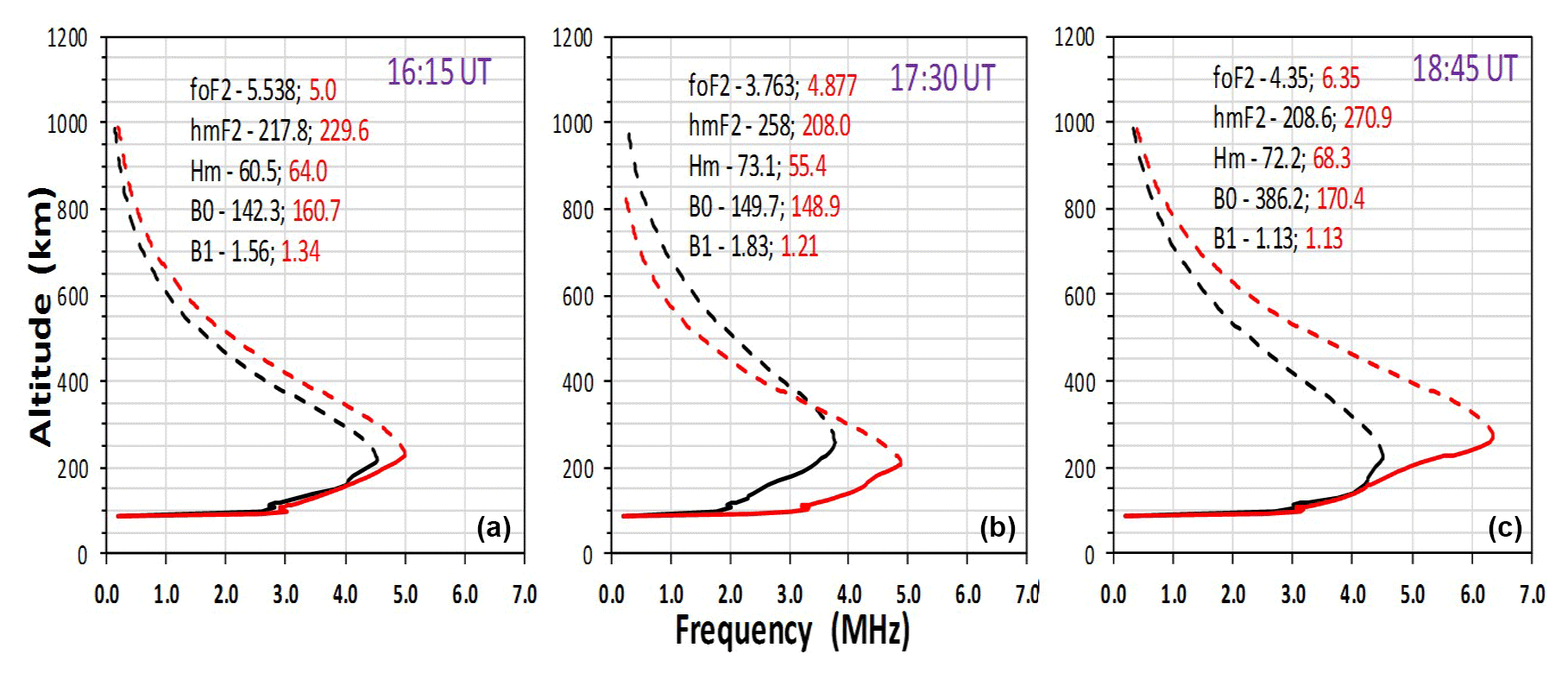
Figure 6Example of the ionospheric profile at the eclipse window of Idaho National Lab showing the bottomside profile (continuous line) and the modelled topside profile shown as a dashed line. The maximum point of the continuous line is the point in which the peak value of the measured foF2 and hmF2 are obtained. The respective measured values foF2 and hmF2 and the corresponding B1, B0, and Hm parameters values are provided in the plot. The black curve represents the profile for the eclipse day (21 August) and the red curve is for the selected reference day, 27 August. Panel (a) shows the profile during the first contact of the eclipse, and (b) and (c) show profiles for the maximum contact and the last contact of the eclipse respectively.
Relative to the mutual relationship between the topside and bottomside ionosphere, we considered the linear correlation coefficient (R) of Hm versus hmF2 and H versus B0 during the eclipse window. In Fig. 5, R ranges from 0.80 to 0.90 for the Hm∕ hmF2 relationship and from 0.57 to 0.89 for the Hm∕ B0 connection. This good linear agreement revealed the dependence of hmF2 and B0 on the scale height. Apart from revealing the dependence between the parameters, the relationship may also provide a convenient way to model the topside profile from the knowledge of the bottomside parameter, B0, during the eclipse period. Further, Fig. 6 illustrates the relationship between the bottomside (continuous line) and the topside (dashed line) ionosphere over Idaho National Lab during the solar eclipse compared to the non-eclipse period. Panel (a) shows the ionospheric profile during the first contact of the eclipse, and panels (b) and (c) show profiles during the maximum contact and last contact of the eclipse respectively. The black curve represents the profile for the eclipse day (21 August) and the red curve is for the selected reference day, 27 August. It is clear from the plots that the ionospheric profiles vary with the solar ionizing radiation at the eclipse window and show the suitability of using the bottomside F-region for probing the topside ionosphere. This behaviour was typical for the ionospheric profiles from other stations along the path of the eclipse. Also, the strong correlation between hmF2 and Hm indicates that there may be some interrelated physical mechanisms controlling the behaviour of the plasma at the topside ionosphere during the solar eclipse. That is, hmF2 is strongly depends on neutral wind flow and explain the state of thermospheric compositions (e.g. Liu et al., 2006; Fisher et al., 2015). Since all these parameters compete during the eclipse, one can argue that with the accessibility of one in place of the other (as a consequence of their relationship), the prediction and modelling of the ionosphere can be conveniently achieved.
This paper presents the induced perturbation of the solar eclipse of 21 August 2017 on the ionospheric F parameters and how they describe the mechanisms of the ionosphere at mid-latitude. The perturbation effects and dynamics during a solar eclipse episode using ionospheric F2 parameters (NmF2 and hmF2), the bottomside profile thickness (B0) and shape (B1) parameters of electron density, and the plasma scale height (Hm), which are not often used for eclipse study, were investigated. These parameters represent the state of the F-region ionosphere. The changes observed during the eclipse phase are related to the reduction in solar radiation and natural gas heating. The NmF2 minimum was attained around 30–45 min after the totality of the eclipse when it decreases to about 65 % of its control day. This decrease in NmF2 was uplifted to the higher altitude where the recombinational rate is reduced compared to the non-eclipse day. The thickness and shape parameters which are often limited to the bottomside F-region were seen as viable parameters for probing the topside ionosphere, relative to the scale height during the eclipse. Therefore, their relationship in describing one another is established. The implication is that eclipse-caused perturbation could have been better explained using some ionosonde parameters. The changes in the neutral wind flow, thermospheric compositions and diffusion processes found their explanation in the behaviour of the F-region plasma during the eclipse. In addition, it can be concluded that the behaviour of δNmF2 and δhmF2 during the eclipse can be conveniently used to describe the mechanisms of thermospheric composition and wind flow.
The data used in this study were obtained from http://ulcar.uml.edu/DIDBase/ (ULMCAR, last accessed: 26 September 2017), http://wdc.kugi.kyoto-u.ac.jp/index.html (World Data Center for Geomagnetism, Kyoto, last accessed: 25 January 2018), http://eclipse.gsfc.nasa.gov (NASA Goddard Space Flight Center Eclipse Web Site, last accessed: 15 September 2017) and http://xjubier.free.fr/en/site_pages/SolarEclipseCalc_Diagram.html (Jubier, 2007, last accessed: 26 September 2017).
BJA and BOA conceived and designed the research. BJA carried out the research and the analysis of the result. TWD, SOI and SJA, contributed to the validation of the retrieved data and interpretation. BOA, OSB and VUC overseen the research data collection and preparation. All authors took part in the discussion of the obtained results and prepared the manuscript for publication.
The authors declare that they have no conflict of interest.
We acknowledge use of global ionospheric Radio Observatory data provided by ULMCAR (http://ulcar.uml.edu/DIDBase/, last access: 26 September 2017) and the World Data Center for Geomagnetism, Kyoto (http://wdc.kugi.kyoto-u.ac.jp/index.html, last access: 25 January 2018), for geomagnetic activity data. We thank the management team of the National Aeronautics and Space Administration (NASA) service (http://eclipse.gsfc.nasa.gov, last access: 15 September 2017) and http://xjubier.free.fr/en/site_pages/SolarEclipseCalc_Diagram.html (last access: 26 September 2017) for progression and eclipse local-circumstance information. The authors thank Ljiljana R. Cander and the anonymous reviewers for their constructive corrections and suggestions that tremendously improved the structure and quality of the paper.
This paper was edited by Steve Milan and reviewed by Ljiljana R. Cander and two anonymous referees.
Adekoya, B. J. and Chukwuma, V. U.: Ionospheric F2 layer responses to total solar eclipses at low- and mid-latitude, J. Atmos. Sol.-Terr. Phys., 138/139, 136–160, https://doi.org/10.1016/j.jastp.2016.01.006, 2016.
Adekoya, B. J., Chukwuma, V. U., and Reinisch, B. W.: Ionospheric vertical plasma drift and electron density response during total solar eclipses at equatorial/low latitude, J. Geophys. Res., 120, 8066–8084, https://doi.org/10.1002/2015JA021557, 2015.
Adeniyi, J. O., Radicella, S. M., Adimula, I. A., Willoughby, A. A., Oladipo, O. A., and Olawepo, O.: Signature of the 29 March 2006 eclipse on the ionosphere over an equatorial station, J. Geophys. Res., 112, A06314, https://doi.org/10.1029/2006JA012197, 2007.
Belehaki, A., Marinov, P., Kutiev, I., Jakowski, N., and Stankov, S.: Comparison of the topside ionosphere scale height determined by topside sounders model and bottomside digisonde profiles, Adv. Space Res., 37, 963–966, https://doi.org/10.1016/j.asr.2005.09.015, 2006.
Cherniak, I. and Zakharenkova, I.: Ionospheric Total Electron Content response to the great American solar eclipse of 21 August 2017, Geophys. Res. Lett., 43, 1199–1208, https://doi.org/10.1002/2017GL075989, 2018.
Chukwuma, V. U. and Adekoya, B. J.: The effects of March 20, 2015 solar eclipse on the F2 layer in the mid-latitude, Adv. Space Res., 58, 1720–1731, https://doi.org/10.1016/j.asr.2016.06.038, 2016.
Chuo, Y. J.: Ionospheric effects on the F region during the sunrise for the annular solar eclipse over Taiwan on 21 May 2012, Ann. Geophys., 31, 1891–1898, https://doi.org/10.5194/angeo-31-1891-2013, 2013
Fisher, D. J., Makela, J. J., Meriwether, J. W., Buriti, R. A., Benkhaldoun, Z., Kaab, M., and Lagheryeb, A.: Climatologies of nighttime thermospheric winds and temperatures from Fabry-Perot interferometer measurements: From solar minimum to solar maximum, J. Geophys. Res., 120, 6679–6693, https://doi.org/10.1002/2015JA021170, 2015.
Galkin, I. A., Khmyrov, G. M., Reinisch, B. W., and McElroy, J.: The SAOXML 5: New Format for Ionogram-Derived Data, AIP Conf. Proc., 974, 160–166, https://doi.org/10.1063/1.2885025, 2008.
Grigorenko, E. I., Lyashenko, M. V., and Chernogor, L. F.: Effects of the solar eclipse of March 29, 2006, in the Ionosphere and atmosphere, Geomagn. Aeronomy, 48, 337–351, https://doi.org/10.1134/S0016793208030092, 2008.
Gulyaeva T. L.: Storm time behaviour of topside scale height inferred from the ionosphere-plasmasphere model driven by the F2 layer peak and GPS-TEC observation, Adv. Space Res., 47, 913–920, https://doi.org/10.1016/j.asr.2010.10.025, 2011.
Hoque, M. M., Wenze, l. D., Jakowski, N., Gerzen, T., Berdermann, J., Wilken, V., Kriegel, M., Sato, H., Borries, C., and Minkwitzt, D.: Ionospheric response over Europe during the solar eclipse of March 20, 2015, J. Space Weather Spac., 6, A36-p1–A36-p15, https://doi.org/10.1051/swsc/2016032, 2016.
Huba, J. D. and Drob, D.: SAMI3 prediction of the impact of the 21 August 2017 total solar eclipse on the ionosphere/plasmasphere system, Geophys. Res. Lett., 44, 5928–5935, https://doi.org/10.1002/2017GL073549, 2017.
Huang, X. and Reinisch, B. W.: Vertical electron density profiles from the digisonde network, Adv. Space Res., 18, 121–129, 1996.
Huang, X. and Reinisch, B. W.: Vertical electron content from ionograms in real time, Radio Sci., 36, 335–342, 2001.
Jakowski, N., Stankov, S. M., Wilken, V., Borries, C., Altadill, D., Chum, J., Buresova, D., Boska, J., Sauli, P., Hruska, F., and Cander, Lj. R.: Ionospheric behaviour over Europe during the solar eclipse of 3 October 2005, J. Atmos. Sol.-Terr. Phys., 70, 836–853, https://doi.org/10.1016/j.jastp.2007.02.016, 2008.
Jubier, X. M.: Local Circumstances Calculator (v1.0.6), available at: http://xjubier.free.fr/en/site_pages/SolarEclipseCalc_Diagram.html, last access: 26 September 2007.
Le, H., Liu, L., Yue, X., Wan, W., and Ning, B.: Latitudinal dependence of the ionospheric response to solar eclipse, J. Geophys. Res., 114, A07308, https://doi.org/10.1029/2009JA014072, 2009.
Le, H., Liu, L., Ding, F., Ren, Z., Chen, Y., Wan, W., Ning, B., Guirong, X., Wang, M., Li, G., Xiong, B., and Lianhuan, H.: Observations and modeling of the ionospheric behaviors over the east Asia zone during the 22 July 2009 solar eclipse, J. Geophys. Res., 115, A10313, https://doi.org/10.1029/2010JA015609, 2010.
Liu, L., Wan, W., and Ning, B.: A study of the ionogram derived effective scale height around the ionospheric hmF2, Ann. Geophys., 24, 851–860, https://doi.org/10.5194/angeo-24-851-2006, 2006.
Liu, L., Le, H., Wan, W., Sulzer, M. P., Lei, J., and Zhang, M.-L.: An analysis of the scale heights in the lower topside ionosphere based on the Arecibo incoherent scatter radar measurements, J. Geophys. Res., 112, A06307, https://doi.org/10.1029/2007JA012250, 2007.
Müller-Wodarg, I. C. F., Aylward, A. D., and Lockwood, M.: Effects of a Mid-Latitude Solar Eclipse on the Thermosphere and Ionosphere – A Modelling Study, Geophys. Res. Lett., 25, 3787–3790, 1998.
Reinisch, B. W. and Galkin, I. A.: Global Ionosphere Radio Observatory (GIRO), Earth Planets Space, 63, 377–381, https://doi.org/10.5047/eps.2011.03.001, 2011.
Reinisch, B. W. and Huang, X.: Automatic calculation of electron density profiles from digital ionograms 3. Processing of bottomside ionograms, Radio Sci., 18, 477–492, 1983.
Reinisch, B. W. and Huang, X.: Deducing topside profiles and total electron content from bottomside ionograms, Adv. Space Res., 27, 23–30, https://doi.org/10.1016/S0273-1177(00)00136-8, 2001.
Reinisch, B. W., Huang, X., Belehaki, A., Shi, J., Zhang, M., and Ilma, R.: Modeling the IRI topside profile using scale heights from ground-based ionosonde measurements, Adv. Space Res., 34, 2026–2031, https://doi.org/10.1016/j.asr.2004.06.012, 2004.
Reinisch, B. W., Dandenault, P. B., Galkin, I. A., Hamel, R., and Richards R. P.: Investigation of the electron density variation during the August 21, 2017 Solar Eclipse, Geophys. Res. Lett., 45, 1253–1261, https://doi.org/10.1002/2017GL076572, 2018.
Rishbeth, H.: Solar eclipses and ionospheric theory, Space Sci. Rev., 8, 543–554, https://doi.org/10.1007/BF00175006, 1968.
Rishbeth, H.: Basic physics of the ionosphere: A tutorial review, Journal of Institute of The Electronics and Radio Engineers, 58, S207–S223, https://doi.org/10.1049/jiere.1988.0060, 1988.
Wang, X., Berthelier, J. J., and Lebreton, J. P.: Ionosphere variations at 700 km altitude observed by the DEMETER satellite during the 29 March 2006 solar eclipse, J. Geophys. Res., 115, A11312, https://doi.org/10.1029/2010JA015497, 2010.
Xu, T. L., Jin, H. L., Xu, X., Guo, P. Wang, Y. B., and Ping, J. S.: Statistical analysis of the ionospheric topside scale height based on COSMIC RO measurements, J. Atmos. Sol.-Terr. Phys., 104, 29–38, https://doi.org/10.1016/j.jastp.2013.07.012, 2013.
Yonezawa, T.: Theory of formation of the ionosphere, Space Sci. Rev., 5, 3–56, https://doi.org/10.1007/BF00179214, 1966.