the Creative Commons Attribution 4.0 License.
the Creative Commons Attribution 4.0 License.
 | 09 Jul 2018
Assessing water vapor tomography in Hong Kong with improved vertical and horizontal constraints
Shirong Ye
Peng Jiang
Lin Pan
Min Guo
In this study, we focused on the retrieval of atmospheric water vapor density by optimizing the tomography technique. First, we established a new atmospheric weighted average temperature model that considers the effects of temperature and height, assisted by Constellation Observing System for Meteorology, Ionosphere and Climate (COSMIC) products. Next, we proposed a new method to determine the scale height of water vapor, which will improve the quality of vertical constraints. Finally, we determined the smoothing factor in the horizontal constraint based on Interim European Centre for Medium-Range Weather Forecasts (ECMWF) Re-Analysis (ERA-Interim) products. To evaluate the advantages of the optimized technique over the traditional method, we used GPS datasets collected in Hong Kong in August 2016 to estimate the vertical distribution of water vapor density using both methods. We further validated the tomography results from the optimized technique using radiosonde products. The results show that the water vapor density quality obtained by the optimized technique is 13.8 % better below 3.8 km and 8.1 % better above 3.8 km than that obtained by the traditional technique. We computed the success rate of the tomography technique based on the Pearson product-moment correlation coefficient (PCC) and root mean square (RMS). The success rate of the optimized topography technique was approximately 10 % higher than that of the traditional tomography method.
- Article
(473 KB) - Full-text XML
- BibTeX
- EndNote


GPS technology has recently started being used to detect the Earth's atmosphere. Many studies have been carried out to retrieve the two-dimensional (2-D) or three-dimensional (3-D) distribution of atmospheric water vapor (Flores et al., 2000; Champollion et al., 2005; Nilsson and Gradinarsky, 2006; Jin and Luo, 2009; Esteban et al., 2013; Jiang et al., 2014; Chen and Liu, 2014). The obtained atmospheric water vapor product can be assimilated into a numerical weather prediction (NWP) model. By applying the NWP model to weather forecasting, we have discovered the usefulness of GPS tomography to estimate water vapor distribution (Jin et al., 2011; Esteban et al., 2013). Combined with the space-based GNSS (Global Navigation Satellite System) occultation technique, it can provide neutral-atmosphere products with high precision, high vertical resolution and low-cost near-real-time all-weather global coverage. In addition, it can contribute to scientific research on the ionosphere (Kursinski et al., 1997; Rocken et al., 1997; Hajj et al., 2002; Kuo et al., 2007).
In ground-based GPS meteorology, GPS signal propagation through the atmosphere is slowed, thus causing path delay on the GPS measurements, which is termed tropospheric delay (Kouba and Héroux, 2001). Zenith total delay (ZTD) is one of the most important error sources in GNSS navigation and positioning; however, it is a very reliable information source in GNSS meteorology (Jacob et al., 2007; Jin et al., 2007, 2009; Falconer et al., 2009). ZTD consists of two parts: zenith wet delay (ZWD) and zenith hydrostatic delay (ZHD) (Davis et al., 1985). Usually, ZHD can be calculated with high accuracy from empirical models, and ZWD can then be easily derived from ZTD based on the formula ZWD = ZTD − ZHD. Afterward, slant wet delay (SWD) can be obtained from ZWD based on the wet Niell mapping function (Niell, 1996). Both ZWD and SWD are related to atmospheric water vapor, and thus precipitable water vapor (PWV) and slant water vapor (SWV) can be derived from ZWD and SWD using the humidity conversion coefficient (Song, 2004).
ZHD is usually estimated in GNSS meteorological research using the Saastamoinen model (Flores et al., 2000; Troller et al., 2006; Champollion et al., 2009; Perler et al., 2011; Jiang et al., 2014). The atmospheric weighted mean temperature Tm is the key variable to obtain a high-precision humidity conversion coefficient (Mateus et al., 2014). Tm will differ significantly as the season varies and the region changes (Jin et al., 2008). It can be determined by the surface temperature measurement, which is provided by a radiosonde product or other meteorological data analyses (Bevis et al., 1992; Wang et al., 2011).
In space-based GNSS meteorology, GNSS radio occultation (RO) is regarded as a valuable data source for atmospheric change studies (Rocken et al., 1997; Kursinski et al., 1997; Hajj et al., 2002; Beyerle et al., 2005). The Constellation Observing System for Meteorology, Ionosphere and Climate (COSMIC) is housed within the University Corporation for Atmospheric Research (UCAR). The mission of the COSMIC RO is to develop the weather, climate, space weather and geodetic research (Liou et al., 2007). The University Corporation for Atmospheric Research COSMIC Data Analysis and Archive Center (UCAR/CDAAC) supplies two different types of products from the COSMIC mission: real-time data and postprocessed data products. Of these postprocessed products, wet atmospheric profiles (wetPrfs) offer water vapor pressure, temperature, etc. Shi and Gao (2009) compared the bias of PWV between wetPrf-derived and precise point positioning (PPP)-derived data and suggested that they have comparable accuracy levels. Kishore et al. (2011) discussed the difference in specific humidity between wetPrfs and radiosonde data. They concluded that both sources have good correlation (∼ 0.8) up to 8 km and that the humidity information of wetPrfs is reliable up to nearly 8 km. In addition, Wang et al. (2013) studied the accuracy of wetPrfs using the Radiosonde products as the reference and revealed that a global mean temperature deviation of −0.09 K and a global mean humidity deviation is less than −0.12 g kg−1 in the pressure range of 925 to 200 hPa.
To improve the accuracy of water vapor derived using the GNSS technique, we optimized several key techniques for GNSS tomography. First, we precisely derived the Tm model using wetPrf profiles, and then determined the regional humidity conversion coefficient. Next, for vertical constraints, we used a new way to determine the scale height of water vapor in the exponential model. Finally, we derived the smoothing factors of the Gauss distance weighting function in the horizontal constraint using Interim European Centre for Medium-Range Weather Forecasts (ECMWF) Re-Analysis (ERA-Interim) products. We used GPS datasets from Hong Kong in August 2016 to evaluate this new method. The results demonstrate better accuracy than those of the traditional method with radiosonde data.
The rest of this paper is organized as follows. Section 2 introduces the principles of GNSS tomography and the optimized technique for establishing the atmospheric weighted average temperature model and deriving the scale height of water vapor. Section 3 describes the data processing. Section 4 presents the validation of the optimized method, and the quality control process for the tomography results. The discussions and conclusions are given in Sect. 5.
In this section, we first introduce the GPS tomography model. We then illustrate the optimized techniques for the ZHD model and the humidity conversion coefficient determination. Finally, we present the constraint model.
2.1 Tomographic technique
To reconstruct 3-D images of water vapor density distributions, the SWV along ray paths traversing the imaged region should first be obtained from dual-frequency GNSS data. This is defined by the line integral of water vapor density along the ray path from satellite to receiver (Flores et al., 2000), as follows:
where ρw denotes the density of liquid water, s denotes the trajectory of GNSS signals in the troposphere, and ρ(s) indicates the water vapor density.
Equation (1) reveals that the accuracy of water vapor density mainly depends on the quality of the SWV. Generally, ZTD can be precisely estimated using the double-difference or PPP method. ZWD can be obtained by removing ZHD from ZTD. After the humidity conversion coefficient is determined, the SWV will be computed, providing the SWD is known (MacMillan, 1995), as follows:
where STD and SHD are slant troposphere delay and slant hydrostatic delay, respectively; ΔLgradient denotes the horizontal gradient; GN and GE are the north and east atmospheric horizontal gradients, respectively; e and α are the satellite elevation angle and the azimuth angle, respectively; C is a constant with as C=0.003 (Chen and Herring, 1997); and Π denotes the humidity conversion coefficient. SWD and SHD can be projected to ZWD and ZHD based on the Niell mapping function (Niell, 1996). From Eqs. (2) and (5), we know that the accuracy of the ZHD and the humidity conversion coefficient are the crucial aspects that affect SWV quality. Thus, it is essential to develop a high-precision ZHD model and humidity conversion coefficient.
2.2 Humidity conversion coefficient
The humidity conversion coefficient Π can be expressed as a function of Tm. Tm varies across seasons and areas and depends mainly on the surface atmospheric temperature (Bevis et al., 1994), as follows:
where ρw is the density of liquid water; k1, k2 and k3 are constants – k1=77.6 K hPa−1, k2=70.4 K hPa−1 and K hPa−1 (Bevis et al., 1994); Tm is the atmospheric weighted average temperature; md and mw denote the molar masses of dry atmosphere and water vapor, respectively; R indicates the universal gas constant; Pw indicates water vapor pressure in units of hPa; T is the atmospheric temperature; and h denotes the height.
2.3 Constraint model
Usually, the observation equation of the tomographic approach is rank deficient because the GPS signal cannot pass through all of the grids. Horizontal constraints, vertical constraints, priori information value constraints and boundary constraints must be added to avoid this deficiency. With these constraints, we can use an iterative reconstruction algorithm, or a noniterative reconstruction algorithm to resolve the tomography equation.
The horizontal constraint is the Gauss distance weighting function (Song, 2004), as follows:
where B is the horizontal smoothing; the subscripts i, j, k denote the index of voxel in 3-D space; nl and nn are the numbers of the grids in the east–west and north–south directions, respectively; indicates the distance between known and unknown water vapor grids; and δ denotes the smoothing factor, which will change at different levels. Section 3.3.1 explains how to estimate δ.
The vertical distribution of water vapor does not follow the ideal-gas law, particularly in the lower levels. Currently, there is no accurate model function to fit the spatial distribution of water vapor. The vertical constraint of atmospheric tomography can be obtained using an exponential model (Jiang et al., 2014; Ye et al., 2016), as follows:
where ρ(h) is the water vapor density at the height of h, ρ0 is the water vapor density at the height of h0, and Hwe is the scale height of water vapor. The variables ρ0, h0 and Hwe can usually be determined using radiosonde or COSMIC historical data. In this case, the estimated ρ(h) is only an experience value and will have a greater error than the true value. Therefore, we propose a new method to estimate ρ(h) and Hwe in near-real time.
Based on Eq. (2) and the Niell mapping function (Niell, 1996), ZWD can be estimated in real-time. PWV can then be obtained according to Eq. (4). The relationship between PWV and ρ(h) is established as follows:
where ρw is the density of liquid water, h0 is the height of station, and htop is the height of tropopause. Combining Eqs. (11) and (12), we obtain the following:
The parameter Hwe can be derived in real time using Eq. (13). Based on Eqs. (11) and (13), Eq. (14) can be utilized to establish the functional relationship in the vertical direction, as follows:
where represents the water vapor value of datum voxel .
The a priori humidity information can be used for the background field of troposphere tomography and will enhance the computing speed and tomography accuracy. The synoptic observation data include the atmospheric pressure, atmospheric temperature and relative humidity observed in the station, and the atmospheric temperature and relative humidity can be interpolated into all of the voxels using Eqs. (10) and (14). Thus, the water vapor density of every voxel can be calculated (Jiang et al., 2014).
3.1 Data collection
Data used to remotely sense atmospheric water vapor contain ground-based GNSS observations and meteorological data, as well as space-based COSMIC wet profiles. UCAR/CDAAC supplies two different types of products: real-time profiles and postprocessed profiles. The former can be available within a few hours and the latter can be available with a 6-week latency (http://www.cosmic.ucar.edu, last access: 20 October 2017). We selected postprocessed profiles in this study. Wet profiles (wetPrfs) are one type of COSMIC postprocessed products that are freely available for public access (http://cdaac-www.cosmic.ucar.edu/cdaac/, last access: 20 October 2017). The wetPrfs are interpolated products sampled at 100 m intervals and obtained using a nonstandard one-dimensional variation technique together with European Centre for Medium-Range Weather Forecasts (ECMWF) low-resolution analysis data from the altitude of the perigee point from the surface to a 40 km altitude (CDAAC, 2005). The average bias of temperature between wetPrfs and radiosonde is less than 0.1 K, and 70–90 % of the wetPrfs reach to within 1 km of the surface on a global basis (http://www.cosmic.ucar.edu/ro.html, last access: 20 October 2017).
We used ground-based GNSS observations and meteorological products from the Hong Kong SatRef network (https://www.geodetic.gov.hk/, last access: 14 September 2016), from 12 continuously operating reference stations with an inter-station distance of 7 to 27 km, covering approximately 1100 km2. All 12 stations were equipped with LEICA GRX1200 + GNSS receivers and had data sampling rates of 5 s, as shown in Fig. 1. The meteorological data associated with each GPS station at 60 s intervals are freely available at https://www.geodetic.gov.hk/, last access: 14 September 2016. GPS datasets from 1 to 31 August 2016 were collected daily in Hong Kong. The wetPrfs in or near Hong Kong in August of 2009–2015 were downloaded.
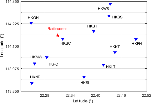
Figure 1Distribution of the Hong Kong SatRef sites (blue triangles) inside the tomography horizontal grid (black dotted lines) and the King's Park radiosonde station (red star). The region was discretized into an cell grid for the GPS water vapor tomography. The layer heights are 0, 400, 800, 1400, 2000, 2600, …, 8600 m from ground to water vapor layer top.
The reconstruction region covered an area ranging from latitude 22.22 to 22.52∘ N, longitude 113.85 to 114.35∘ E, and from ground to water vapor layer top (WVLT) in height. Thus, the entire area of Hong Kong was divided into 5×8 horizontal grids and 17 vertical layers. A total of voxels were divided in the 3-D space.
3.2 Regional weighted average temperature model
Bevis et al. (1994) first put forward the global Tm model using radiosonde products. Later, Wang et al. (2011) established the Tm model in Hong Kong using radiosonde products. Ye et al. (2016) also assessed the relationship between Tm and surface temperature based on radiosonde and COSMIC products. However, these three models only consider the parameter of surface temperature. We propose considering the effects of temperature and height to establish a Tm model using COSMIC products. The new model is given as follows (Yao et al., 2013):
where a, b, c, e and f are constants that can be determined using COSMIC products; Th indicates the temperature at height h; h denotes the height; and TmN is the new model value of Tm.
The weighted average temperature Tm is obtained using Eq. (9) with input wet pressure and temperature provided from wetPrfs. TmN can be derived using Eq. (15); its values are shown in Fig. 2. The wetPrfs described in Sect. 3.2 are used to derive the humidity conversion coefficient from Eq. (8).
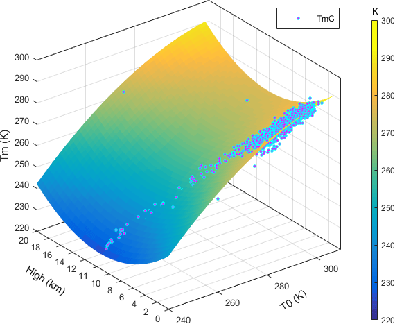
Figure 2Considering height and surface temperature to establish the Tm model using wetPrf products. T0 is the surface temperature, and TmC is the fitted atmospheric weighted average temperature obtained from COSMIC products for 2009 to 2015 in Hong Kong.
As shown in Fig. 2, the new model's Tm values agree well with the true values. To evaluate the new Tm model, its values are compared with those obtained from radiosonde and COSMIC products. Figure 3 shows the results for Hong Kong in August 2016.

Figure 3New Tm model values are compared with those derived from COSMIC and radiosonde products in Hong Kong in August 2016. TmC is the Tm derived from COSMIC products, TmN is the Tm derived from the new model, TmB is the Tm derived from the Bevis model, TmW is the Tm derived from the Wang model, and TmR is the Tm derived from radiosonde products.
The statistical results comparing the model-derived and COSMIC-derived Tm are given in Table 1. We provide a summary of the Tm deviation between radiosonde-derived and model-derived data in Table 2.
Table 1Summary of the Tm deviation between COSMIC-derived and model-derived (K) data.
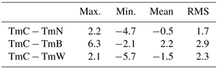
Table 2Summary of the Tm deviation between radiosonde-derived and model-derived (K) data.
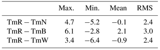
As shown in Tables 1 and 2, the new Tm model improves the accuracy of atmospheric weighted average temperature from the Bevis model and Wang model.
3.3 Tomography constraint condition
3.3.1 Estimating the smoothing factor
The smoothing factor δ in Eq. (10) is an uncertain parameter in the horizontal constraint. Usually, it is assigned a constant value of experience (Xia et al., 2013; Jiang et al., 2014). Because δ varies with regions and seasons and also changes with different levels of a tomography model, ERA-Interim data for Hong Kong from August 2009 to August 2015 were used to precisely estimate δ. ERA-Interim is a reanalysis of the global atmosphere covering the data period since 1989 and is continuing in real time (http://apps.ecmwf.int/datasets/data/, last access: 20 October 2017). The specific humidity data with 60 levels of vertical spatial resolution and a minimum grid of are publicly available. The main characteristics of the ERA-Interim system and many aspects of its performance are described in ECMWF newsletters 110, 115 and 119 (http://www.ecmwf.int/publications/newsletters, last access: 20 October 2017). In addition, comprehensive documentation of ERA-Interim, including observation usage, is currently being prepared and will be made available at http://www.ecmwf.int/research/era, last access: 20 October 2017.
Table 3Smoothing factor derived by ERA-Interim products at different heights.

In each level, the humidity information of one grid point equals the weighted average of its neighbors (Rius et al., 1997), as follows:
According to the humidity information provided by ERA-Interim, Eq. (16) can be solved using the optimal parameter search method. The search step is set to 1 and the search range is [0, 20]. The value of δ is exactly equal to the number of grid points in each level, and we defined the mean of δ as the smoothing factor of the level. Table 3 lists the δ values at different heights using ERA-Interim data for Hong Kong from August 2009 to August 2015.
Table 3 shows that the smoothing factors present a nonlinear change for increasing heights below 6 km, but do not change between 6 and 9 km. The horizontal constraint can be accurately determined based on the smoothing factor and the distance between known and unknown grids.
3.3.2 Vertical constraint
The purpose of GNSS tomography technique is to derive the 3-D distribution of water vapor. Thus, the accuracy of the vertical constraint will directly affect the quality of the tomography results. Because water vapor randomly varies in time and space, it is difficult to precisely probe the spatial distribution of water vapor. Traditionally, Eq. (14) was used as a vertical constraint and the parameter Hwe could be obtained using COSMIC or radiosonde historical data products (Ye et al., 2013, 2016). Due to Hwe changes over time are obvious, so they need to be obtained once for each tomography epoch. In this paper, PWV was derived using Eq. (4), and Hwe was then derived in real time based on Eq. (13). To evaluate the accuracy of Hwe, the radiosonde-obtained water vapor is used as a reference to assess the water vapor calculated using Eq. (11). The statistical results are given in Table 4 using the 45 004th radiosonde station (latitude: 22.32∘ N; longitude: 114.14∘ E) and HKSC station (latitude: 22.32∘ N; longitude: 114.14∘ E) datasets from August 2016 under 10 km.
Table 4Statistical results from Eq. (11)-derived and radiosonde-derived PWV (g m−3). RWV is the water vapor density obtained from the radiosonde product; TWV is the water vapor density derived from the Hwe obtained by the traditional method using Eq. (11); NWV is the water vapor density derived from the Hwe obtained by the new method using Eq. (11).
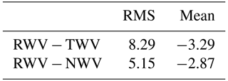
As shown in Table 4, the water vapor density derived from the Hwe obtained using the new technique and Eq. (11) is closer to the radiosonde-derived water vapor density. Therefore, it is more reasonable to use the Hwe obtained using the new technique and Eq. (14) as the vertical constraint.
To evaluate our optimized method, we obtained ZTDs from the Hong Kong SatRef network in August 2016, based on Bernese 5.2 (nondifference) software. The ZHDs were estimated using the Saastamoinen mode. The SWV was then obtained using the Niell mapping function (Niell, 1996) and the calibrated humidity conversion coefficient. The WVLT was determined as 9.5 km from COSMIC historical data and Ye et al.'s (2016) method. Following the tomography model proposed by Flores et al. (2000), we estimated the 3-D water vapor distribution using the GPS tomography technique with the horizontal constraint from Eq. (10) and the vertical constraint from Eq. (14). The tomography equation was solved by adopting Kalman filtering. The tomography results were outputted once every 30 min. As we have limited space, Fig. 4 only shows the 3-D distribution of water vapor density on 1 and 2 August 2016.
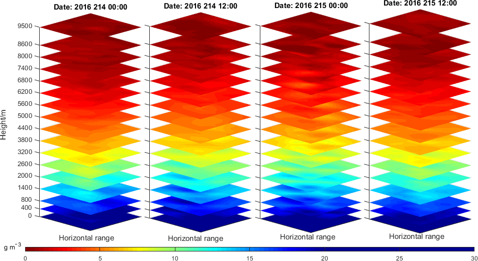
Figure 4 presents the 3-D tomographic water vapor distribution in Hong Kong for heights lower than 9.5 km. The results show that the water vapor changes significantly below 3.8 km, whereas it remains stable above 3.8 km. In addition, the water vapor is mainly concentrated below 2.6 km.
4.1 Compare the results between tomography-obtained and radiosonde-obtained data
Radiosonde products contain 3-D distribution of meteorological elements such as atmospheric temperature, atmospheric pressure, mixing ratio and relative humidity. The “wet” pressure can be obtained based on the pressure and mixing ratio and can be utilized to compute the water vapor density (Song, 2004). To verify the advantage of the optimized GPS tomography method, using radiosonde products as references, the tomography results were compared with those derived from the traditional tomography technique using the Saastamoinen dry model, a traditional humidity conversion coefficient (0.1538), a smoothing factor (Eq. 10), and Hwe obtained using the traditional technique and COSMIC historical products. Figure 5 compares the water vapor densities derived from radiosonde products and the traditional and optimized tomography techniques for 1 and 2 August 2016.
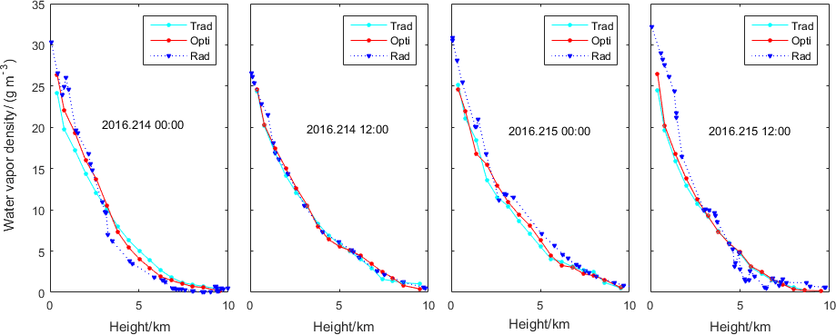
Figure 5Water vapor densities obtained from tomography-derived and radiosonde-derived data. Rad is the water vapor density derived using radiosonde products, Trad is the water vapor density derived using the traditional tomography method, and Opti is the water vapor density derived using the optimized method.
It can be observed in Fig. 5 that the changing trends of water vapor with height across the tomography-obtained and radiosonde-obtained data have a good agreement. However, when the “inversion layer” occurs, GPS tomography cannot accurately reflect this situation. In Table 5, we present the deviation statistics for GNSS tomography-obtained and radiosonde-obtained water vapor density at heights above and below 3.8 km, using 31-day datasets from Hong Kong over the whole of August 2016.
Table 5Statistics for tomography-derived and radiosonde-derived water vapor density above and below 3.8 km (g m−3). Rad is the radiosonde-derived water vapor density, Opti is the optimized tomography-derived water vapor density, and Trad is the traditional tomography-derived water vapor density.
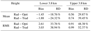
Table 5 provides the statistics values of the differences between GNSS tomography-obtained and radiosonde-obtained results. As seen from the statistical results, the root mean square (RMS) and mean values of troposphere tomography using the optimized technique is less than that based on the traditional method for altitudes below 3.8 km. In addition, compared with the radiosonde data, the test results show that the water vapor density quality obtained by the optimized technique is 13.8 % better below 3.8 km and 8.1 % better above 3.8 km than that obtained by the traditional technique.
4.2 Quality of GPS tomography technology
We also studied the differences in the entire humidity profile between the tomography-derived and radiosonde-derived results. We used the RMS and Pearson product-moment correlation coefficient (PCC) as the evaluation index correlated between the two profiles. PCC is a commonly used measure of the degree of correlation of two sequences of parameters, and the mathematical model is as follows (Lee and Nicewander, 1988):
Figure 6 presents the PCC and RMS of tomography results (traditional and optimized) for August 2016. Here we set up a set of criteria to evaluate the tomography profile PCC > 0.90 and RMS < 2.0 g m−3. When GPS tomography results meet these criteria, they are considered a success. According to the criteria, the success rate of the inversion is shown in Table 6.
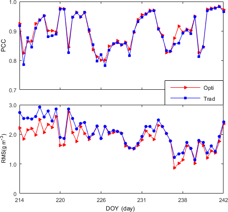
Figure 6Time series of PCC and RMS for August 2016. Opti is the optimized tomography-derived water vapor density, and Trad is the traditional tomography-derived water vapor density.
Table 6Statistical results of PCC and RMS for August 2016 (%).
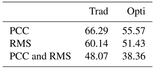
As shown in Table 6, the success rate of the optimized technique is nearly 10 % higher than that of the traditional technique, and the degree of improvement is evident. In fact, the principles of radiosonde and GPS tomography techniques are different. Radiosonde products reflect the state of the atmosphere at a certain time at the instrument's location, but GPS tomography techniques mirror the average water vapor state. Thus, it is difficult to determine an absolute standard to evaluate the success of GPS tomography results.
In this study, several key techniques in the GNSS tomography method were optimized to improve the accuracy of water vapor density. First, we re-established an atmospheric weighted average temperature model using COSMIC wetPrfs. According to the spatial distributions of water vapor provided by COSMIC products, we used the exponential model to fit the vertical variation of water vapor. The exponential function is usually utilized as the vertical constraint, and we proposed a new method to compute the scale height of water vapor. We determined the smoothing factor of the Gauss distance weighting function using ERA-Interim products. Finally, we used GPS datasets from Hong Kong in August 2016 to compute the PWV and the vertical distribution of water vapor density.
To evaluate the quality of the optimized technique, we compared the optimized and traditional technique results with radiosonde-obtained water vapor. The statistical results show that the water vapor density quality obtained by the optimized technique is 13.8 % better below 3.8 km and 8.1 % better above 3.8 km than that obtained by the traditional technique. We then calculated the success rate of tomographic inversion according to PCC and RMS. The statistics show that the success rate of the optimized technique was approximately 10 % higher than that of the traditional technique.
The Survey and Mapping Office of the Lands Department (2017), Hong Kong Special Administrative Region, provides GPS data and meteorological data. These datasets are from the Hong Kong Satellite Positioning Reference Station (SatRef) and can be made freely available for public access (https://www.geodetic.gov.hk/, last access: 14 September 2016). The 45 004 Kings Park radiosonde observations (University of Wyoming (UWYO), 2017) can be downloaded from the following website: http://weather.uwyo.edu/ upperair/sounding.html, last access: 20 October 2017. In addition, the Constellation Observing System for Meteorology, Ionosphere and Climate-1 program (CDAAC, 2017) offers the COSMIC radio occultation data, which can be freely obtained from ftp://cosmic-io.cosmic.ucar.edu/cdaac/index.html, last access: 20 October 2017.
PX conceived and designed the work that led to the submission; SY acquired data and played an important role in interpreting the results. PJ and LP drafted and revised the manuscript, and MG approved the final version.
The authors declare that they have no conflict of interest.
The financial support from the National 973 Program of China (no. 2012CB957701),
National Natural Science Foundation of China (no. 41074008), Key Laboratory
of Geospace Environment and Geodesy, Ministry of Education (no. 16-02-09),
and Henan Province 2018 Science and Technology Research Project (Science and
Technology/Industry) (no. 182102210315) are greatly
appreciated.
The topical editor,
Vassiliki Kotroni, thanks two anonymous referees for help in evaluating this
paper.
Bevis, M., Businger, S., Herring, T., Rocken, C., Anthes, R., and Ware, R.: GPS meteorology: Remote sensing of atmospheric water vapor using the global positioning system, J. Geophys. Res., 94, 15787–15801, 1992.
Bevis, M., Businger, S., Chiswell, S., Herring, T. A., Anthes, R. A., Rochen, C., and Ware, R. H.: GPS Meteorology: Mapping zenith wet delays onto precipitable water, J. Appl. Meteorol., 33, 379–386, 1994.
Beyerle, G., Schmidt, T., and Michalak, G.: GPS Radio Occultation with GRACE: Atmospheric profiling utilizing the zero difference technique, Geophys. Res. Lett., 32, L1386, https://doi.org/10.1029/2005GL023109, 2005.
CDAAC: Algorithms for inverting Radio Occultation signals in the neutral atmosphere, COSMIC Project Office, University Corporation for Atmospheric Research, available at: http://cosmic-io.cosmic.ucar.edu/cdaac/doc index.html (last access: 20 October 2017), 2005.
CDAAC: COSMIC Radio Occultation data, available at: http://cosmic-io.cosmic.ucar.edu/cdaac/index.html, last access: 20 October 2017.
Champollion, C., Masson, F., and Bouinm, N.: GPS water vapor tomography: Preliminary results from the ESCOMPTE field experiment, Atmos. Res., 74, 253–274, 2005.
Champollion, C., Flamant, C., Bock, O., Masson, F., Turner, D. D., and Weckwerth, T.: Mesoscale GPS tomography applied to the 12 June 2002 convective initiation event of IHOP_2002, Q. J. Roy. Meteorol. Soc., 135, 645–662, 2009.
Chen, G. and Herring, T. A.: Effects of atmospheric azimuthal asymmetry on the analysis of space Geodetic data, J. Geophys. Res., 102, 20489–20502, 1997.
Chen, B. and Liu., Z.: Voxel-optimized regional water vapor tomography and comparison with radiosonde and numerical weather model, J. Geodesy, 88, 691–703, 2014.
Davis, J. L., Herring, T. A., Shapiro, I. I., Rogers, A., and Elgered, G.: Geodesy by radio interferometry: Effects of atmospheric modeling errors on estimates of baseline length, Radio Sci., 20, 1593–1607, 1985.
Esteban, E., Vazquez, B., Borota, A., and Grejner, B.: GPS-PWV estimation and validation with radiosonde data and numerical weather prediction model in Antarctica, GPS Solut., 17, 29–39, 2013.
Falconer, R. H., Cobby, D., Smyth, P., Astle, G., Dent, J., and Golding, B.: Pluvial flooding: New approaches in flood warning, mapping and risk management, J. Flood Risk Manag., 2, 198–208, 2009.
Flores, A., Ruffini, G., and Rius, A.: 4D tropospheric tomography using GPS slant wet delays, Ann. Geophys., 18, 223–234, https://doi.org/10.1007/s00585-000-0223-7, 2000.
Hajj, G. A., Kursinski, E. R., Romans, L. J., Bertiger, W. I., and Leroy, S. S.: A technical description of atmospheric sounding by GPS occultation, J. Atmos. Sol.-Terr. Phy., 64, 451–469, 2002.
Jacob, D., Bärring, L., Christensen, O. B., Christensen, J. H., de Castro, Déqué, M. M., Giorgi, F., Hagemann, S., Hirschi, M., Jones, R., Kjellström, E., Lenderink, G., Rockel, B., Sánchez, E., Schär, C., Seneviratne, S. I., Somot, S., van Ulden, A., and van den Hurk, B.: An inter-comparison of regional climate models for Europe: model performance in present-day climate, Clim. Change, 81, 8479–8491, doi:10.1007/s10584-006-9213-4, 2007.
Jiang, P., Ye, S. R., Liu, Y. Y., Zhang, J. J., and Xia, P. F.: Near real-time water vapor tomography using ground-based GPS and meteorological data: long-term experiment in Hong Kong, Ann. Geophys., 32, 911–923, https://doi.org/10.5194/angeo-32-911-2014, 2014.
Jin, S. and Luo, O.: Variability and climatology of PWV from global 13-year GPS observations, IEEE T. Geosci. Remote, 47, 1918–1924, https://doi.org/10.1109/TGRS.2008.2010401, 2009.
Jin, S. G., Park, J., Cho, J., and Park, P.: Seasonal variability of GPS-derived Zenith Tropospheric Delay (1994-2006) and climate implications, J. Geophys. Res., 112. D09110, https://doi.org/10.1029/2006JD007772, 2007.
Jin, S. G., Li., Z. C., and Cho, J. H.: Integrated water vapor field and multi-scale variations over China from GPS measurements, J. Appl. Meteorol. Clim., 47, 3008–3015, https://doi.org/10.1175/2008JAMC1920.1, 2008.
Jin, S. G., Luo, O. F., and Gleason, S.: Characterization of diurnal cycles in ZTD from a decade of global GPS observations, J. Geodesy, 83, 537–545, https://doi.org/10.1007/s00190-008-0264-3, 2009.
Jin, S. G., Feng, G. P., and Gleason, S.: Remote sensing using GNSS signals: Current status and future directions, Adv. Space Res., 47, 1645–1653, https://doi.org/10.1016/j.asr.2011.01.036, 2011.
Kishore, P., Venkat, R., Namboothiric, S. P., Velicognaa, I., Bashab, G., Jiang, J. H., Igarashi, K., Rao, S. V. B., and Sivakumar, V.: Global (50∘ S–50∘ N) distribution of water vapour observed by Cosmic GPS Ro: Comparison with GPS Radiosonde, NCEP, Era-Interim, and Jra-25 reanalysis data sets, J. Atmos. Sol.-Terr. Phy., 73, 1849–1860, 2011.
Kouba, J. and Héroux, P.: Precise point positioning using IGS orbit and clock products, GPS Solut., 5, 12–28, 2001.
Kuo, B., Rocken, C., and Anthes, R.: GPS Radio Occultation Missions, The second Formosat3/COSMIC Data Users Workshop, 26–29 October 2007, Boulder, Colorado, 2007.
Kursinski, E. R., Hajj, G. A., and Schofield, J. T.: Observing Earth's atmosphere with Radio Occultation measurements using the Global Positioning System, J. Geophys. Res., 102, 23428–23465, 1997.
Lee, R. J. and Nicewander, W. A.: Thirteen ways to look at the correlation coefficient, Am. Stat., 42, 59–66, 1988.
Liou, Y. A., Pavelyev, A. G., Liu, S. F., Pavelyev, A. A., Yen, N., and Chen, J. F.: FORMOSAT-3/COSMIC GPS radio occultation mission: Preliminary results, IEEE T. Geosci. Remote, 45, 3813–3825, 2007.
MacMillan, D. S.: Atmospheric gradients from very long baseline interferometry observations, Geophys. Res. Lett., 22, 1041–1044, 1995.
Mateus, P., Nico, G., and Catalao, J.: Maps of PWV temporal changes by SAR interferometry: A study on the properties of atmosphere's temperature profiles, IEEE T. Geosci. Remote, 11, 2065–2069, 2014.
Niell, A. E.: Global mapping functions for atmosphere delay at radio wavelengths, J. Geophys. Res., 101, 3227–3246, 1996.
Nilsson, T. and Gradinarsky, L.: Water vapor tomography using GPS phase observation: Simulation results, IEEE T. Geosci. Remote, 44, 2927–2941, 2006.
Perler, D., Geiger, A., and Hurter, F.: 4D GPS water vapour tomography: New parameterized approaches, J. Geophys., 85, 539–550, https://doi.org/10.1007/s00190-011-0454-2, 2011.
Rius, A., Ruffini, G., and Cucurull, L.: Improving the vertical resolution of ionospheric tomography with GPS occultations, Geophys. Res. Lett., 24, 2291–2295, 1997.
Rocken, C., Anthes, R., Exner, M., Hunt, D., Sokolovskiy, S., and Ware, R.: Analysis and validation of GPS/MET data in the neutral atmosphere, J. Geophys. Res., 102, 29849–29866, 1997.
Shi, J. and Gao, Y.: Assimilation of GPS radio occultation observations with a near real-time GPS PPP-inferred water vapour system, P. ION GNSS, Savannah, Georgia, 2584–2590, 2009.
Song, S. L.: Sensing three dimensional water vapor structure with ground-based GPS network and the application in meteorology, PhD thesis of Shanghai Astronomical Observatory CAS, 80–84, 2004.
Troller, M., Geiger, A., Brockmann, E., and Kahle, H.-G.: Determination of the spatial and temporal variation of tropospheric water vapor using CGPS networks, Geophys. J. Int., 167, 509–520, 2006.
University of Wyoming (UWYO): 45004 Kings Park radiosonde observations, available at: http://weather.uwyo.edu/upperair/sounding.html, last access: 20 October 2017.
Wang, B.-R., Liu, X.-Y., and Wang, J.-K.: Assessment of COSMIC radio occultation retrieval product using global radiosonde data, Atmos. Meas. Tech., 6, 1073–1083, https://doi.org/10.5194/amt-6-1073-2013, 2013.
Wang, X., Song, L., Dai, Z., and Cao, Y.: Feature analysis of weighted mean temperature Tm in Hong Kong, J. Nanjing Univ. Info. Sci. Tech., 3, 47–52, 2011.
Xia, P., Cai, C., and Liu, Z.: GNSS troposphere tomography based on two-step reconstructions using GPS observations and COSMIC profiles, Ann. Geophys., 31, 1805–1815, https://doi.org/10.5194/angeo-31-1805-2013, 2013.
Yao, Y. B., Zhang, B., Yue, S. Q., Xu, C. Q., and Peng, W. F.: Global empirical model for mapping zenith wet delays onto precipitable water, J. Geodesy, 87, 439–448, https://doi.org/10.1007/s00190-013-0617-4, 2013.
Ye, S., Jiang, P., and Liu, Y.: A water vapor tomographic numerical quadrature approach with ground-based GPS network, Acta Geod. Cartogr. Sin., 42, 654–660, 2013.
Ye, S., Xia, P., and Cai, C.: Optimization of GPS water vapor tomography technique with radiosonde and COSMIC historical data, Ann. Geophys., 34, 789–799, https://doi.org/10.5194/angeo-34-789-2016, 2016.