Transfer entropy and cumulant-based cost as measures of nonlinear causal relationships in space plasmas: applications to D_st

It is well known that the magnetospheric response to the solar wind is nonlinear. Information theoretical tools such as mutual information, transfer entropy, and cumulant-based analysis are able to characterize the nonlinearities in the system. Using cumulant-based cost, we show that nonlinear significance of D_st peaks at 3–12 h lags that can be attributed to VB_s, which also exhibits similar behavior. However, the nonlinear significance that peaks at lags 25, 50, and 90 h can be attributed to internal dynamics, which may be related to the relaxation of the ring current. These peaks are absent in the linear and nonlinear self-significance of VB_s. Our analysis with mutual information and transfer entropy shows that both methods can establish that there are strong correlations and transfer of information from V_sw to D_st at a timescale that is consistent with that obtained from the cumulant-based analysis. However, mutual information also shows that there is a strong correlation in the backward direction, from D_st to V_sw, which is counterintuitive. In contrast, transfer entropy shows that there is no or little transfer of information from D_st to V_sw, as expected because it is the solar wind that drives the magnetosphere, not the other way around. Our case study demonstrates that these information theoretical tools are quite useful for space physics studies because these tools can uncover nonlinear dynamics that cannot be seen with the traditional analyses and models that assume linear relationships.

1 Introduction

One of the most practically important concepts in dynamical systems is the notion of causality. It is particularly useful to organize observational datasets according to causal relationships in order to identify variables that drive the dynamics. Understanding causal dependencies can also help to simplify descriptions of highly complex physical processes because it constrains the coupling functions between the dynamical variables. Analysis of those coupling functions can lead to simplification of the underlying physical processes that are most important for driving the system. It is particularly useful from a practical standpoint to understand causal dependencies in systems involving natural hazards because monitoring of causal variables is closely linked with warning.

A common method to establish causal dependencies in a data stream of two variables, e.g., [a(t)] and [b(t)], is to apply linear correlation studies such as Strangeway et al. (2005), which showed the relationship between the downward Poynting flux and ion outflows. Causal relationships are typically identified by considering a time-shifted correlation function

$$\begin{array}{}\text{(1)}& {\mathit{\lambda }}_{ab}\left(\mathit{\tau }\right)\mathit{\triangleq }{\displaystyle \frac{\langle a\left(t\right)b(t+\mathit{\tau })\rangle -\langle a\rangle \langle b\rangle }{\sqrt{\langle a^{\mathrm{2}}\rangle -\langle a{\rangle }^{\mathrm{2}}}\sqrt{\langle b^{\mathrm{2}}\rangle -\langle b{\rangle }^{\mathrm{2}}}}},\end{array}$$

where 〈…〉 is an ensemble average obtained by drawing samples at a set of measurement times, $\mathit{\{}{t}_{\mathrm{0}},t_{\mathrm{1}},\mathrm{\dots },t_N\mathit{\}}$. For example, Borovsky et al. (1998) used such a method to identify relationships between solar wind variables and plasma sheet variables. The causal dependency that the plasma sheet responds to changes in the solar wind can be identified from the time-shift of the peak of the cross-correlation indicating a response time. From this type of analysis it can be found that the plasma sheet generally responds from the tail to the inner magnetosphere, consistent with the notion of earthward convection. Such analysis has been particularly useful to help understand plasma sheet transport.

However, the procedure of detecting causal relationships based on linear cross-correlation suffers from a number of limitations. First it should be noted that the statistical accuracy of the correlation function is limited by the resolution and length of the data stream. Second, the linear time series analysis ignores nonlinear correlations, which may be important for energy transfer in the magnetospheric system. For example, substorms are believed to involve storage and release of energy in the magnetotail, which is a highly nonlinear response. Similarly, magnetosphere–ionosphere coupling may also be highly nonlinear, involving the nonlinear development of accelerating potentials along auroral field lines and nonlinear current–voltage relationships. Third, the cross-correlation may not be a particularly clear measure when there are multiple peaks or if there is little or no asymmetry in the forward (i.e., λ_ab(τ)) and backward directions (i.e., ${\mathit{\lambda }}_{ba}\left(\mathit{\tau }\right)={\mathit{\lambda }}_{ab}(-\mathit{\tau })$). Finally, the cross-correlation does not provide any way to clearly distinguish between two variables that are passively correlated because of a common driver rather than causally related.

In the remainder of this paper, we will discuss other methods to identify causal relationships based on entropy-based discriminating statistics such as mutual information and transfer entropy. We will also discuss the cumulant-based method. We will illustrate the shortcomings and strengths of the various methods for studying causality with examples from nonlinear dynamics and space physics.

2 Linear vs. nonlinear dependency

It is well known that the magnetosphere responds to variation in the solar wind parameters (Baker et al., 1983; Clauer et al., 1981; Crooker and Gringauz, 1993; Johnson and Wing, 2015; Papitashvili et al., 2000; Wing and Johnson, 2015; Wing et al., 2016), and it has been established that the magnetosphere has a significant linear response to the solar wind. However, it is also expected that the magnetosphere has a nonlinear response (Balikhin et al., 2011; Klimas et al., 1998; Tsurutani et al., 1990; Valdivia et al., 2013; Vassiliadis et al., 1990). The nonlinear response may be driven by internal dynamics rather than being driven externally (Johnson and Wing, 2005; Wing et al., 2005). For example, the internal dynamics associated with loading and unloading of magnetic energy associated with storms and substorms is nonlinear (Johnson and Wing, 2014). Indeed, the data analysis of Bargatze et al. (1985) indicated that the dynamical response of the magnetosphere to solar wind input could not be entirely understood using linear prediction filters.

Suppose that we consider a set of variables a and b, which could be vectors of variables measured in time and we would like to measure their dependency. Instead of considering the covariance matrix or correlation function, we consider a more general measure of dependency between an input and output is obtained by considering whether

$$\begin{array}{}\text{(2)}& P(\mathit{a},\mathit{b})\stackrel{\mathrm{?}}{=}P\left(\mathit{a}\right)P\left(\mathit{b}\right),\end{array}$$

where P(a,b) is the joint probability of input a and output b, while P(a) and P(b) are the probability of a and b respectively. If the relationship holds, then the variables a and b are independent. For all other cases, there is some measure of dependency. In the case where the system output is completely known given the input, $P(\mathit{a},\mathit{b})=P\left(\mathit{a}\right)$. The advantage of considering Eq. (2) is that it is possible to detect the presence of higher order nonlinear dependencies between the input and output even in the absence of linear dependencies (Gershenfeld, 1998).

2.1 Mutual information and cumulant-based cost

Mutual information and cumulant-based cost are two useful measures that quantify Eq. (2). Mutual information has the advantage that in the limit of Gaussian joint probability distributions, it may be simply related to the correlation coefficient C_ab(τ) defined in Eq. (1) (Li, 1990). Cumulants have the advantage of good statistics for limited datasets and noisy systems (Deco and Schürmann, 2000). Moreover, for high-dimensional systems it is more efficient to compute moments of the data rather than try to construct the probability density function.

Correlation studies also only detect linear correlations, so if the feedback involves nonlinear processes (highly likely in this case) then their usefulness may be seriously limited. Alternatively, entropy-based measures such as mutual information (Materassi et al., 2011; Prichard and Theiler, 1995) and cumulants (Johnson and Wing, 2005) are useful for detecting linear as well as nonlinear correlations. The mutual information is constructed from the probability distribution function of the variables and may be computed using a quantization procedure where data are binned such that the samples [a(t)] are assigned discrete values $\widehat{a}\in \mathit{\{}{a}_{\mathrm{1}},a_{\mathrm{2}},\mathrm{\dots },a_n\mathit{\}}$ of an alphabet ℵ₁ and [b(t)] is assigned discrete values $\widehat{b}\in \mathit{\{}{b}_{\mathrm{1}},b_{\mathrm{2}},\mathrm{\dots },b_m\mathit{\}}$ of an alphabet ℵ₂. The ad hoc time-shifted mutual entropy

$$\begin{array}{ll}{\displaystyle }& {\displaystyle }{\mathcal{M}}_{ab}\left(\mathit{\tau }\right)\mathit{\triangleq }\\ \text{(3)}& {\displaystyle }& {\displaystyle }\sum _{\widehat{a}\in {\mathrm{\aleph }}_{\mathrm{1}},\widehat{b}\in {\mathrm{\aleph }}_{\mathrm{2}}}p\left(\widehat{a}\right(t+\mathit{\tau }),\widehat{b}(t\left)\right)\log \left({\displaystyle \frac{p\left(\widehat{a}\right(t+\mathit{\tau }),\widehat{b}(t\left)\right)}{p\left(\widehat{a}\right)p\left(\widehat{b}\right)}}\right)\end{array}$$

has been used as an indicator of causality, but suffers from the same problems as the time-shifted cross-correlation when it has multiple peaks and long-range correlations.

Similarly, examination of time-shifted cumulants could be used as an indicator of causality in a nonlinear system. In this case, we can define a discriminating statistic

$$\begin{array}{}\text{(4)}& D^C=\sum _{q=\mathrm{1}}^{\mathrm{\infty }}\sum _{i_{\mathrm{1}},\mathrm{\dots },i_q\in {\mathrm{\Pi }}_q}{K}_{\mathrm{1}{i}_{\mathrm{2}}\mathrm{\dots }{i}_q}^{\mathrm{2}},\end{array}$$

where

$$\begin{array}{}\text{(5)}& {\displaystyle }\begin{array}{lcl}{K}_i& =& C_i=\langle z_i\rangle \\ K_{ij}& =& C_{ij}-C_i{C}_j=\langle z_i{z}_j\rangle -\langle z_i\rangle \langle z_j\rangle \\ K_{ijk}& =& C_{ijk}-C_{ij}{C}_k-C_{jk}{C}_i-C_{ik}{C}_j+\mathrm{2}{C}_i{C}_j{C}_k\\ K_{ijkl}& =& C_{ijkl}-C_{ijk}{C}_l-C_{ijl}{C}_k-C_{ilk}{C}_j-C_{ljk}{C}_i\\ & & -C_{ij}{C}_{kl}-C_{il}{C}_{kj}-C_{ik}{C}_{jl}+\mathrm{2}(C_{ij}{C}_k{C}_l\\ & & +C_{ik}{C}_j{C}_l+C_{il}{C}_j{C}_k+C_{jk}{C}_i{C}_l+C_{jl}{C}_i{C}_k\\ & & +C_{kl}{C}_i{C}_j)-\mathrm{6}{C}_i{C}_j{C}_k{C}_l\end{array}\end{array}$$

are the cumulants

$$\begin{array}{}\text{(6)}& C_{i\mathrm{\dots }j}=\int \mathrm{d}\mathit{z}P\left(\mathit{z}\right)z_i\mathrm{\dots }{z}_j\equiv \langle z_i\mathrm{\dots }{z}_j\rangle \end{array}$$

of the joint probability distribution for variables $z_{\mathrm{1}},\mathrm{\dots },z_j$.

With only two variables, a and b, defined above, we can consider the cost function

$$\begin{array}{}\text{(7)}& D_{a,b}^C\left(\mathit{\tau }\right)=D^C\left(a\right(t),b(t+\mathit{\tau }\left)\right).\end{array}$$

The presence of nonlinear dependence has been identified by comparing the cumulant cost for a time series with the cumulant-based cost of surrogate time series, which are constructed to have the same linear correlations as in Johnson and Wing (2005). Significance measures the difference in the discriminating statistic from the mean of the discriminating statistic of the surrogates in terms of the spread of the surrogates, σ.

In Sect. 3, we will show an application of cumulant-based analysis to the disturbance storm time index (D_st). In principle, the cross-correlation, mutual information, and cumulant-based cost should be independent of the selection of measurement points if the system is stationary; therefore, time stationarity can be examined by comparing these discriminating statistics for groups of measurements drawn from different windows of time as in Johnson and Wing (2005) and Wing et al. (2016).

2.2 Transfer entropy

Another method for determining causality is the one-sided transfer entropy (De Michelis et al., 2011; Materassi et al., 2014; Schreiber, 2000; Wing et al., 2016, 2018), which is based upon the conditional mutual information

$$\begin{array}{ll}{\displaystyle }& {\displaystyle }{\mathcal{M}}_C(x,y|z)\mathit{\triangleq }\\ \text{(8)}& {\displaystyle }& {\displaystyle }\sum _{x\in {\mathrm{\aleph }}_{\mathrm{1}}}\sum _{y\in {\mathrm{\aleph }}_{\mathrm{2}}}\sum _{z\in {\mathrm{\aleph }}_{\mathrm{3}}}p(x,y,z)\log \left({\displaystyle \frac{p(x,y,z)p\left(z\right)}{p(x,z)p(y,z)}}\right).\end{array}$$

The conditional mutual information measures the dependence of two variables, x and y, given a conditioner variable, z. If either x or y are dependent on z, the mutual information between x and y is reduced, and this reduction of information provides a method to eliminate coincidental dependence, or conversely to identify causal dependence.

Transfer entropy considers the conditional mutual information between two variables using the past history of one of the variables as the conditioner.

$$\begin{array}{ll}{\displaystyle }& {\displaystyle }{\mathcal{T}}_{a\to b}\left(\mathit{\tau }\right)=\sum _{\widehat{a}\in {\mathrm{\aleph }}_{\mathrm{1}}}\sum _{{\widehat{a}}^{\left(k\right)}\in {\mathrm{\aleph }}_{\mathrm{1}}^{\left(k\right)}}\sum _{\widehat{b}\in {\mathrm{\aleph }}_{\mathrm{2}}}p\left(\widehat{a}\right(t+\mathit{\tau }),{\widehat{a}}^{\left(k\right)}(t),\widehat{b}(t\left)\right)\\ \text{(9)}& {\displaystyle }& {\displaystyle }\log \left({\displaystyle \frac{p\left(\widehat{a}\right(t+\mathit{\tau }\left)\mathrm{|}{\widehat{a}}^{\left(k\right)}\right(t),\widehat{b}(t\left)\right)}{p\left(\widehat{a}\right(t+\mathit{\tau }\left)\mathrm{|}{\widehat{a}}^{\left(k\right)}\right(t\left)\right)}}\right),\end{array}$$

where ${\widehat{a}}^{\left(k\right)}\left(t\right)=\left[\widehat{a}\right(t),\widehat{a}(t-\mathrm{\Delta }),\mathrm{\dots },\widehat{a}(t-(k-\mathrm{1})\mathrm{\Delta }\left)\right]$. The standard definition of transfer entropy takes k=1 (no lag), but keeping a higher embedding dimension could in principle provide a more precise measure (for example, if a has periodicity, a dimension of 2 may provide better prediction of future values of a from its past time series and therefore lower the transfer entropy). Transfer entropy as a discriminating statistic has the following advantages. First, in the absence of information flow from a to b (i.e., a(t+τ) has no additional dependence from b(t) beyond what is known from the past history of a^(k)(t)) so that $p\left(\widehat{a}\right(t+\mathit{\tau }\left)\mathrm{|}{\widehat{a}}^{\left(k\right)}\right(t),\widehat{b}(t\left)\right)=p\left(\widehat{a}\right(t+\mathit{\tau }\left)\mathrm{|}{\widehat{a}}^{\left(k\right)}\right(t\left)\right)$ and the transfer entropy vanishes. The transfer entropy is also highly directional so that ${\mathcal{T}}_{a\to b}\ne {\mathcal{T}}_{b\to a}$. The advantage can be clearly seen for dynamical systems in which variables are forward differenced and the transfer entropy is clearly one-sided while mutual information and correlation functions can even be symmetric (Schreiber, 2000). This measure also accounts for static internal correlations, which can be used to determine whether two variables are driven by a common driver or whether the variable b is causally driving the variable a.

Both mutual information and transfer entropy require binning of data. As mentioned in Wing et al. (2016), the number of bins (n_b) needs to be chosen properly and there are some guidelines that can be followed. In general, we would like to maximize the amount of information. Having too few bins would lump too many points into the same bin, leading to loss of information. Conversely, having too many bins would leave many bins with 0 or a few number of points, which also would lead to loss of information. Sturges (1926) proposed that for a normal distribution, optimal $n_{\mathrm{b}}={\log }_{\mathrm{2}}\left(n\right)+\mathrm{1}$ and bin width w = range∕n_b, where n is the number of points in the dataset and range is the maximum value minus the minimum value of the points. In practice, there is usually a range of n_b that would work.

3 Application to space weather: D_st analysis

D_st (disturbance storm time index) is an hourly index that gives a measure of the strength of the symmetric ring current that, in turn, provides a measure of the dynamics of geomagnetic storms (Dessler and Parker, 1959). Because of its global nature, D_st is often used as one of the several indices that represent the state of the magnetosphere. For example, Balasis et al. (2011) used the cumulative square amplitude of the D_st time series as a proxy for energy dissipation rate in the magnetosphere and found that it fits a power law well with log-periodic oscillations, which was interpreted as evidence for discrete-scale invariance in the D_st dynamics.

When plasma sheet ions are injected into the Earth's inner magnetosphere, they drift westward around the Earth, forming the ring current. Studies have shown that the substorm occurrence rate increases with solar wind velocity (high speed streams) (Kissinger et al., 2011; Newell et al., 2016). An increase in the solar wind electric field, VB_z, can increase the dawn–dusk electric field in the magnetotail, which in turn determines the number of plasma sheet particles that move to the inner magnetosphere (Friedel et al., 2001). Studies have shown that the electric field, VB_s (V_sw × southward IMF B_z) or VB_z, has a strong effect on the ring current dynamics (Burton et al., 1975; McPherron and O'Brien, 2001; O'Brien and McPherron, 2000; Weygand and McPherron, 2006).

For the present study, we examine the relationships between solar wind velocity (V_sw) and VB_s with D_st. We use D_st records in the period 1974–2001 obtained from Kyoto University World Data Center for Geomagnetism (http://swdcwww.kugi.kyoto-u.ac.jp/index.html, last access: 18 January 2018). The corresponding solar wind data are obtained from IMP-8, ACE, WIND, ISEE1, and ISEE3 observations. The ACE SWEPAM and MAG data and the WIND MAG data are obtained from CDAWeb (http://cdaweb.gsfc.nasa.gov/, last access: 18 January 2018). The WIND 3DP data are obtained from the 3DP team directly. The ISEE1 and ISEE3 data are obtained from UCLA (these datasets are also available at NASA NSSDC; http://nssdc.gsfc.nasa.gov/space/, last access: 18 January 2018). The IMP8 data come directly from the IMP teams. The solar wind is propagated with the minimum variance technique (Weimer et al., 2003) to GSM (X, Y, Z) = (17, 0, 0) R_E to produce 1 min files, from which hourly averaged solar wind parameters are constructed.

3.1 Cumulant-based analysis

Section 2.1 presents the method of cumulant-based cost. Here, we show an application of cumulant-based cost to detect nonlinear dynamics in D_st. We consider the forward coupling between a solar wind variable such as VB_s and D_st, which characterizes the ring current response to the solar wind driver. We therefore consider the nonlinear cross-correlations of the vector

$$\begin{array}{}\text{(10)}& \mathit{c}(t,\mathit{\tau })=\mathit{\left\{}{\mathit{\text{VB}}}_{\mathrm{s}}\right(t),D_{\mathrm{st}}(t+\mathit{\tau }\left)\mathit{\right\}}=\mathit{\{}{z}_{\mathrm{1}},z_{\mathrm{2}}\mathit{\}}.\end{array}$$

The generalization of cost is based on realizations of {z₁,z₂}. In this case, each variable is Gaussianized with unit variance to eliminate static nonlinearities (i.e., higher order self-correlations in VB_s and D_st are eliminated so that the cost measures only cross-dependence between VB_s and D_st). This procedure is explained in the next paragraph.

The distributions of D_st and VB_s are generally non-Gaussian. As such, the raw distributions (e.g., distribution of values of D_st) may have nonzero higher order cumulants (e.g., they can have a skew and kurtosis). This property makes it more difficult to interpret whether the higher order cumulants in the time evolution arise from the overall shape of the distribution of data points or from the time-ordering of the data. To eliminate the inherent nonzero cumulants in the overall distribution of data, we construct a rank-ordered map from the original dataset to a proxy dataset of the same length drawn from a Gaussian distribution (Deco and Schürmann, 2000; Kennel and Isabelle, 1992; Schreiber and Schmitz, 1996). The distribution of the proxy dataset ensures that all cumulants of the distribution beyond second order should in principle vanish. However, the time-ordering of the data can still lead to nonzero cumulants because the joint probability distribution of D_st(t+τ) and D_st(t) may be non-Gaussian even if the distribution of D_st is Gaussian. Moreover, it is simple to construct surrogate data from the Gaussianized data that share the same autocorrelation by using the same power spectrum but randomly shifting the phases of the Fourier coefficients. The surrogate data therefore have the same autocorrelation as the original data. Any deviation from the linear statistic is apparent from comparison with the surrogate data, and we interpret these deviations as evidence of nonlinear dependence because we have falsified the hypothesis that the data can be adequately described by linear statistics. This method has been successfully employed in Johnson and Wing (2005), in which the K_p record was analyzed with mutual information and cumulants.

In Fig. 1 we plot the significance obtained from the year 1999 as a function of time delay, τ. Significance extracted from $\mathit{\left\{}{\mathit{\text{VB}}}_{\mathrm{s}}\right(t),D_{\mathrm{st}}(t+\mathit{\tau }\left)\mathit{\right\}}$ and $\mathit{\left\{}{\mathit{\text{VB}}}_{\mathrm{s}}\right(t),{\mathit{\text{VB}}}_{\mathrm{s}}(t+\mathit{\tau }\left)\mathit{\right\}}$ for 1999 is plotted in panels (a) and (b), respectively. It should be noted that there is a strong linear response at around 3 h time delay. As shown in Fig. 1a, there is a clear nonlinear response with peaking around 3–10, 25, 50, and 90 h, lasting for approximately 1 week. In contrast, in Fig. 1b, the nonlinearity only has one broad peak around 3–12 h in the self-significance for VB_s, suggesting that the nonlinear and linear peaks at τ=3–12 h in Fig. 1a may be associated with VB_s. We will revisit the solar wind causal relationship with D_st using transfer entropy in Sect. 3.2.

The absence of the nonlinear peaks at τ = 25, 50, and 90 h in the self-significance for VB_s (Fig. 1b) suggests that these nonlinearities in $\mathit{\left\{}{\mathit{\text{VB}}}_{\mathrm{s}}\right(t),D_{\mathrm{st}}(t+\mathit{\tau }\left)\mathit{\right\}}$ are related to internal magnetospheric dynamics. As the D_st index is thought to reflect storm activity, it is reasonable that nonlinear significance would decay on the order of 1 week as storms commonly last around that time. The strong nonlinear responses at τ = 25, 50, and 90 h are likely related to multiple modes of relaxation of the ring current following the commencement of storms. It should also be noted that other nonlinearities detected by even higher order cumulants may also be present; however, the calculation demonstrates the nonlinear nature of the underlying dynamics.

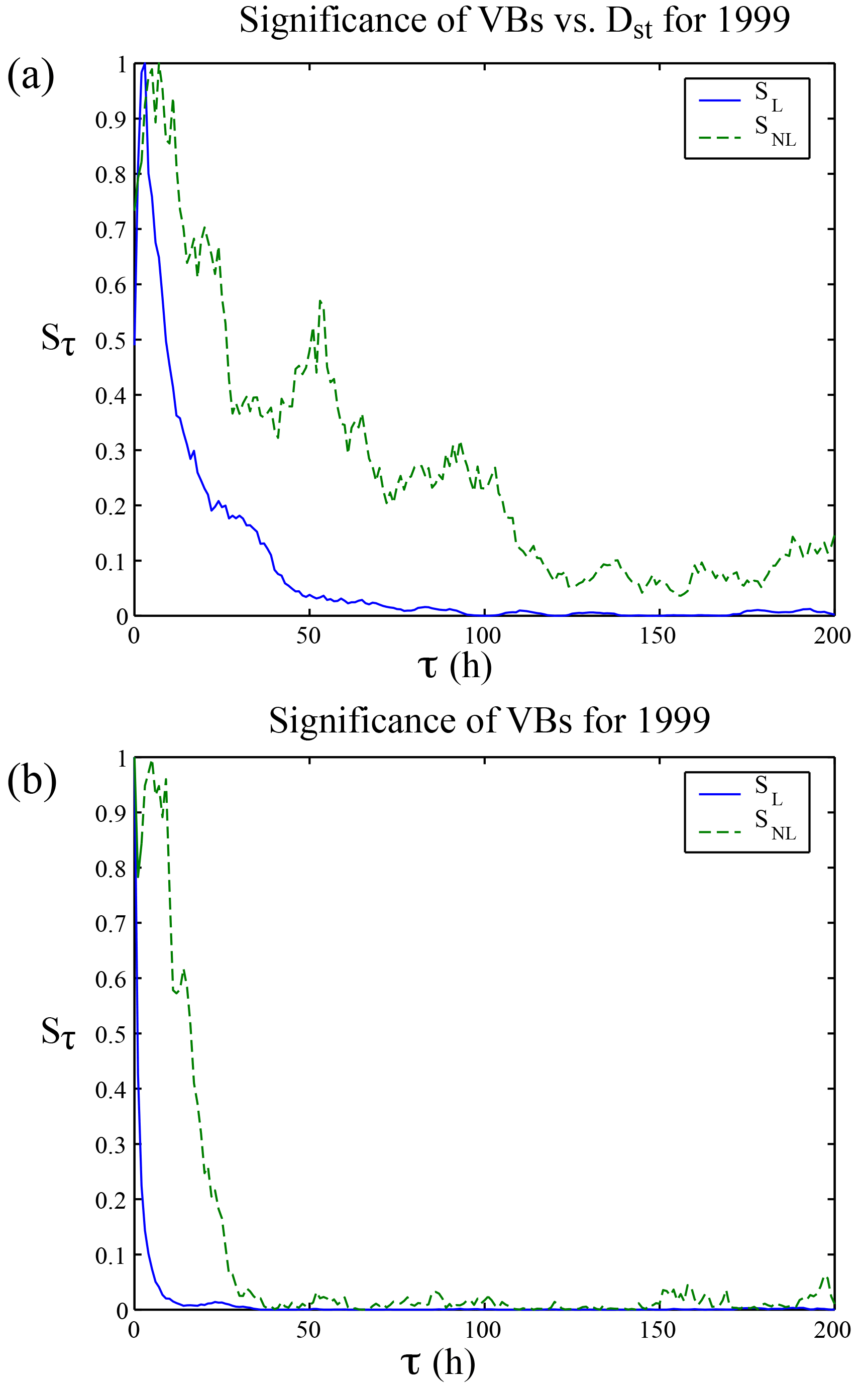
Figure 1 Significance extracted from (a) $\mathit{\left\{}{\mathit{\text{VB}}}_{\mathrm{s}}\right(t),D_{\mathrm{st}}(t-\mathit{\tau }\left)\mathit{\right\}}$ and (b) $\mathit{\left\{}{\mathit{\text{VB}}}_{\mathrm{s}}\right(t),{\mathit{\text{VB}}}_{\mathrm{s}}(t-\mathit{\tau }\left)\mathit{\right\}}$ for 1999. It should be noted that there is a strong linear response at around 3 h time delay. There is a clear nonlinear response with a strong peak around 50 h lasting for approximately 1 week. The long-term nonlinear response is absent in the solar wind data, indicating that the long-term nonlinear correlations between VB_s and D_st are the result of internal magnetospheric dynamics.

A common scenario for storm–ring current interaction is the following. A storm compresses the magnetosphere, intensifies the magnetic field in the magnetosphere, and injects energetic particles into the ring current region. The ring current intensifies during the main phase of the storm, which can last ∼ 6 h (Weygand and McPherron, 2006). Once the injection stops, the ring current begins to decay and the storm enters the recovery phase. Conservation of the magnetic moment implies that anisotropies develop in the ring current and plasma sheet. Anisotropy drives the ring current plasma unstable to ion cyclotron waves. The ion cyclotron waves scatter energetic ions into the loss cone so that they are lost from the ring current. Nonlinear interaction between waves and particles keeps the plasma near marginal stability with a steady loss of energetic particles due to wave–particle scattering. Other loss mechanisms include charge exchange, Coulomb scattering, and convection of ions to the front of the magnetopause. The ring current decay can have two stages (Kozyra et al., 2002). In the first stage, the ring current decays rapidly and the loss mechanisms can be attributed to convective outflow, pitch-angle scattering in the ring current, and O⁺ charge exchange (Hamilton et al., 1988; Weygand and McPherron, 2006). The second stage may typically begin about 1 day from the commencement of the storm (see, for example, Fig. 7 of Kozyra et al., 2002). In the second stage, the decay rate is slower and is attributed mainly to H⁺ charge exchange (Hamilton et al., 1988) and can take several days to deplete the ring current to the baseline level (Smith et al., 1976). We can speculate that the multiple nonlinear response lag times that are detected with the cumulant-based approach are likely the relaxation of the ring current due to the complex interplay of multiple loss processes.

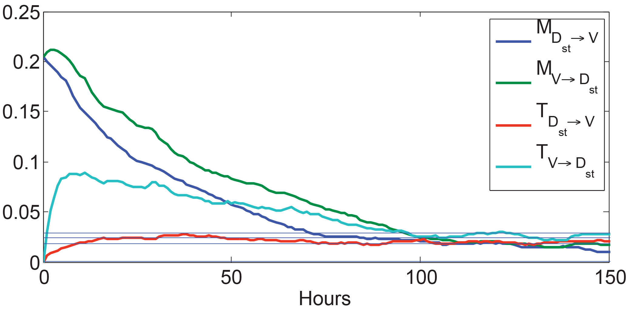
Figure 2 Comparison of mutual information and transfer entropy measures to determine causal driving of the magnetosphere as characterized by D_st. Note that causal driving appears to peak somewhat later (11 h) than indicated by mutual information (2 h), indicating that internal dynamics likely are very important initially. The backward transfer entropy is below the noise level for all values, indicating that D_st in no way influences the upstream solar wind velocity. Such a conclusion could not be inferred from the mutual information measure.

3.2 Transfer entropy

As mentioned in Sect. 2.2, transfer entropy gives a measure of how much information is transferred from one variable to another. We have applied transfer entropy and mutual information to the relationship between the V_sw and D_st for the period 1974–2001. The result is shown in Fig. 2. Note that the mutual information measure suggests strong correlations between prior values of D_st and V_sw. This finding suggests that D_st could be a driver of V_sw, which is counterintuitive. On the other hand, the transfer entropy clearly shows that this information transfer in the backward direction (D_st→V_sw) does not rise above the noise level (the horizontal blue lines indicate mean and standard deviation of 100 surrogate datasets for which the data were randomly reordered.) This result is expected because it is the solar wind that drives the magnetosphere, not the other way around. The transfer of information from V_sw to D_st peaks at τ=8–11 h. The cumulant-based analysis in Sect. 3.1 shows that the response of D_st to VB_s has a similar timescale. This timescale is consistent with the 4 to 15 h transport time for the solar wind to reach the midnight and noon regions of the geosynchronous orbit, respectively, from the dayside magnetopause (Borovsky et al., 1998). The analysis presented here illustrates the power of the transfer entropy for accessing causality.

4 Summary

We recently used mutual information, transfer entropy, and conditional mutual information to discover the solar wind drivers of the outer radiation belt electrons (Wing et al., 2016). Because V_sw anticorrelates with solar wind density (n_sw), it is hard to isolate the effects of V_sw on radiation belt electrons, given n_sw and vice versa. However, using conditional mutual information, we were able to determine the information transfer from n_sw or any other solar wind parameters to radiation belt electrons, given V_sw (or any other solar wind parameters). We also showed that the triangle distribution in the radiation belt electron vs. solar wind velocity plot (Reeves et al., 2011) can be understood better when we consider that V_sw and n_sw transfer information to radiation belt electrons with lags of 2 and 0 days (< 24 h), respectively. Also recently, we used transfer entropy to better understand the causal parameters in the solar cycle dynamo and their response lag times (Wing et al., 2018).

As a follow-up to Wing et al. (2016, 2018), the present study demonstrates further how information theoretical tools can be useful for space physics and space weather studies. Cumulant-based analysis can be used to distinguish internal vs. external driving of the system. Both mutual information and transfer entropy give a measure of shared information between two variables (or vectors). However, unlike mutual information, transfer entropy is highly directional. To illustrate, we apply mutual information, transfer entropy, and cumulant-based analysis to investigate the dynamics of the D_st index.

Our analysis with mutual information and transfer entropy indicates that there are strong linear and nonlinear correlations and transfer of information, respectively, in the forward direction between V_sw and D_st (V_sw → D_st). However, mutual information indicates that there is also a strong correlation in the backward direction (D_st → V_sw), which is puzzling and counterintuitive. In contrast, the transfer entropy indicates that there is no information transfer in the backward direction (D_st→V_sw), as expected because it is the solar wind that drives the magnetosphere, not the other way around. The transfer of information from V_sw to D_st peaks at τ=8–11 h.

Using the cumulant-based significance, we have established that the underlying dynamics of D_st is in general nonlinear, exhibiting a quasiperiodicity which is detectable only if nonlinear correlations are taken into account. The strong nonlinear responses of D_st to VB_s at τ=25, 50, and 90 h are likely related to multiple modes of relaxation of the ring current from multiple loss mechanisms following the commencement of storms. It is, of course, possible that these nonlinearities are caused by solar wind drivers other than VB_s. However, the timing of these nonlinearities would put them well in the recovery phase of a storm, and previous studies suggested that the ring current decays in the recovery phase are strongly influenced by VB_s (Burton et al., 1975; McPherron and O'Brien, 2001; O'Brien and McPherron, 2000). The nonlinearities at τ=3–12 h are not caused by internal dynamics but rather by the solar wind driver, which is similar to the timescale for the solar wind transport time from the dayside magnetopause to the inner magnetosphere. This timescale is consistent with the timescale for the information transfer from the solar wind to D_st obtained from transfer entropy analysis.

Although linear models are useful, our results indicate that these models have to be used with caution because the solar wind–magnetosphere system is inherently nonlinear. Hence, nonlinearities generally need to be taken into account in order to describe the system accurately. Local linear models (which include slow evolution of parameters) may be able to handle some nonlinearities, but it is expected that these local linear models would have difficulties if the dynamics suddenly and rapidly change.