the Creative Commons Attribution 4.0 License.
the Creative Commons Attribution 4.0 License.
 | 14 Jun 2018
A statistical study of the spatial distribution and source-region size of chorus waves using Van Allen Probes data
Shangchun Teng
Xin Tao
Wen Li
Xinliang Gao
Quanming Lu
Shui Wang
The spatial distribution and source-region size of chorus waves are important parameters for understanding their generation. In this work, we analyze over 3 years of continuous wave burst-mode data from the Van Allen Probes mission and build a data set of rising-tone and falling-tone chorus waves. For the L shell range covered by Van Allen Probes data (), statistical results demonstrate that the sector where rising tones are most likely to be observed is the dayside during geomagnetically quiet and moderate times and the dawn side during active times. Moreover, rising-tone chorus waves have a higher occurrence rate near the equatorial plane, while the falling-tone chorus waves have a higher possibility to be observed at lower L shell and higher magnetic latitudes. By analyzing the direction of the Poynting wave vector, we statistically investigate the chorus source-region size along a field line, and compare the results with previous theoretical estimates. Our analysis confirms previous conclusions that both rising-tone and falling-tone chorus waves are generated near the equatorial plane, and shows that previous theoretical estimates roughly agree with the observation within a factor of 2. Our results provide important insights into further understanding of chorus generation.
- Article
(10976 KB) - Full-text XML
- BibTeX
- EndNote


Chorus waves are whistler mode waves consisting of discrete coherent elements with frequency chirping. These waves play important roles in energetic electron dynamics in the inner magnetosphere (Thorne et al., 2010). Through resonant wave–particle interactions, chorus waves can accelerate a few 100 keV electrons to the MeV energy range during disturbed times, contributing to the enhancement of relativistic electron flux in the outer radiation belt (Albert and Young, 2005; Horne and Thorne, 1998; Horne et al., 2005a, b; Li et al., 2007; Summers et al., 1998; Tao et al., 2008; Thorne et al., 2013). These waves can also lead to losses of MeV electrons, forming MeV electron microburst (Kersten et al., 2011; Lorentzen et al., 2001; Saito et al., 2012; Tsurutani et al., 2013), and keV electrons, forming diffuse aurora and electron pancake distributions (Ni et al., 2008, 2011, 2016; Nishimura et al., 2010, 2013; Tao et al., 2011; Thorne et al., 2010). The detailed wave–particle interaction process, being diffusive or nonlinear, is also undergoing intense debate and research (Albert, 2002; Bortnik et al., 2008; Hikishima et al., 2010; Tao et al., 2012, 2013, 2014a; Yoon, 2011).
Chorus waves have two main spectral shapes, rising-tone and falling-tone chorus (Burtis and Helliwell, 1969), depending on the sign of the frequency sweep rate. Observations have shown that rising-tone and falling-tone chorus have quite different characteristics, suggesting that different physical processes might be involved in their generation (Li et al., 2011). Rising-tone chorus waves are more likely to be quasi-field-aligned and therefore have stronger magnetic field. In contrast, falling-tone chorus waves typically have a wave normal angle (WNA) close to the resonance cone angle and therefore are quasi-electrostatic (Burton and Holzer, 1974; Cornilleau-Wehrlin et al., 1976; Li et al., 2011). Theoretically, it is widely accepted that chorus waves are generated nonlinearly (Helliwell, 1967; Omura et al., 2008; Tao et al., 2017b, c; Vomvoridis et al., 1982), although the detailed physical process is still an ongoing research topic. Most existing theories and particle-in-cell-type simulations are about rising -tone chorus waves (Helliwell, 1965; Nunn, 1974; Omura et al., 2008; Sudan and Ott, 1971; Tao, 2014; Trakhtengerts, 1995; Vomvoridis et al., 1982); only a few theoretical models have been proposed for falling-tone chorus (Mourenas et al., 2015; Nunn and Omura, 2012; Soto-Chavez et al., 2014). In this work, we consider rising-tone and falling-tone chorus waves separately.
In this paper, we investigate the spatial distribution and the source-region size along a magnetic-field line for the two types of chorus waves. The spatial distribution of chorus can give clues about what parameters may affect the excitation of chorus, and has been studied extensively in previous work Li et al. (2009); Meredith et al. (2014). Using THEMIS data, Li et al. (2009) found that chorus waves have a higher occurrence rate at dayside, although no difference between rising-tone and falling-tone chorus was made. The higher occurrence rate of chorus waves at dayside was suggested to be caused by the more homogeneous magnetic field, which lowers the threshold of the free energy drive to excite chorus (Katoh and Omura, 2013; Keika et al., 2012; Spasojevic and Inan, 2010; Tao et al., 2014b). Note that this threshold condition is different from that for broadband whistler mode waves (Gary, 1993; Gary and Wang, 1996; Viñas et al., 2015), since the generation of broadband whistler waves should be describable using quasi-linear theory (Ossakow et al., 1972; Tao et al., 2017a). Recently, Taubenschuss et al. (2014) compared the WNA of rising-tone and falling-tone chorus waves using THEMIS data and found that rising-tone chorus can be either quasi-parallel or very oblique with WNA close to the resonance cone angle, while chorus falling-tone waves typically have WNA close to the resonance cone. Using Van Allen Probes wave observations, Li et al. (2016) found that quasi-parallel chorus waves dominate over quasi-electrostatic ones during more disturbed geomagnetic periods and at higher L shells. However, they did not differentiate between rising or falling tones in the statistical results, since they used the survey mode wave data from the Van Allen Probes, which has low time resolution (1 sample per 6 s), while the frequency of discrete elements of chorus changes on the order of 1 kHz typically within less than a second. In this study, we use high-resolution burst-mode waveform data with a sampling rate of 35 kHz from Van Allen Probes to analyze the spatial distribution of the rising-tone and falling-tone chorus under different geomagnetic activity conditions.
The source-region size characterizes the spatial scale of the nonlinear generation process, and can be used to constrain theoretical models (Helliwell, 1967; Trakhtengerts, 1995). The source region of chorus waves is believed to be located close to the geomagnetic equator, or more generally the minimum magnetic-field region along a field line (Burtis and Helliwell, 1976; Kurita et al., 2012; LeDocq et al., 1998). This is related to the fact that the energetic electron flux is largest and the non-uniformity of the background magnetic field is smallest in the minimum magnetic-field region along a given field line. Kurita et al. (2012) show that falling-tone chorus propagates from the equator, in the same way as rising-tone chorus. Other relevant work (Breneman et al., 2009; Parrot et al., 2003; Santolík et al., 2009) all give the same conclusion. Several previous studies have performed case analysis using multiple satellite observations simultaneously to identify the dimension of the chorus source region (Santolík and Gurnett, 2003). For example, Santolík et al. (2004b) determined that the source-region size was about 3000–5000 km along the background magnetic-field line at about 4 Earth radii (RE) with the Poynting flux measurements by the Cluster satellites. The characteristic spatial correlation scale size transverse to the local magnetic field is estimated to be in the 600–800 km range (Agapitov et al., 2011a, 2017), and for lower-band chorus it is about 100 km (Santolík and Gurnett, 2003). One purpose of this study is to statistically analyze the source region of rising-tone and falling-tone chorus waves along the magnetic-field line. We will also compare previous theoretical estimates of the source-region size with the observational data.
The remainder of the paper is organized as follows. We briefly describe our data set in Sect. 2. A statistical analysis of the global distribution of rising-tone and falling-tone chorus for different levels of geomagnetic activity using Van Allen Probes data is given in Sect. 3. We present studies about chorus source-region size in Sect. 4, with the method of obtaining the source-region size given in Sect. 4.1. The comparison between our observational results and previous theoretical models and the implication of our results to chorus waves at other planets are given in Sect. 4.2. Finally, we summarize our findings in Sect. 5.
The Van Allen Probes mission, consisting of two identical spacecraft (probe A and B), operate in an elliptical orbit with an apogee of 5.8 RE, perigee ∼600 km, and an inclination of approximately 10∘. The orbital precession rate is about 200∘ per year, thus the Van Allen probes can sweep all MLT (magnetic local time) and complete one full precession within about 22 months (Kessel et al., 2013; Mauk et al., 2013). Each Van Allen Probe includes an EMFISIS (Electric and Magnetic Field Instrument Suite and Integrated Science; Kletzing et al., 2013) that provides high time resolution measurements of electric and magnetic fields covering the frequency range from 10 Hz up to 400 kHz. The EMFISIS measures the background magnetic field by a tri-axial fluxgate magnetometer (MAG) (Kletzing et al., 2013).
In the present statistical study, we use the 3-D electric and magnetic field waveform data obtained in a continuous wave burst mode by EMFISIS from September 2012 to December 2015. Each waveform data burst lasts approximately 6 s with a sampling rate of 35 kHz. Such a high time–frequency resolution is sufficient to resolve individual chorus elements. In this work, each 6 s waveform data will be defined as an “event”, and there are in total about 123 7851 events. We then perform the short-time Fourier transform, with 1024 samples in each segment with 512 samples to overlap between segments, on waveforms to obtain the magnetic and electric power spectral density (PSD) of all events.
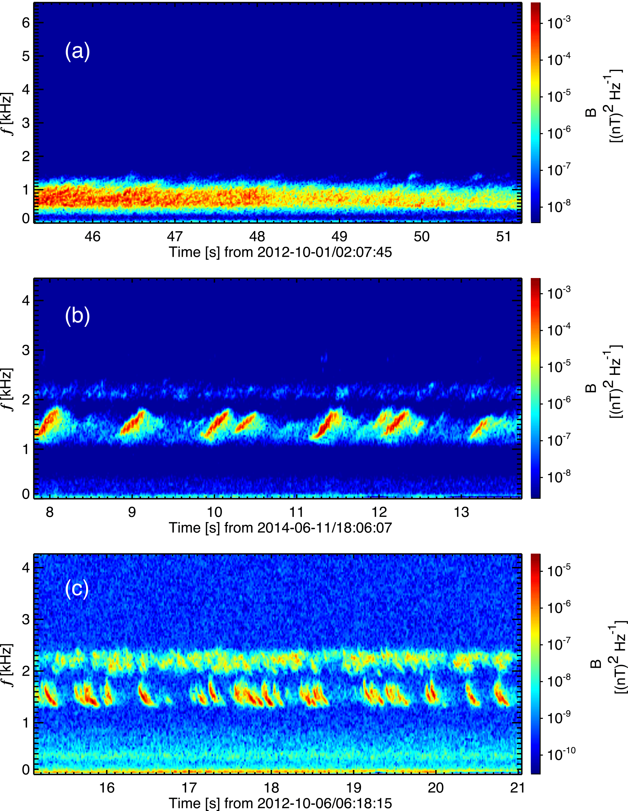
Figure 1Three typical spectrograms of whistler mode electromagnetic emissions with frequency below the electron cyclotron frequency: (a) broadband whistler mode waves, (b) rising-tone chorus, and (c) falling-tone chorus.
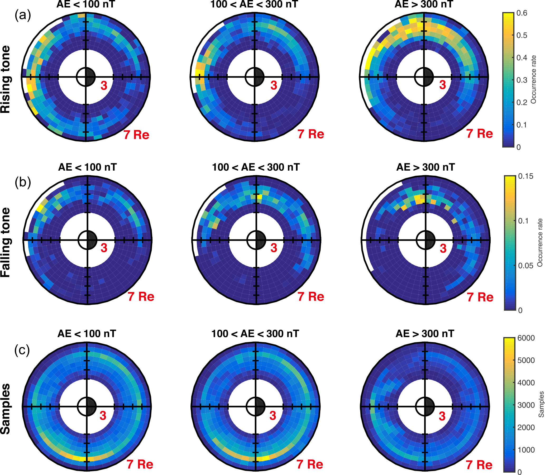
Figure 2Spatial distribution of the occurrence rate of rising-tone (a), falling-tone (b) chorus, and the number of samples (c) in MLT–L coordinates categorized by different AE index.
Figure 1 shows three typical spectrograms of electromagnetic emissions with frequency f<fce, where fce is the electron cyclotron frequency. The upper limit of the y axis in all spectrogram plots in this work is set to fce. These emissions are broadband whistler mode waves (Fig. 1a), rising-tone chorus (Fig. 1b), and falling-tone chorus (Fig. 1c). The term “chorus” in this study specifically means the types of whistler mode emissions shown in Fig. 1b or c, i.e., emissions consisting of discrete elements with frequency chirping. The generation process of frequency chirping chorus waves is believed to be nonlinear (Helliwell, 1967; Katoh and Omura, 2007; Omura et al., 2008; Tao, 2014; Tao et al., 2017b; Vomvoridis et al., 1982). On the contrary, the generation and saturation of broadband whistler mode waves, shown in Fig. 1a, might be understandable using quasi-linear theory (Kennel and Engelmann, 1966; Kennel and Petschek, 1966; Kim et al., 2017; Ossakow et al., 1972; Tao et al., 2017a). By visually inspecting the power spectrogram of each event, we have found 77 216 chorus events in total, including 66 739 rising-tone chorus events and 10 477 falling-tone chorus events. Parameters such as MLT, MLAT (magnetic latitude), and L shell are derived from the TS04D magnetic field model (Tsyganenko and Sitnov, 2005). For 72 events for which TS04D model data are not available, we use the OP77Q (Olson and Pfitzer, 1982) external magnetic field model instead. Considering that most of the events we found are located in the inner magnetosphere with , the mixed use of two magnetic field models does not make a big difference.
The spatial distribution of chorus waves has been studied using data from previous satellite missions such as THEMIS (Li et al., 2009) and Cluster (Meredith et al., 2014). In this section, we present the spatial distribution analysis for rising-tone and falling-tone chorus waves separately using Van Allen Probes data.
Figure 2 presents the distribution of the occurrence rate of rising-tone and falling-tone chorus, and the number of all events under different levels of geomagnetic activity conditions as a function of L and MLT. Both types of chorus waves and samples are sorted into three different levels according to the AE index (auroral electrojet index) (quiet: AE <100 nT, moderate: nT, strong: AE >300 nT), following Meredith et al. (2003). Each bin has a size of 0.5 RE×0.5 MLT. The occurrence rate of chorus is defined as the ratio of the number of chorus wave events to the total number of all events sampled in each bin. As can be seen from the bottom three panels of Fig. 2, the most well sampled region is located from L=5.5 to L=6 and from 14:00 to 20:00 MLT (magnetic local time) during geomagnetically quiet and moderate times, and 11:00 to 18:00 MLT during geomagnetically active times. The fact that the most well sampled region is located at L shells between 5.5 and 6 is not only because of the orbit of the Van Allen Probes, but also the time periods when the continuous-waveform data were collected.
Figure 2 demonstrates that rising-tone and falling-tone chorus waves have different spatial distribution features. From the top three panels of Fig. 2, the highest occurrence rate of rising-tone chorus is located at dawn side and dayside between L=5.5 and 6.5. During quiet and moderate conditions, rising-tone chorus has the highest occurrence rate on the dayside and at L≥5.5. However, during strongly disturbed periods, the largest occurrence rates are seen at the dawn side between 04:00 and 09:00 MLT at . The L shell range covered by the Van Allen Probes data is ; therefore, higher L-shell regions at dayside are not sampled. Note that the waveform data from the EMFISIS onboard the Van Allen probes were not collected randomly, but mostly based on wave amplitudes. Therefore, the statistical results shown in Fig. 2 may have a bias on the larger-amplitude chorus, which potentially reduces the occurrence rate of falling tones, whose amplitudes are typically lower than those of the rising tones (Gao et al., 2014; Li et al., 2011). Furthermore, the present statistical results are very complementary to the previous statistical results based on the THEMIS waveform data (Gao et al., 2014; Li et al., 2011), since THEMIS provides good coverage of chorus wave measurements at L shells over 5–10, compared to the Van Allen Probes coverage over L shells of 3–7.
The distribution of falling-tone chorus is shown in the middle three panels. During quiet time periods (AE<100 nT), falling-tone chorus is distributed almost uniformly across dawn side between , and peaks between 09:00 and 10:00 MLT at . Under moderately disturbed conditions ( nT), falling-tone chorus waves have a higher occurrence rate at dawn side in L shells between 4.5 and 5.5. During strongly disturbed periods, the highest occurrence rate of falling-tone chorus occurs in a narrow MLT range between 05:00 and 07:00 MLT and . Compared with the most intense region for rising-tone chorus (), falling-tone chorus tends to occur at lower L shells () and smaller MLT range for AE>300 nT. Because falling-tone chorus waves tend to be quasi-electrostatic (Li et al., 2011), our result is consistent with that of Li et al. (2016), who found that quasi-electrostatic whistler mode waves preferentially occur at lower L shells compared to quasi-parallel ones. Note that Li et al. (2016) based their analysis on the propagation direction of whistler mode waves only. The physical reason for the preference of quasi-electrostatic whistler mode waves to occur at lower L shell is unknown at this time.
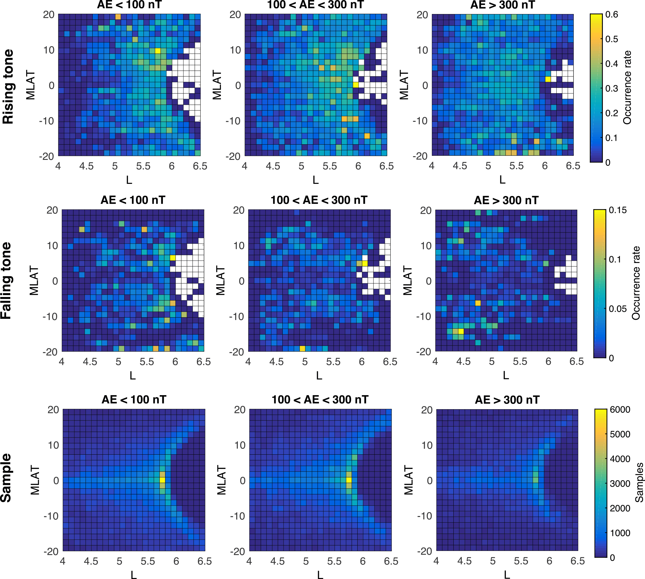
Figure 3 shows the distribution of two types of chorus and the total number of samples in MLAT–L coordinates. The bin size is . The majority of sampled data are located between 5.5 and 6 RE near the equator, typically less than MLAT = 10∘ for any geomagnetic conditions. Top panels show that rising-tone chorus waves have a more uniformly distributed occurrence rate around L=5.5 under all geomagnetic conditions, while falling-tone chorus waves tend to have a higher occurrence rate at higher magnetic latitudes than at the equatorial region at any L shell. This is also consistent with the THEMIS statistical results shown in Li et al. (2011). Further work is needed to understand the different distributions of rising-tone and falling-tone chorus waves.
In this section, we statistically analyze properties of the source region of rising-tone and falling-tone chorus. To reduce the effect of the electron number density on the theoretical estimate of the source-region size (see Sect. 4.2), we exclude 1549 events whose electron number density is larger than 100 cm−3. The electron density is obtained from the Electric Field and Waves density data (Wygant et al., 2013), which was estimated from the spacecraft potential, calibrated from the EMFISIS upper hybrid line. The automatic algorithm described below failed in about 18 % of the events (see Sect. 4.1). In total, there are 54 283 rising-tone chorus events and 7901 falling-tone chorus events used in the following analysis.
4.1 Observation
We statistically determine the source region of chorus using the direction of the Poynting vector with respect to the background magnetic field. The Poynting flux vector P is defined by
where δE and δB are the wave electric field and magnetic field, respectively. One reasonable assumption used in determining the source region of chorus waves or its size along a field line is that inside the source region, there is no preference for the direction of wave excitation with respect to the background magnetic field B. Therefore, waves propagating in both directions should be observed, and the Poynting vector in the source region should have mixed directions with respect to B. Outside the source region, waves propagate away from the generation region and would have a uniform direction of propagation. This assumption has also been used by several previous studies to determine the source region or its size of chorus waves along a magnetic field line in case studies (Hospodarsky et al., 2008; Santolík et al., 2004b). The direction of the background magnetic field is derived from the fluxgate magnetometer (MAG).
Figure 4 shows three events with different types of Poynting fluxes discussed above. The z component of the Poynting flux (hereafter denoted as Pz) of the three events is shown in the second row. The Poynting flux of all chorus elements of event (a) is positive, and that of event (b) is negative. Event (c) shows a case where chorus elements propagate in both directions, suggesting that this event is observed within its generation region. As demonstrated below, when using the Poynting flux to quantitatively estimate the source-region size parallel to the magnetic field, we define a quantity which we call the sign of the event direction, denoted hereafter as S. This quantity takes the value of 1, −1, or 0. If S of an event is 1 (−1), it means that Pz of all chorus elements in the event is positive (negative). On the other hand, if S=0, there are both northward and southward propagating chorus elements in the event.
The value of S for each event is determined automatically in three steps. First, using the spectrogram matrix of the wave magnetic field, we remove background noise and only keep strong wave signals. We define a reference value of the PSD which is the mean value of the maximum five PSDs for waves between 0.1 and 0.8fce, which is the typical frequency range of chorus (Li et al., 2009). Any data points with PSD 3 orders of magnitude lower than the reference PSD will not be considered in the next two steps. Second, we calculate the Poynting flux using the wave magnetic and electric field, and separate the Poynting flux into PzN (Pz>0) and PzS (Pz<0). Here subscripts “N” and “S” refer to northward and southward propagating waves, respectively. The calculated Poynting flux matrix may contain isolated data points that do not belong to any chorus element, which typically consists of continuous data points in the PSD or Pz matrix. To remove these isolated data points, we define a bin to be 0.015 s. This is also the length of the window when performing the moving-window FFT to calculate the PSD spectrogram. Statistical study shows that chorus elements typically last about 0.1–0.8 s (Teng et al., 2017); therefore, a chorus element typically covers a few tens of bins. To consider only data points of chorus elements, we only include bins with more than eight data points and data points that are distributed in three continuous bins. After the first two steps of pre-processing data, the resulting Poynting flux data points are verified to belong to actual chorus elements. These first two steps work correctly for about 82 % of the events previously selected. The remaining 18 % of the events cannot be handled automatically due to too much noise and are therefore excluded from the final data base.
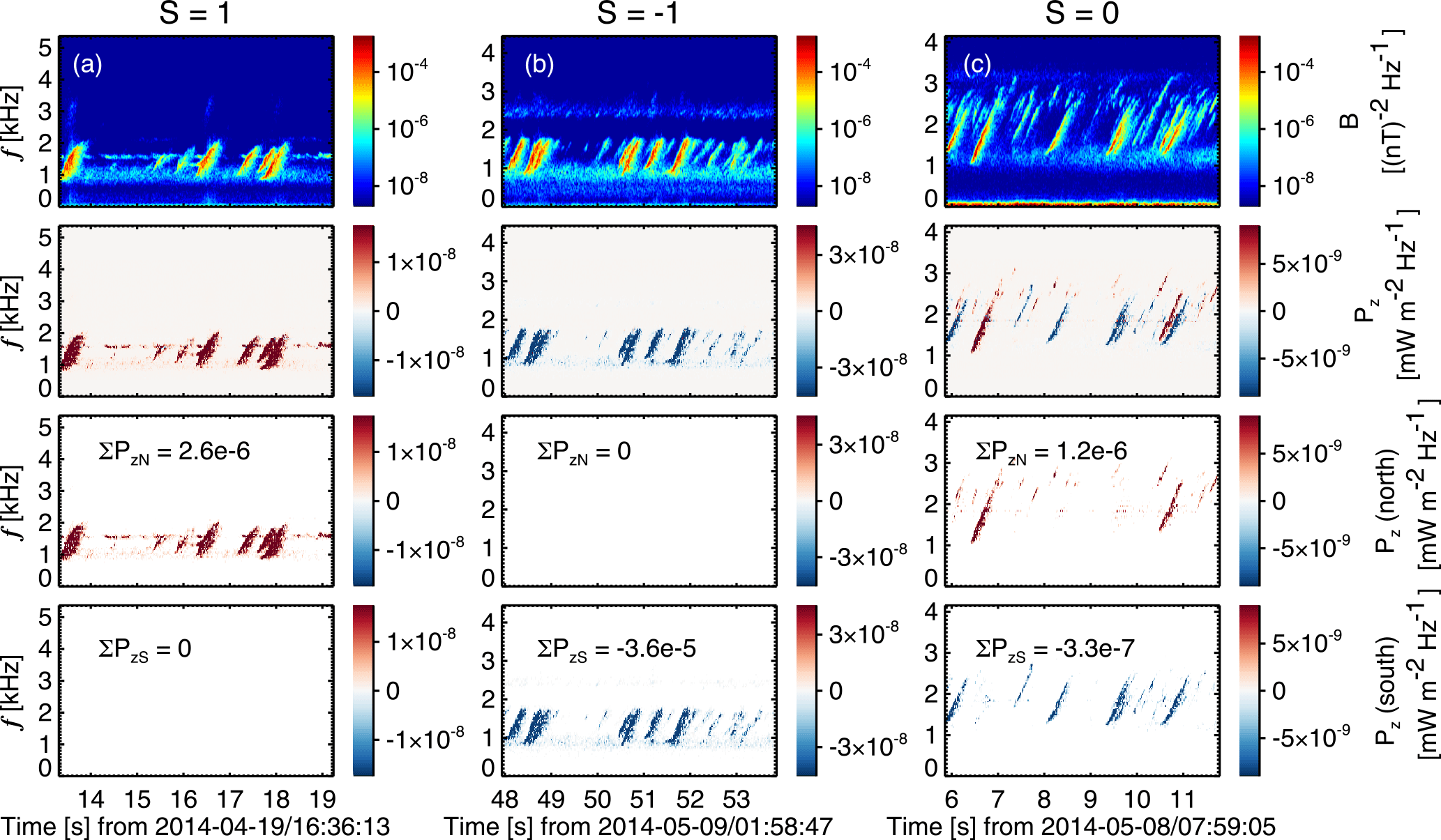
Figure 4Illustration of three types of S: S=1 (a), −1 (b), and 0 (c). From top to bottom rows: the magnetic power spectra density, the z component of the Poynting flux vector (Pz), and the northward and southward ∑Pz.
The third and fourth rows of Fig. 4 show the final Poynting flux matrices for all three events. To determine the value of S for a given event, we calculate the summation of Pz of all selected data points, ∑Pz. Note that , with T=6 s being the average Poynting flux of all waves. If (or ), then S=1 (or −1). In the case when neither ∑PzS nor ∑PzN is 0, the value of S for a given event is determined by
This means that if ∑PzN () is larger than (∑PzN) by 3 orders of magnitude, then S=1 (−1). On the other hand, if the difference between ∑PzN and is within 3 orders of magnitude, it means that waves propagate both northward and southward and therefore S=0. We set the threshold value to be 3 orders of magnitude through experimenting on a subset of the whole database. This process of determining the value of S is illustrated in Fig. 4 for these three types of events.
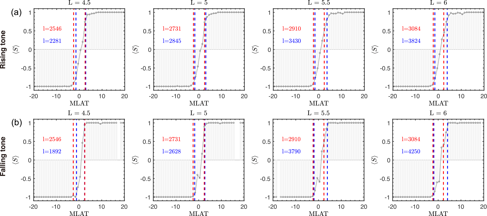
Figure 5Comparison of the source-region size between theoretical (red) and observational results (blue) at different L shell's. The top four panels are for rising-tone chorus, the lower four for falling-tone chorus (for L=4.5 of falling tone, the blue line on the right is overlapping with the red line). Observational estimates of the source-region size are marked by blue dashed lines and theoretical estimates by the red dashed lines. Source-region sizes in kilometers are shown in the corresponding panels.
Figure 5 illustrates the method we use to statistically analyze the source-region size of chorus waves at a given L shell bin with the event direction S defined above. For a bin whose center is at L, we select all events located between L−ΔL and L+ΔL, where ΔL is the width of the bin. We choose ΔL=0.5 in all analyses in this study. Figure 5 displays different L shell's centering at L=4.5, 5, 5.5, and 6 for rising and falling-tone chorus. We uniformly divide the MLAT into 40 bins from −20 to 20∘, so each bin is 1∘ in MLAT. For all events in a given MLAT bin, we then calculate the average value of S, denoted by 〈S〉. A similar quantity has been used by Agapitov et al. (2011b, 2012) to analyze the propagation characteristics of whistler waves. Because of the definition of S, we can re-interpret 〈S〉 as
where N(S=1) is the number of events with S=1, Nt is the total number of events for a given bin, and is the estimated probability of S=1 for that bin. Other variables are defined similarly. Therefore, if 〈S〉=0 for a bin, it means that the probabilities for chorus elements to propagate northward and southward are the same. If 〈S〉=0.9, because 𝒫≥0, this means that at least 90 % of the events in the bin propagate north. Data are represented by gray circles in the selected MLAT bin in Fig. 5. Clearly, for events located in the center of the source region, we expect 〈S〉 to be close to 0. As one moves away from the center of the source region, the absolute value of 〈S〉 increases and eventually becomes 1 as one is completely outside the source region. The top (bottom) four panels of Fig. 5 is 〈S〉 as a function of MLAT for rising-tone (falling-tone) chorus. As can be easily seen, for both types of chorus waves, 〈S〉 is closer to 0 near the equator (MLAT=0), and becomes larger and closer to 1 (−1) as MLAT increases (decreases). Moreover, the sign of S shows that waves propagate northward (southward) in the northern (southern) hemisphere. This confirms previous results of Kurita et al. (2012) that both types of chorus waves are generated near the equator, despite their different characteristics.
Ideally, to obtain the source-region size l, one would use to define the boundary of the source region and estimate l. However, as can be seen from Fig. 5, as , where λ is MLAT. Correspondingly, a small change in can lead to a very large variation in the source-region size. Accordingly, the method we use here is to estimate three boundary sizes determined using , , and , and use the average of three ls to represent the final boundary size. The average of three estimates of l is used to reduce the statistical variation. The source-region sizes for the four L are shown in Fig. 5 and marked by blue dashed lines. The size of the source region is also expressed in kilometers, which is converted from MLAT assuming a dipole field. From these figures, we conclude that the source region of chorus is located within about 3∘ in MLAT for all four Ls for both types of chorus waves. Note that the actual source region of chorus waves for a given event might be time dependent, and could move rapidly around the equator as suggested by previous studies (Inan et al., 2004; Santolik et al., 2004a; Santolík et al., 2004b, 2005). The local minimum of the background magnetic field displacement could also affect the location of the generation region location (Kozelov et al., 2008; Santolik et al., 2004a). These effects should be best investigated using simultaneous observations from multiple spacecraft. Since the current study is superposing a large number of single-point measurements, the size of the source region defined here cannot eliminate the above two effects. Therefore, our way of statistically estimating the source-region size should be interpreted to be the lowest order estimate, and the resulting l might be different from the actual source-region size for a particular event.
4.2 Comparison between the theoretical source-region size and observation
In this section, we compare the source-region size from observation with previous theoretical estimates. Helliwell (1967) estimated that the length of the resonance region parallel to the magnetic field region is roughly
Here β is the inhomogeneity factor, resulting from approximating the magnetic field strength as a function of s using a parabolic function near the equator, i.e., with B0 being the magnetic field strength at s=0. For a dipole field, , where Rp is the planet radius. The cyclotron resonance frequency at the equator . The cyclotron resonant velocity at the equator is
where ωpe is the plasma frequency, and ω is wave frequency. The physical meaning of is essentially the distance for the wave particle interaction phase angle to be changed by π from the equator. Based on the same principle, the source-region size estimated by Trakhtengerts (1995) is
Therefore lT and lH have the same dependence on the electron number density, L shell, and planet radius Rp. Choosing a characteristic frequency of chorus ω=0.3Ω0, . The estimates in Eqs. (4) and (6) should be considered as the lowest order approximation instead of a rigorous theoretical calculation (Helliwell, 1967; Trakhtengerts, 1995). In the analysis below, we only use lH as the theoretical estimate for simplicity.
Before we compare lH with l, we show the dependence of lH on L shell and other parameters. Substituting v‖ (Eq. 5) and β into Eq. (4) results in
For a given ω∕Ω0,
It is clear that lH has a very weak dependence on ne. The value of ne for chorus wave events used in the source region analysis are all below 100 cm−3. In the following analysis, we use a typical electron number density outside the plasmapause ne=10 cm−3. For a given planet such as Earth, Eq. (8) suggests that the source-region size increases with increasing L as L2∕3. Physically, this conclusion can also be understood using Eq. (4). The inhomogeneity factor β decreases with increasing L as . The background magnetic field becomes more homogeneous as L increases, and correspondingly the source-region size increases.
To estimate lH, we use a representative frequency ω=0.3Ω0. The theoretical source-region size is shown by red dashed lines in Fig. 5. For simplicity, the boundary of theoretical source-region size in MLAT is determined from lH, assuming a dipole field and a north–south symmetric source region. For both rising-tone and falling-tone chorus at all four L shell's, lH agrees with l within a factor of 2. Given the crude simplification of the theory, and the statistical nature of our analysis, we conclude that the theoretical estimate roughly agrees with observation. Note here that we do not compare the observed source-region size with that of Omura et al. (2009), because the source-region size of Omura et al. (2009) depends on the wave amplitude δB, which can vary significantly during propagation.
Observations of chorus at other planets should be helpful to further test previous theoretical estimates of chorus source-region size. For example, the radius of Saturn is roughly 10 times larger than that of Earth. At a given L shell, the source-region size of chorus at Saturn should be larger than that at Earth by roughly about a factor of , following Eq. (8). Similar conclusions can be reached for Jupiter. However, these tests depend on the accumulation of enough observational data of chorus waves at these planets.
In this work, we statistically analyzed the distribution and the source-region size parallel to the background magnetic field of rising-tone and falling-tone chorus waves using burst-mode waveform data from the Van Allen Probes. A total of 77 216 rising and falling-tone chorus events were identified visually. Our analysis shows that the spatial distribution of the occurrence rate of rising and falling-tone chorus during periods of different geomagnetic activities is different. Rising-tone chorus waves mainly occur at the dayside sector during quiet times and move to dawn side during active conditions. Falling-tone chorus is more likely to be observed at lower L shells, while rising-tone chorus has a high occurrence rate at larger L shells. The feature is consistent with the recent finding that the quasi-electrostatic whistler mode waves preferentially occur at lower L shells compared to the quasi-parallel ones (Li et al., 2016). In addition, falling-tone chorus tends to have a higher occurrence rate at higher magnetic latitudes than at the equator, whereas rising-tone chorus has a more uniform occurrence rate between the equator and higher latitudes (10∘).
We then investigated the source-region size parallel to the background magnetic field for both types of chorus waves using the direction of the Poynting flux vector. Our results suggest that both types of chorus waves are generated near the equator, despite their different characteristics. This conclusion confirms previous results by Kurita et al. (2012). We showed that statistically the source region of both types of chorus waves is within about 3∘ in MLAT. We also demonstrated that previous theoretical estimates of the source-region size by Helliwell (1967) and Trakhtengerts (1995) roughly agree with observation, and the difference is within about a factor of 2. Our work should be helpful to further understand the generation mechanism of chorus.
The EMFISIS data were obtained from the website (http://emfisis.physics.uiowa.edu/Flight/).
The authors declare that they have no conflict of interest.
This work was supported by NSFC grants 41631071, 41474142, and 41674174. We
acknowledge the NASA Van Allen Probes mission and Craig Kletzing for the use
of the data.
The topical editor, Vincent
Maget, thanks two anonymous
referees for help in evaluating this paper.
Agapitov, O., Krasnoselskikh, V., Dudok de Wit, T., Khotyaintsev, Y., Pickett, J. S., Santolík, O., and Rolland, G.: Multispacecraft observations of chorus emissions as a tool for the plasma density fluctuations' remote sensing, J. Geophys. Res.-Space, 116, A09222, https://doi.org/10.1029/2011JA016540, 2011a. a
Agapitov, O., Krasnoselskikh, V., Khotyaintsev, Y. V., and Rolland, G.: A statistical study of the propagation characteristics of whistler waves observed by Cluster, Geophys. Res. Lett., 38, L20103, https://doi.org/10.1029/2011GL049597, 2011b. a
Agapitov, O., Krasnoselskikh, V., Khotyaintsev, Y. V., and Rolland, G.: Correction to “A statistical study of the propagation characteristics of whistler waves observed by Cluster”, Geophys. Res. Lett., 39, L24102, https://doi.org/10.1029/2012GL054320, 2012. a
Agapitov, O., Blum, L., Mozer, F., Bonnell, J., and Wygant, J.: Chorus whistler wave source scales as determined from multipoint Van Allen Probe measurements, Geophys. Res. Lett., 44, 2634–2642, https://doi.org/10.1002/2017GL072701, 2017. a
Albert, J. M.: Nonlinear interaction of outer zone electrons with VLF waves, Geophys. Res. Lett., 29, 1275, https://doi.org/10.1029/2001GL013941, 2002. a
Albert, J. M. and Young, S. L.: Multidimensional quasi-linear diffusion of radiation belt electrons, Geophys. Res. Lett., 32, L14110, https://doi.org/10.1029/2005GL023191, 2005. a
Bortnik, J., Thorne, R. M., and Inan, U. S.: Nonlinear interaction of energetic electrons with large amplitude chorus, Geophys. Res. Lett., 35, L21102, https://doi.org/10.1029/2008GL035500, 2008. a
Breneman, A. W., Kletzing, C. A., Pickett, J., Chum, J., and Santoík, O.: Statistics of multispacecraft observations of chorus dispersion and source location, J. Geophys. Res., 114, A06202, https://doi.org/10.1029/2008JA013549, 2009. a
Burtis, W. and Helliwell, R.: Banded chorus-A new type of VLF radiation observed in the magnetosphere by OGO 1 and OGO 3, J. Geophys. Res., 74, 3002–3010, https://doi.org/10.1029/JA074i011p03002, 1969. a
Burtis, W. J. and Helliwell, R. A.: Magnetospheric chorus: Occurrence patterns and normalized frequency, Planet. Space Sci., 24, 1007–1010, https://doi.org/10.1016/0032-0633(76)90119-7, 1976. a
Burton, R. K. and Holzer, R. E.: The origin and propagation of chorus in the outer magnetosphere, J. Geophys. Res., 79, 1014–1023, https://doi.org/10.1029/JA079i007p01014, 1974. a
Cornilleau-Wehrlin, N., Etcheto, J., and Burton, R.: Detailed analysis of magnetospheric ELF chorus: Preliminary results, J. Atmos. Sol.-Terr. Phy., 38, 1201–1210, https://doi.org/10.1016/0021-9169(76)90052-0, 1976. a
Gao, X., Li, W., Thorne, R. M., Bortnik, J., Angelopoulos, V., Lu, Q., Tao, X., and Wang, S.: Statistical results describing the bandwidth and coherence coefficient of whistler mode waves using THEMIS waveform data, J. Geophys. Res.-Space, 119, 8992–9003, https://doi.org/10.1002/2014JA020158, 2014. a, b
Gary, S.: Theory of Space Plasma Microinstabilities, Cambridge University Press, New York, 1993. a
Gary, S. P. and Wang, J.: Whistler instability: Electron anisotropy upper bound, J. Geophys. Res., 101, 10749–10754, https://doi.org/10.1029/96JA00323, 1996. a
Helliwell, R. A.: Whistlers and Related Ionospheric Phenomena, Stanford University Press, Stanford, California, 1965. a
Helliwell, R. A.: A theory of discrete VLF emissions from the magnetosphere, J. Geophys. Res., 72, 4773–4790, https://doi.org/10.1029/JZ072i019p04773, 1967. a, b, c, d, e, f
Hikishima, M., Omura, Y., and Summers, D.: Microburst precipitation of energetic electrons associated with chorus wave generation, Geophys. Res. Lett., 37, L07103, https://doi.org/10.1029/2010GL042678, 2010. a
Horne, R. B. and Thorne, R. M.: Potential waves for relativistic electron scattering and stochastic acceleration during magnetic storms, Geophys. Res. Lett., 25, 3011–3014, https://doi.org/10.1029/98GL01002, 1998. a
Horne, R. B., Thorne, R. M., Glauert, S. A., Albert, J. M., Meredith, N. P., and Anderson, R. R.: Timescale for radiation belt electron acceleration by whistler mode chorus waves, J. Geophys. Res., 110, A03225, https://doi.org/10.1029/2004JA010811, 2005a. a
Horne, R. B., Thorne, R. M., Shprits, Y. Y., Meredith, N. P., Glauert, S. A., Smith, A. J., Kanekal, S. G., Baker, D. N., Engebretson, M. J., Posch, J. L., Spasojevic, M., Inan, U. S., Pickett, J. S., and Decreau, P. M. E.: Wave acceleration of electrons in the Van Allen radiation belts, Nature, 437, 227 pp., https://doi.org/10.1038/nature03939, 2005b. a
Hospodarsky, G. B., Averkamp, T. F., Kurth, W. S., Gurnett, D. A., Menietti, J. D., Santoík, O., and Dougherty, M. K.: Observations of chorus at Saturn using the Cassini Radio and Plasma Wave Science instrument, J. Geophys. Res., 113, A12206, https://doi.org/10.1029/2008JA013237, 2008. a
Inan, U. S., Platino, M., Bell, T. F., Gurnett, D. A., and Pickett, J. S.: Cluster measurements of rapidly moving sources of ELF/VLF chorus, J. Geophys. Res., 109, A05214, https://doi.org/10.1029/2003JA010289, 2004. a
Katoh, Y. and Omura, Y.: Computer simulation of chorus wave generation in the Earth's inner magnetosphere, Geophys. Res. Lett., 34, L03102, https://doi.org/10.1029/2006GL028594, 2007. a
Katoh, Y. and Omura, Y.: Effect of the background magnetic field inhomogeneity on generation processes of whistler-mode chorus and broadband hiss-like emissions, J. Geophys. Res., 118, 4189–4198, https://doi.org/10.1002/jgra.50395, 2013. a
Keika, K., Spasojevic, M., Li, W., Bortnik, J., Miyoshi, Y., and Angelopoulos, V.: PENGUIn/AGO and THEMIS conjugate observations of whistler mode chorus waves in the dayside uniform zone under steady solar wind and quiet geomagnetic conditions, J. Geophys. Res., 117, A07212, https://doi.org/10.1029/2012JA017708, 2012. a
Kennel, C. F. and Engelmann, F.: Velocity space diffusion from weak plasma turbulence in a magnetic field, Phys. Fluids, 9, https://doi.org/10.1063/1.1761629, 1966. a
Kennel, C. F. and Petschek, H. E.: Limit on stably trapped particle fluxes, J. Geophys. Res., 71, 1–28, https://doi.org/10.1029/JZ071i001p00001, 1966. a
Kersten, K., Cattell, C. A., Breneman, A., Goetz, K., Kellogg, P. J., Wygant, J. R., Wilson III, L. B., Blake, J. B., Looper, M. D., and Roth, I.: Observation of relativistic electron microbursts in conjunction with intense radiation belt whistler-mode waves, Geophys. Res. Lett., 38, L08107, https://doi.org/10.1029/2011GL046810, 2011. a
Kessel, R., Fox, N., and Weiss, M.: The radiation belt storm probes (RBSP) and space weather, Space Sci. Rev., 179, 531–543, https://doi.org/10.1007/s11214-012-9953-6, 2013. a
Kim, H., Hwang, J., Seough, J., and Yoon, P.: Electron temperature anisotropy regulation by whistler instability, J. Geophys. Res.-Space, 122, 4410–4419, https://doi.org/10.1002/2016JA023558, 2017. a
Kletzing, C., Kurth, W., Acuna, M., MacDowall, R., Torbert, R., Averkamp, T., Bodet, D., Bounds, S., Chutter, M., Connerney, J., Crawford, D., Dolan, J. S., Dvorsky, R., Hospodarsky, G. B., Howard, J., Jordanova, V., Johnson, R. A., Kirchner, D. L., Mokrzycki, B., Needell, G., Odom, J., Mark, D., Pfaff, R., Phillips, J. R., Piker, C. W., Remington, S. L., Rowland, D., Santolik, O., Schnurr, R., Sheppard, D., Smith, C. W., Thorne, R. M., and Tyler, J.: The electric and magnetic field instrument suite and integrated science (EMFISIS) on RBSP, in: The Van Allen Probes Mission, Springer, 127–181, https://doi.org/10.1007/s11214-013-9993-6, 2013. a, b
Kozelov, B. V., Demekhov, A. G., Titova, E. E., Trakhtengerts, V. Y., Santolik, O., Macusova, E., Gurnett, D. A., and Pickett, J. S.: Variations in the chorus source location deduced from fluctuations of the ambient magnetic field: Comparison of Cluster data and the backward wave oscillator model, J. Geophys. Res., 113, A06216, https://doi.org/10.1029/2007JA012886, 2008. a
Kurita, S., Misawa, H., Cully, C. M., Contel, O. L., and Angelopoulos, V.: Source location of falling tone chorus, Geophys. Res. Lett., 39, L22102, https://doi.org/10.1029/2012GL053929, 2012. a, b, c, d
LeDocq, M. J., Gurnett, D. A., and Hospodarsky, G. B.: Chorus source locations from VLF Poynting flux measurements with the Polar spacecraft, Geophys. Res. Lett., 25, 4063–4066, https://doi.org/10.1029/1998GL900071, 1998. a
Li, W., Shprits, Y. Y., and Thorne, R. M.: Dynamic evolution of energetic outer zone electrons due to wave-particle interactions during storms, J. Geophys. Res., 112, A10220, https://doi.org/10.1029/2007JA012368, 2007. a
Li, W., Thorne, R. M., Angelopoulos, V., Bortnik, J., Cully, C. M., Ni, B., LeContel, O., Roux, A., Auster, U., and Magnes, W.: Global distribution of whistler-mode chorus waves observed on the THEMIS spacecraft, Geophys. Res. Lett., 36, L09104, https://doi.org/10.1029/2009GL037595, 2009. a, b, c, d
Li, W., Thorne, R. M., Bortnik, J., Shprits, Y. Y., Nishimura, Y., Angelopoulos, V., Chaston, C., Contel, O. L., and Bonnell, J. W.: Typical properties of rising and falling tone chorus waves, Geophys. Res. Lett., 38, L14103, https://doi.org/10.1029/2011GL047925, 2011. a, b, c, d, e, f
Li, W., Santolik, O., Bortnik, J., Thorne, R., Kletzing, C., Kurth, W., and Hospodarsky, G.: New chorus wave properties near the equator from Van Allen Probes wave observations, Geophys. Res. Lett., 43, 4725–4735, https://doi.org/10.1002/2016GL068780, 2016. a, b, c, d
Lorentzen, K. R., Blake, J. B., Inan, U. S., and Bortnik, J.: Observations of relativistic electron microbursts in association with VLF chorus, J. Geophys. Res., 106, 6017–6027, https://doi.org/10.1029/2000JA003018, 2001. a
Mauk, B., Fox, N. J., Kanekal, S., Kessel, R., Sibeck, D., and Ukhorskiy, A.: Science objectives and rationale for the radiation belt storm probes mission, Space Sci. Rev., 179, 3–27, https://doi.org/10.1007/s11214-012-9908-y, 2013. a
Meredith, N. P., Horne, R. B., Thorne, R. M., and Anderson, R. R.: Favored regions for chorus-driven electron acceleration to relativistic energies in the Earth's outer radiation belt, Geophys. Res. Lett., 30, 1871, https://doi.org/10.1029/2003GL017698, 2003. a
Meredith, N. P., Horne, R. B., Li, W., Thorne, R. M., and Sicard-Piet, A.: Global model of low-frequency chorus () from multiple satellite observations, Geophys. Res. Lett., 41, 280–286, https://doi.org/10.1002/2013GL059050, 2014. a, b
Mourenas, D., Artemyev, A. V., Agapitov, O. V., Krasnoselskikh, V., and Mozer, F. S.: Very oblique whistler generation by low-energy electron streams, J. Geophys. Res.-Space, 120, 3665–3683, https://doi.org/10.1002/2015JA021135, 2015. a
Ni, B., Thorne, R. M., Shprits, Y. Y., and Bortnik, J.: Resonant scattering of plasma sheet electrons by whistler-mode chorus: Contribution to diffuse auroral precipitation, Geophys. Res. Lett., 35, L11106, https://doi.org/10.1029/2008GL034032, 2008. a
Ni, B., Thorne, R. M., Meredith, N. P., Horne, R. B., and Shprits, Y. Y.: Resonant scattering of plasma sheet electrons leading to diffuse auroral precipitation: 2. Evaluation for whistler mode chorus waves, J. Geophys. Res., 116, A04219, https://doi.org/10.1029/2010JA016233, 2011. a
Ni, B., Thorne, R. M., Zhang, X., Bortnik, J., Pu, Z., Xie, L., Hu, Z.-j., Han, D., Shi, R., Zhou, C., and Gu, X.: Origins of the Earth's diffuse auroral precipitation, Space Sci. Rev., 200, 205–259, https://doi.org/10.1007/s11214-016-0234-7, 2016. a
Nishimura, Y., Bortnik, J., Li, W., Thorne, R. M., Lyons, L. R., Angelopoulos, V., Mende, S. B., Bonnell, J. W., Contel, O. L., Cully, C., Ergun, R., and Auster, U.: Identifying the driver of pulsating aurora, Science, 330, 81–84, https://doi.org/10.1126/science.1193186, 2010. a
Nishimura, Y., Bortnik, J., Li, W., Thorne, R. M., Ni, B., Lyons, L. R., Angelopoulos, V., Ebihara, Y., Bonnell, J. W., Le Contel, O., and Auster, U.: Structures of dayside whistler-mode waves deduced from conjugate diffuse aurora, J. Geophys. Res., 118, 664–673, https://doi.org/10.1029/2012JA018242, 2013. a
Nunn, D.: A self-consistent theory of triggered VLF emissions, Planet. Space Sci., 22, 349–378, https://doi.org/10.1016/0032-0633(74)90070-1, 1974. a
Nunn, D. and Omura, Y.: A computational and theoretical analysis of falling frequency VLF emissions, J. Geophys. Res., 117, A08228, https://doi.org/10.1029/2012JA017557, 2012. a
Olson, W. and Pfitzer, K. A.: A dynamic model of the magnetospheric magnetic and electric fields for July 29, 1977, J. Geophys. Res.-Space, 87, 5943–5948, https://doi.org/10.1029/JA087iA08p05943, 1982. a
Omura, Y., Katoh, Y., and Summers, D.: Theory and simulation of the generation of whistler-mode chorus, J. Geophys. Res., 113, A04223, https://doi.org/10.1029/2007JA012622, 2008. a, b, c
Omura, Y., Hikishima, M., Katoh, Y., Summers, D., and Yagitani, S.: Nonlinear mechanisms of lower-band and upper-band VLF chorus emissions in the magnetosphere, J. Geophys. Res., 114, A07217, https://doi.org/10.1029/2009JA014206, 2009. a, b
Ossakow, S. L., Ott, E., and Haber, I.: Nonlinear evolution of whistler instabilities, Phys. Fluids, 15, 2314–2326, https://doi.org/10.1063/1.1693875, 1972. a, b
Parrot, M., Santolík, O., Cornilleau-Wehrlin, N., Maksimovic, M., and Harvey, C. C.: Source location of chorus emissions observed by Cluster, Ann. Geophys., 21, 473–480, https://doi.org/10.5194/angeo-21-473-2003, 2003. a
Saito, S., Miyoshi, Y., and Seki, K.: Relativistic electron microbursts associated with whistler chorus rising tone elements: GEMSIS-RBW simulations, J. Geophys. Res., 117, A10206, https://doi.org/10.1029/2012JA018020, 2012. a
Santolík, O. and Gurnett, D. A.: Transverse dimensions of chorus in the source region, Geophys. Res. Lett., 30, 1031, https://doi.org/10.1029/2002GL016178, 2003. a, b
Santolík, O., Gurnett, D. A., and Pickett, J. S.: Multipoint investigation of the source region of storm-time chorus, Ann. Geophys., 22, 2555–2563, https://doi.org/10.5194/angeo-22-2555-2004, 2004a. a, b
Santolík, O., Gurnett, D. A., Pickett, J. S., Parrot, M., and Cornilleau-Wehrlin, N.: A microscopic and nanoscopic view of storm-time chorus on 31 March 2001, Geophys. Res. Lett., 31, L02801, https://doi.org/10.1029/2003GL018757, 2004b. a, b, c
Santolík, O., Gurnett, D., Pickett, J., Parrot, M., and Cornilleau-Wehrlin, N.: Central position of the source region of storm-time chorus, Planet. Space Sci., 53, 299–305, https://doi.org/10.1016/j.pss.2004.09.056, 2005. a
Santolík, O., Gurnett, D. A., Pickett, J. S., Chum, J., and Cornilleau-Wehrlin, N.: Oblique propagation of whistler mode waves in the chorus source region, J. Geophys. Res., 114, A00F03, https://doi.org/10.1029/2009JA014586, 2009. a
Soto-Chavez, A. R., Wang, G., Bhattacharjee, A., Fu, G. Y., and Smith, H. M.: A model for falling-tone chorus, Geophys. Res. Lett., 41, 1838–1845, https://doi.org/10.1002/2014GL059320, 2014. a
Spasojevic, M. and Inan, U. S.: Drivers of chorus in the outer dayside magnetosphere, J. Geophys. Res., 115, A00F09, https://doi.org/10.1029/2009JA014452, 2010. a
Sudan, R. N. and Ott, E.: Theory of triggered VLF emissions, J. Geophys. Res., 76, 4463–4476, https://doi.org/10.1029/JA076i019p04463, 1971. a
Summers, D., Thorne, R. M., and Xiao, F.: Relativistic theory of wave-particle resonant diffusion with application to electron acceleration in the magnetosphere, J. Geophys. Res., 103, 20487–20500, https://doi.org/10.1029/98JA01740, 1998. a
Tao, X.: A numerical study of chorus generation and the related variation of wave intensity using the DAWN code, J. Geophys. Res.-Space, 119, 3362–3372, https://doi.org/10.1002/2014JA019820, 2014. a, b
Tao, X., Chan, A. A., Albert, J. M., and Miller, J. A.: Stochastic modeling of multidimensional diffusion in the radiation belts, J. Geophys. Res., 113, A07212, https://doi.org/10.1029/2007JA012985, 2008. a
Tao, X., Thorne, R. M., Li, W., Ni, B., Meredith, N. P., and Horne, R. B.: Evolution of electron pitch-angle distributions following injection from the plasma sheet, J. Geophys. Res., 116, A04229, https://doi.org/10.1029/2010JA016245, 2011. a
Tao, X., Bortnik, J., Thorne, R. M., Albert, J., and Li, W.: Effects of amplitude modulation on nonlinear interactions between electrons and chorus waves, Geophys. Res. Lett., 39, L06102, https://doi.org/10.1029/2012GL051202, 2012. a
Tao, X., Bortnik, J., Albert, J. M., Thorne, R. M., and Li, W.: The importance of amplitude modulation in nonlinear interactions between electrons and large amplitude whistler waves, J. Atmos. Sol.-Terr. Phys., 99, 67–72, https://doi.org/10.1016/j.jastp.2012.05.012, 2013. a
Tao, X., Bortnik, J., Albert, J. M., Thorne, R. M., and Li, W.: Effects of discreteness of chorus waves on quasilinear diffusion-based modeling of energetic electron dynamics, J. Geophys. Res.-Space, 119, 8848–8857, https://doi.org/10.1002/2014JA020022, 2014a. a
Tao, X., Lu, Q., Wang, S., and Dai, L.: Effects of magnetic field configuration on the day-night asymmetry of chorus occurrence rate: A numerical study, Geophys. Res. Lett., 41, 6577–6582, https://doi.org/10.1002/2014GL061493, 2014b. a
Tao, X., Chen, L., Liu, X., Lu, Q., and Wang, S.: Quasilinear analysis of saturation properties of broadband whistler mode waves, Geophys. Res. Lett., 44, 8122–8129, https://doi.org/10.1002/2017GL074881, 2017a. a, b
Tao, X., Zonca, F., and Chen, L.: Identify the nonlinear wave-particle interaction regime in rising tone chorus generation, Geophys. Res. Lett., 44, 3441–3446, https://doi.org/10.1002/2017GL072624, 2017b. a, b
Tao, X., Zonca, F., and Chen, L.: Investigations of the electron phase space dynamics in triggered whistler wave emissions using low noise δf method, P. S. IAEA, 59, 094001, https://doi.org/10.1088/1361-6587/aa759a, 2017c. a
Taubenschuss, U., Khotyaintsev, Y. V., Santolík, O., Vaivads, A., Cully, C. M., Contel, O. L., and Angelopoulos, V.: Wave normal angles of whistler mode chorus rising and falling tones, J. Geophys. Res.-Space, 119, 9567–9578, https://doi.org/10.1002/2014JA020575, 2014. a
Teng, S., Tao, X., Xie, Y., Zonca, F., Chen, L., Fang, W., and Wang, S.: Analysis of the Duration of Rising Tone Chorus Elements, Geophys. Res. Lett., 44, 12074–12082, https://doi.org/10.1002/2017GL075824, 2017. a
Thorne, R. M., Ni, B., Tao, X., Horne, R. B., and Meredith, N. P.: Scattering by chorus waves as the dominant cause of diffuse auroral precipitation, Nature, 467, 943–946, https://doi.org/10.1038/nature09467, 2010. a, b
Thorne, R. M., Li, W., Ni, B., Ma, Q., Bortnik, J., Chen, L., Baker, D. N., Spence, H. E., Reeves, G. D., Henderson, M. G., Kletzing, C. A., Kurth, W. S., Hospodarsky, G. B., Blake, J. B., Fennell, J. F., Claudepierre, S. G., and Kanekal, S. G.: Rapid local acceleration of relativistic radiation-belt electrons by magnetospheric chorus, Nature, 504, 411–414, https://doi.org/10.1038/nature12889, 2013. a
Trakhtengerts, V. Y.: Magnetosphere cyclotron maser: Backward wave oscillator generation regime, J. Geophys. Res., 100, 17205–17210, https://doi.org/10.1029/95JA00843, 1995. a, b, c, d, e
Tsurutani, B. T., Lakhina, G. S., and Verkhoglyadova, O. P.: Energetic electron (>10 keV) microburst precipitation, ∼ 5–15 s X-ray pulsations, chorus, and wave-particle interactions: A review, J. Geophys. Res.-Space, 118, 2296–2312, https://doi.org/10.1002/jgra.50264, 2013. a
Tsyganenko, N. and Sitnov, M.: Modeling the dynamics of the inner magnetosphere during strong geomagnetic storms, J. Geophys. Res, 110, A03208, https://doi.org/10.1029/2004JA010798, 2005. a
Viñas, A. F., Moya, P. S., Navarro, R. E., Valdivia, J. A., Araneda, J. A., and Muñoz, V.: Electromagnetic fluctuations of the whistler-cyclotron and firehose instabilities in a Maxwellian and Tsallis-kappa-like plasma, J. Geophys. Res.-Space, 120, 3307–3317, https://doi.org/10.1002/2014JA020554, 2015. a
Vomvoridis, J. L., Crystal, T. L., and Denavit, J.: Theory and computer simulations of magnetospheric very low frequency emissions, J. Geophys. Res., 87, 1473–1489, https://doi.org/10.1029/JA087iA03p01473, 1982. a, b, c
Wygant, J., Bonnell, J., Goetz, K., Ergun, R., Mozer, F., Bale, S., Ludlam, M., Turin, P., Harvey, P., Hochmann, R., Harps, K., Dalton, G., McCauley, J., Rachelson, W., and Gordon, D.: The Electric Field and Waves Instruments on the Radiation Belt Storm Probes Mission, Space Sci. Rev., 179, 183–220, https://doi.org/10.1007/s11214-013-0013-7, 2013. a
Yoon, P. H.: Large-amplitude whistler waves and electron acceleration, Geophys. Res. Lett., 38, L12105, https://doi.org/10.1029/2011GL047893, 2011. a