Determination of gravity wave parameters in the airglow combining photometer and imager data

Mesospheric airglow measurements of two or three layers were used to characterize both vertical and horizontal parameters of gravity waves. The data set was acquired coincidentally from a multi-channel filter (Multi-3) photometer and an all-sky imager located at São João do Cariri (7.4^∘ S, 36.5^∘ W) in the equatorial region from 2001 to 2007. Using a least-square fitting and wavelet analysis technique, the phase and amplitude of each observed wave were determined, as well as the amplitude growth. Using the dispersion relation of gravity waves, the vertical and horizontal wavelengths were estimated and compared to the horizontal wavelength obtained from the keogram analysis of the images observed by an all-sky imager. The results show that both horizontal and vertical wavelengths, obtained from the dispersion relation and keogram analysis, agree very well for the waves observed on the nights of 14 October and 18 December 2006. The determined parameters showed that the observed wave on the night of 18 December 2006 had a period of $\sim \mathrm{43.8}\pm \mathrm{2.19}$ min, with the horizontal wavelength of 235.66 ± 11.78 km having a downward phase propagation, whereas that of 14 October 2006 propagated with a period of $\sim \mathrm{36.00}\pm \mathrm{1.80}$ min with a horizontal wavelength of $\sim \mathrm{195}\pm \mathrm{9.80}$ km, and with an upward phase propagation. The observation of a wave taken by a photometer and an all-sky imager allowed us to conclude that the same wave could be observed by both instruments, permitting the investigation of the two-dimensional wave parameter.

Keywords. Atmospheric composition and structure (airglow and aurora) – electromagnetics (wave propagation) – history of geophysics (atmospheric sciences)

1 Introduction

Propagation of atmospheric gravity waves in the upper atmosphere is extremely unstable. The vertical component of the propagating gravity wave is a very vital aspect in investigating the coupling dynamics between different regions of the atmosphere (Hocking, 1996). Due to the exponential decay of density with altitude and conservation of energy, gravity wave amplitudes increase exponentially with altitude, whereas dissipation processes like wave saturation and wave interaction with other waves and background wind limit the growth of the amplitude of the wave (Fritts and Alexander, 2003). Some studies on gravity wave saturations revealed that the momentum is transferred into the background wind, thereby depositing the wave energy into the background atmosphere (e.g. Fritts, 1984; Smith et al., 1987; Dewan and Good, 1986; Fritts and Alexander, 2003).

Measurements of gravity waves with periodicity in the mesosphere and lower thermosphere (MLT) region require passive airglow observation of the sky in a two-dimensional form with relatively high temporal resolution (in a few minutes). Among several gravity wave observational techniques, such as radio frequency and optical measurements, airglow observations using a photometer and all-sky imagers have been effectively used (Hecht et al., 1987; Taylor et al., 1991, 2009; Takahashi et al., 1992; Taori and Taylor, 2006). Airglow emissions are prominent physical phenomena used to further study the vertical and horizontal parameters of gravity waves. According to Takahashi et al. (2011), the airglow emission layers that have been extensively used to monitor wave activity in the MLT region are OI5577 (hereafter OI), O₂(0–1) band (hereafter O₂), NaD-line (hereafter NaD) and OH(6–2) band (hereafter OH) at their respective peak emission altitudes of 97, 94, 90 and 87 km. Simultaneous observation of multiple airglow emissions is one of the techniques used to investigate the vertical propagation of gravity waves. For this technique to be feasible, the vertical wavelengths of the wave must be larger than the thickness of the airglow emission layer (Ghodpage et al., 2014). According to Noxon (1978) and Taori et al. (2005), such observational data can be used to compute the amplitude growth and the propagation characteristics of gravity waves.

In the present study, we investigated gravity wave parameters propagating vertically through OI, O₂, NaD and OH emissions, their phase difference and variability of the amplitudes of the oscillations. Using the dispersion relation of gravity waves, the horizontal and vertical wavelengths are estimated for the observed short period oscillations (Vadas and Liu, 2009). The discussion will be focused on the similar periodicity observed within the three emission layers; the amplitude growth and the propagation direction.

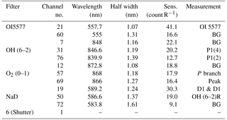
Table 1 Multi-channel airglow photometer (Multi-3) wavelength resolution and sensitivity.

2 Instrumentation and observation

The instruments used for the present study are the multi-channel filter photometer (Multi-3), the all-sky imager and the meteor radar at São João do Cariri, located geographically at 7.4 ^∘ S and 36.5^∘ W. Among the listed instruments, the photometer is the main instrument used in observing the vertical parameters of the waves of interest, whereas the all-sky imager and the meteor radar were co-located instruments used to observe the horizontal parameters and the wind velocity respectively.

2.1 Photometer

A multi-channel tilting filter photometer (Multi-3) with five interference filters was used to measure the OI, O₂, NaD and OH mesospheric airglow emissions. The observations were made between January 2001 and December 2007, resulting in 1051 nights of clear sky. Out of 1051 nights, only 389 nights present similar periods in at least two emission layers, of which 24 nights present similar periods in three emission layers.

The background continuum intensity (R nm⁻¹) and the line intensity (R) were measured in obtaining the zenith sky spectrum by tilting the filters relative to their optical axes in which a scan of about 8 nm wavelength was made. The mesospheric component of the OI557.7 nm was estimated by subtracting the ionospheric F region component computed as 20 % of the simultaneously observed OI630.0 nm intensity (Silverman, 1970). The time interval between the observation cycle was approximately 2 min, thereby making the temporal resolution 2 min. The photometer characteristics, spectral resolution and sensitivity, are summarised in Table 1.

A MgO white screen illuminated by a laboratory standard lamp (Eppley 8315, 100 W Tungsten filament lamp) was used to calibrate the absolute sensitivity (counts/Rayleigh) of the photometer. The estimated error in the absolute intensity for OI was approximately 5 and 10 % for OH(6–2) and O₂ due to the increased systematic error in calibration. For rotational temperature (TOH), the instrumental error determined was ±3 K (Takahashi et al., 1998).

The usual observation scheme was undertaken with a period of 13 nights per month focused around the time of new moon with more than 6 h of uninterrupted observation time per night. In this work, a database of OI, O₂, NaD and OH was analysed to find the similar periodicities in the propagating gravity waves in each emission altitude. More details on the multi-channel filter photometer can be found in Kirchhoff (1984), Buriti et al. (2001, 2004), and Wrasse et al. (2004).

2.2 All-sky imager

An all-sky imager in São João do Cariri was used. Images of OH (Meinel), OI5577, OI6300 and OI7774 airglow emission layers were taken by this equipment. With regards to the present work, only the OH Meinel airglow image corresponding to the selected coincident photometer observation was used.

The airglow all-sky imager is an optical instrument made of a fast fish-eye (f∕4) lens and a telecentric lens system, a filter wheel, a charged coupled device (CCD) camera, and a set of lenses for reconstruction of the images on the CCD. The entire system is microcomputer-based controlled. The CCD camera has an area of 6.04 cm², with a 1024 × 1024 back-illuminated pixel array of 14 bits per pixel. In order to enhance the signal-to-noise ratio, the images were binned on-chip down to a resolution of 512 × 512. The high quantum efficiency, low dark noise (0.5 electrons pixel⁻¹ s⁻¹), low readout noise (15 electron rms) and high linearity (0.05 %) of this device enable it to measure airglow emissions (Medeiros et al., 2001). More details about the São João do Cariri imager have been reported by Medeiros et al. (2005).

2.3 Meteor radar

A SKiYMET all-sky interferometric meteor radar using an antenna array composed of two-element reception yagi antennas and three-element transmitting yagi antenna (five antennas) was used to observe winds in the mesosphere. This radar operates at a frequency of 35.24 MHz with a maximum output power of 12 kW. The radar measures the radial velocity by transmitted radiation scattered from meteor trails and the differences in the phase of the signal received by each possible pairing of antennas determines the position of the trail. This radar also measures the temperature at the height of the meteor peak count rates, but this parameter was not used in this work. The range is obtained by the delay between the transmitted and received signal. The least-square fitting technique applied to all the radial velocities measured in a given time/height bin was used to determine the zonal, meridional and vertical velocity components. Vertical velocities are normally very small and are therefore ignored. The respective temporal and vertical resolutions of this radar are typically 60 min and 2–3 km. More details on the radar have been published elsewhere (Hocking, 1996, 2001; Buriti et al., 2008).

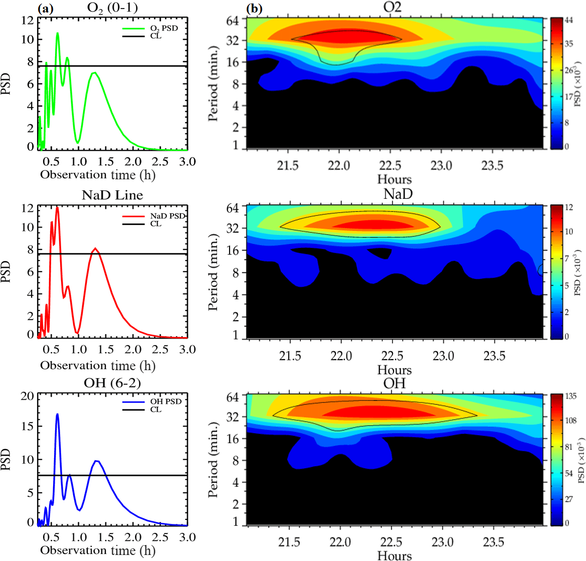
Figure 1 (a) Lomb–Scargle periodogram and (b) wavelet spectrogram for the airglow intensity on 14 October 2006. The blue line is for the OH emission, the red line is for NaD emission and the black line is for O₂.

2.4 Methodology and data analysis

2.4.1 Photometer time series

The first step considered before processing the photometer time series data was the background intensity variation. This variation gives the degree of contaminants composed of artificial light sources, clouds or astronomical lights. The time range with high contaminants is eliminated, which leads to the reduction of the time duration of the observation period.

Secondly, high-frequency oscillations are removed by taking three-point running means. Since gravity waves are modulated by tidal waves (Preusse et al., 2008; Takahashi et al., 1999), the effects of tides are eliminated by constructing a harmonics for ter-diurnal and semi-diurnal tides. The harmonics (H) used is expressed mathematically by

$$\begin{array}{}\text{(1)}& H=A+B\cos \left({\displaystyle \frac{\mathrm{2}\mathit{\pi }(x-\mathit{\varphi })}{T}}\right)+C\cos \left({\displaystyle \frac{\mathrm{2}\mathit{\pi }(x-\mathit{\varphi })}{T}}\right),\end{array}$$

where A, B and C are the unknown amplitude, x is the time of observation, ϕ is the phase and T is the period. Subtracting the harmonics from the average (smoothed) intensity, the residual (only gravity waves) time series is obtained. The residual is then subjected to a Lomb–Scargle periodogram and wavelet spectrogram to obtain the observed gravity wave period. Using the least-square fitting method and the wavelet spectrogram, the amplitude and the phase were estimated. The vertical phase velocity (V_z) was then estimated from the quotient of the difference between the higher and lower emission layers observed and their corresponding phase, expressed by Eq. (2):

$$\begin{array}{}\text{(2)}& V_z={\displaystyle \frac{\mathrm{\Delta }\mathrm{d}}{\mathrm{\Delta }\mathit{\varphi }}}.\end{array}$$

Multiplying the period obtained by the vertical phase speed, the vertical wavelength was obtained using Eq. (3).

$$\begin{array}{}\text{(3)}& {\mathit{\lambda }}_z=V_z\times T\end{array}$$

Using the intrinsic period, the horizontal wavelength was calculated by using the dispersion relation for gravity waves (Gossard and Hooke, 1975),

$$\begin{array}{}\text{(4)}& k_H=\left[\right(m^{\mathrm{2}}+{\displaystyle \frac{\mathrm{1}}{\mathrm{4}{H}^{\mathrm{2}}}}){\mathit{\omega }}_I^{\mathrm{2}}\times (N^{\mathrm{2}}-{\mathit{\omega }}_I^{\mathrm{2}}{)}^{-\mathrm{1}}{]}^{\frac{\mathrm{1}}{\mathrm{2}}},\end{array}$$

where m is the vertical wavenumber, H is the scale height, N is the buoyancy frequency and ω_I is the intrinsic frequency. By scale analysis, the effect of the Coriolis parameter is ignored due to the period of observation and the location of the observation site. From the horizontal wavenumber, k_H, the horizontal wavelength is estimated using Eq. (5),

$$\begin{array}{}\text{(5)}& {\mathit{\lambda }}_H={\displaystyle \frac{\mathrm{2}\mathit{\pi }}{k_H}}.\end{array}$$

The intrinsic frequency, ω_I, was estimated by finding the difference between the vertical observed period obtained from Lomb–Scargle and the estimated background wind frequency using Eq. (6).

$$\begin{array}{}\text{(6)}& {\mathit{\omega }}_I={\mathit{\omega }}_{\mathrm{0}}-U_H\cdot k_H\end{array}$$

where ω_I is the intrinsic frequency, ω₀ is the observed frequency, U_H is the velocity of the background wind and k_H is the horizontal wavenumber estimated from the horizontal wavelength obtained from the keogram analysis.

Figure 2 (a) Same as Fig. 1a but for 18 December 2006.

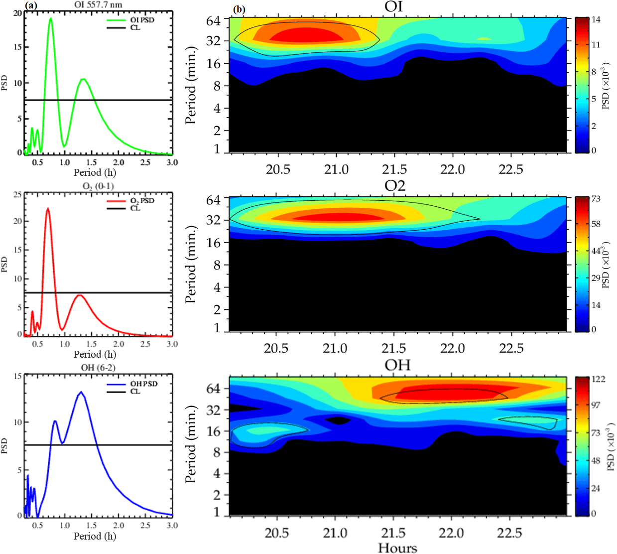
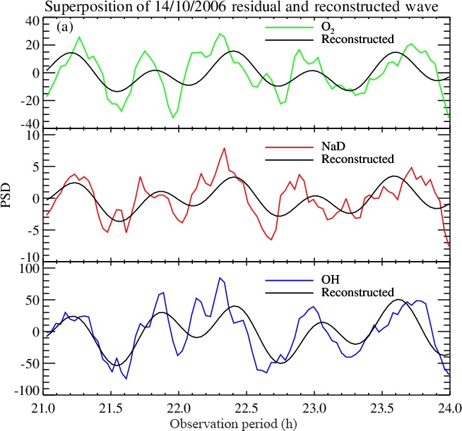
Figure 3 The superposition of the 14 October 2006 residual wave and the reconstructed wave with two harmonics.

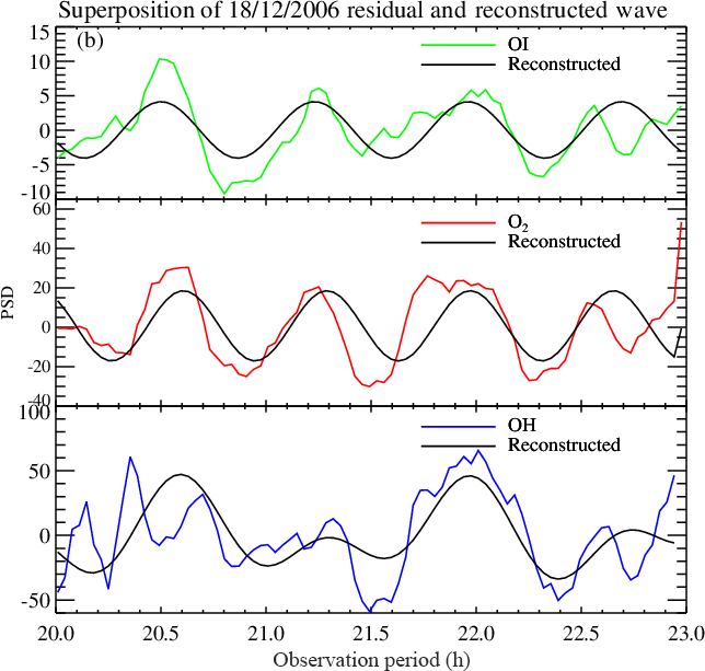
Figure 4 The superposition of the 18 December 2006 residual wave and the reconstructed wave with two harmonics.

2.4.2 All-sky image

The co-located all-sky images were analysed using the keogram analysis from which the horizontal parameters of the same wave are obtained. The keogram simply separates the image of the oscillation under study into meridional and zonal components. The wave parameters are then obtained from the geometrical relationship between the components. For this study we used the keogram analysis to obtain the horizontal wave parameters such as the horizontal wavelength, the period and the direction of propagation of the wave observed by the photometer. Details on the methodology of the keogram analysis can be found in Paulino et al. (2011), with more details in Figueiredo et al. (2018). The co-located meteor radar is operated in a routine base providing information on zonal and meridional wind velocities which aided in the estimation of the intrinsic wave frequency.

3 Results and discussion

3.1 Airglow photometer

Out of the 7 years of data used, we found two nights which present similar periods of oscillations in the airglow emission layers in the photometer data and images from the all-sky imager. Due to cloud contaminations, only 3 h of observed data were used for the selected nights. On 14 October, observations made between 21:00 and 23:00 local time (LT) were used in the present study, whereas on 18 December, observations between 20:00 and 22:00 LT were used. Similar periodic oscillations were found in the co-located airglow images and the spectral characteristics of these oscillations were estimated and studied.

The gravity wave period estimated using Lomb–Scargle on the night of 14 October 2006 in the O₂, NaD and OH airglow emission layers presented two major peaks with confidence levels greater than 95 %; Fig. 1a shows the Lomb–Scargle periodogram; the first peak presented a period of ∼ 0.60 ± 0.03 h (36 ± 2.00 min) and ∼ 1.33 ± 0.07 h (79.80 ± 4.00 min) for the second peak. To confirm the true presence of the second peak, we subjected this period to the Horne and Baliunas test (Horne and Baliunas, 1986). According to the Horne and Baliunas test, spectral leaked frequencies may have significant height, which might appear as a true signal. The Horne and Baliunas test is used to test the originality of the frequencies with lower power spectral density (PSD). This was done by subtracting a sinusoid with frequency corresponding to the most significant peak from the data (Ferraz-Mello, 1981) and recomputing the periodogram. If the second peak (the so-called ghost frequency) still exists, it implies the second peak is a true signal. The Horne and Baliunas test was done to verify the true existence of the periodicities obtained in the Lomb–Scargle periodograms (Fig. 1a) for the cases presented, but the test plots are not shown here. Since the photometer data is almost evenly distributed, wavelet analysis (Torrence and Compo, 1998) (as shown in Fig. 1b) of the same residual data was applied to confirm the periods observed in the Lomb–Scargle analysis. Comparing these two techniques, we affirm that the periods are true.

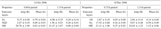
Table 2 The estimated amplitude and phase of 14 October and 18 December 2006 observed waves.

Similarly, Fig. 2a and b show the same analysis for the waves observed on 18 December 2006. It is noted that, for the OI and O₂ emission layers, the oscillation periods of ∼ 0.73 ± 0.04 (43.80 ± 2.20 min) and ∼ 1.33 ± 0.10 h (79.80 ± 4.00 min) were obtained in which the highest peak was ∼ 0.73 ± 0.04 h (43.80 ± 2.20 min). On the other hand, the OH emission layer had the highest peak at ∼ 1.33 ± 0.10 h (79.80 ± 4.00 min) and the lowest at 0.73 ± 0.10 h. Due to this inversion, the 1.33 ± 0.10 h (79.80 ± 4.00 min) period dominated in the wavelet spectrogram, as shown in Fig. 2b, whereas the 0.73 ± 0.10 h period was not seen.

Figure 5 Upward phase propagation of the two harmonics of the 14 October 2006 observed wave.

In order to confirm the result estimated from the residual time, an artificial wave was reconstructed using the amplitude, phase and observed period as presented in Table 3 to evaluate the obtained result. To achieve that, the reconstructed waves of two harmonics were overplotted on the residual photometer data as shown in Figs. 3 and 4.

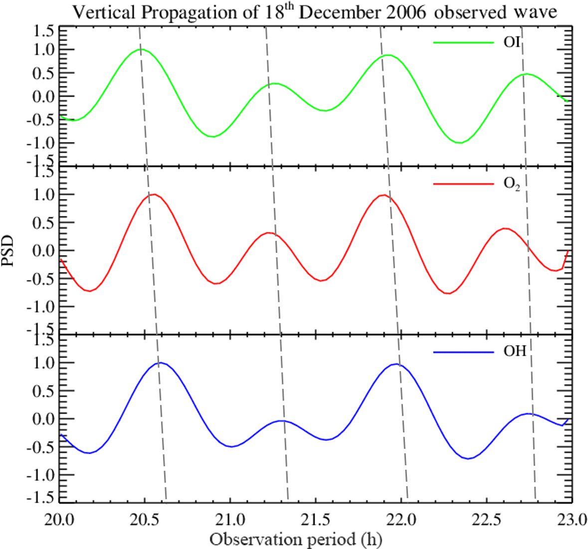
Figure 6 Downward phase propagation of the two harmonics of the 18 December 2006 observed wave.

Figure 7 Keogram of 14 October 2006.

Figure 8 Keogram 18 December 2006.

Figure 9 Results from keogram analysis for 14 October 2006.

Figure 10 Results from keogram analysis for 18 December 2006.

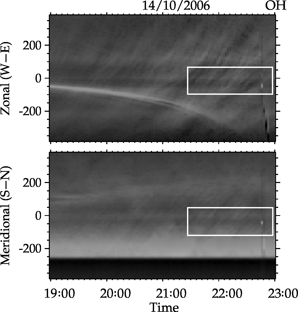
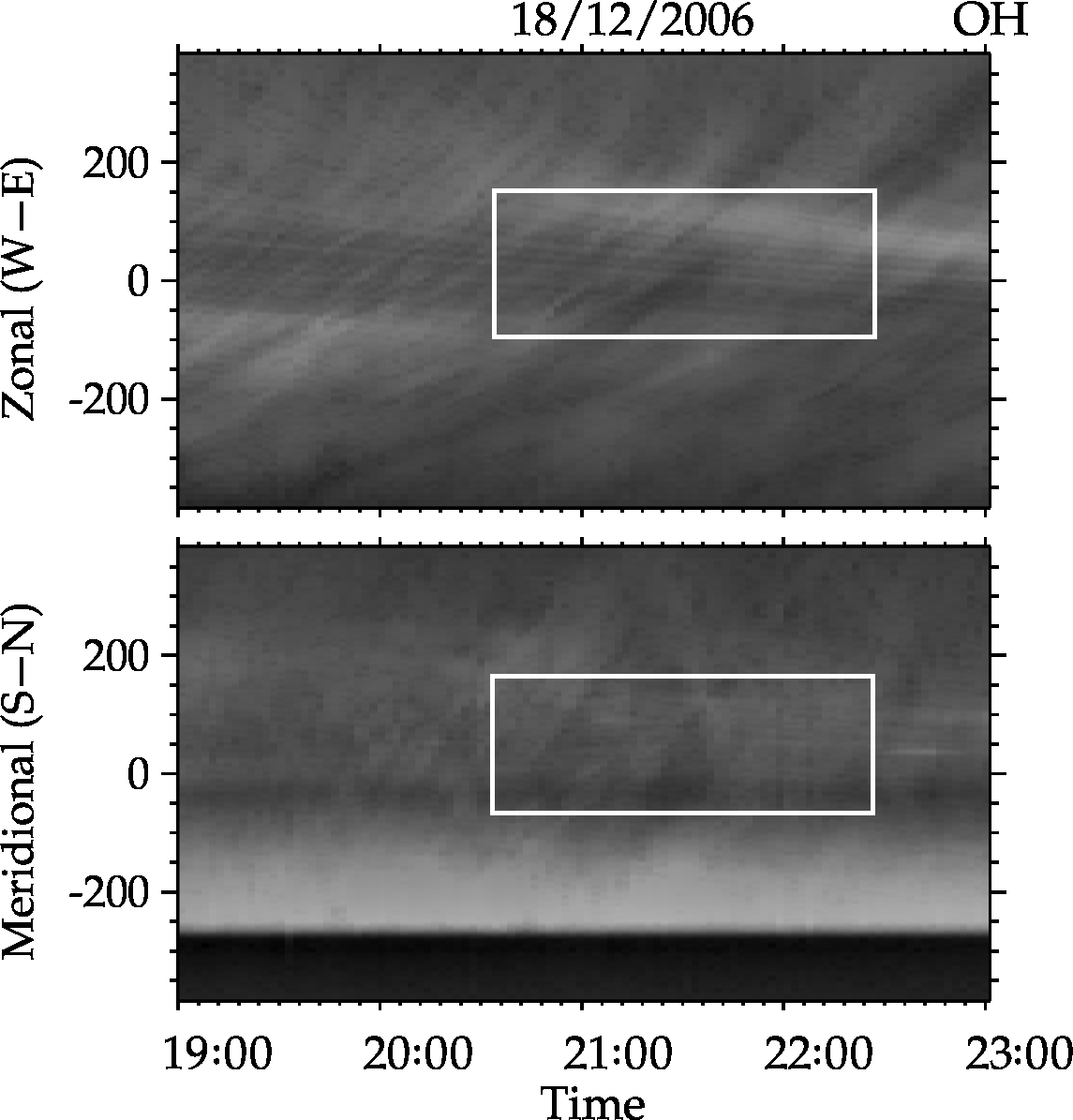
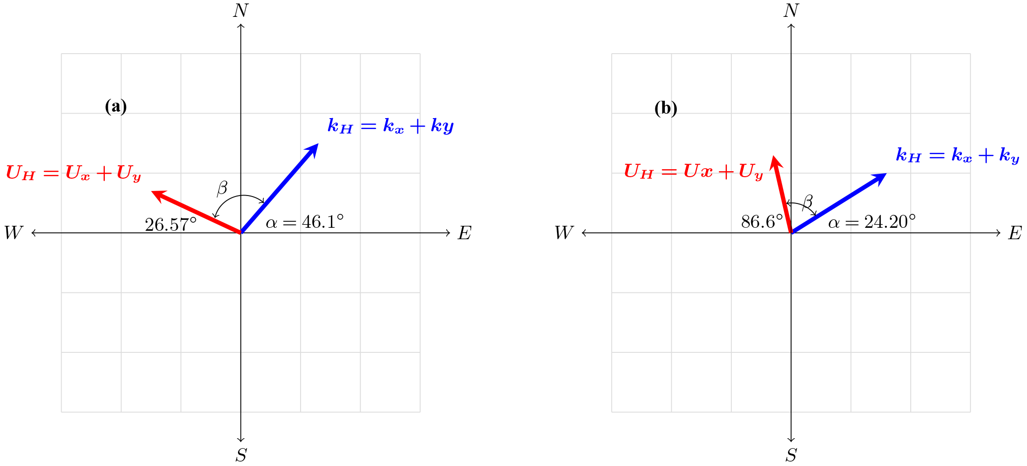
Figure 11 Vector diagram of the wave with respect to the background wind for (a) 14 October 2006 and (b) 18 December 2006 observation.

The amplitude (Rayleigh), phase (hour) and observed period (hour) obtained from the least-square fitting approach and Lomb–Scargle are shown in Table 2 for 14 October and 18 December 2006 observation, respectively.

3.2 Vertical propagation

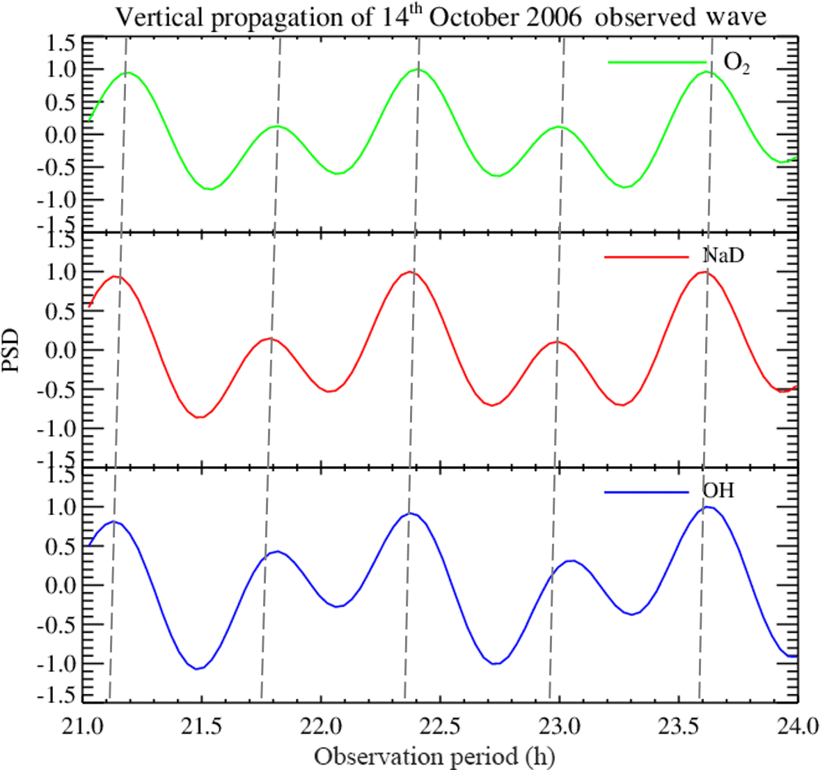
From Table 2, we observed on the night of 14 October that O₂ lags NaD by ∼ 0.10 ± 0.00 h (6.20 ± 0.00 min) with a vertical phase velocity (V_z) of $\mathrm{38.71}\pm ,\mathrm{1.16}$ km h⁻¹ (10.75 ± 0.32 m s⁻¹) and vertical wavelength (λ_z) of 23.22 ± 0.67 km, whilst NaD also lags behind OH by ± 0.05 ± 0.00 h (3.05 ± 0.09 min) with a vertical phase velocity (V_z) of 59.04 ± 1.77 km h⁻¹ (16.40 ± 0.49 m s⁻¹) and vertical wavelength (λ_z) of 35.42 ± 1.06 km. Considering the three emission layers, O₂ lags behind OH by 0.15 ± 0.01 h (9.25 ± 0.46 min) with a vertical phase velocity (V_z) of 45.41 ± 1.36 km h⁻¹ (12.60 ± 0.38 m s⁻¹) and vertical wavelength (λ_z) of 27.24 ± 0.82 km. Based on the wave parameters obtained we plot the harmonic analysis of 14 October, which is shown in Fig. 5. From Fig. 5, one can see that there is a tendency of phase delay from OH to O₂, indicating an upward phase propagation. According to the gravity wave propagation theory, upward phase propagation means downward energy propagation (Nappo, 2013).

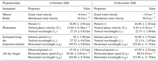
Table 3 Summary of the 14 October and 18 December 2006 observed gravity wave parameters.

Considering only two emission layers, i.e. O₂ and NaD, and NaD and OH, we found the average of their sum for the phase velocities and vertical wavelengths to be 48.88 ± 1.47 km h⁻¹ (13.57 ± 0.41 m s⁻¹) and 31.33 ± 0.94 km respectively. Comparing these with the values obtained from the direct three emission layer estimation, it is noted that there is a slight difference between the computed values. These differences can be attributed to the difference in the assumed emission altitudes of the two layers and the background wind at that layer. Statistically, the linear fitting of the altitude of the three emission layers against their respective phase has a coefficient of determination of 0.96.

Referring to Table 2 for 18 December 2006, it was revealed that, OI leads O₂ by $\sim \mathrm{0.11}\pm \mathrm{0.01}$ h (6.82 ± 0.34 min) with a vertical phase velocity (V_z) of 26.40 ± 0.79 km h⁻¹ (7.31 ± 0.22 m s⁻¹) and vertical wavelength (λ_z) of 19.36 ± 0.77 km while O₂ leads OH by ∼ 0.21 ± 0.01 h (4.27 ± 0.21 min) with vertical phase velocity (V_z) of 32.78 ± 1.31 km h⁻¹ (9.10 ± 0.36 m s⁻¹) and vertical wavelength (λ_z) of 23.93 ± 1.00 km. Considering the three emission layers; OI leads OH by $\sim \mathrm{0.33}\pm \mathrm{0.02}$ h (19.63 ± 0.98 min) with a vertical phase velocity (V_z) of 30.56 ± 1.38 km h⁻¹ (8.49 ± 0.38 m s⁻¹) and vertical wavelength (λ_z) of 23.21 ± 1.05 km. This shows that, the wave is having an upward energy propagation (a downward phase propagation). Thus, taking the average of the two emission layers, OI versus O₂, and O₂ versus OH, we found that the phase velocity and vertical wavelength were 29.59 ± 1.33 km h⁻¹ (8.22 ± 0.37 m s⁻¹) and 21.64 ± 0.97 km respectively. Comparing these with the values obtained from the three emission layers direct estimation, slight variations between the values were noted. These variations can be due to the assumed altitudes between the emission layers and the background wind at that layer. Statistically, the linear fit of the three emission layers (altitude against their corresponding phase) have a coefficient of determination of 0.97. Figure 6 shows the downward phase propagation of the 18 December 2006 observed wave.

3.3 Keogram analysis

Figures 7 and 8 are the OH NIR co-located keogram developed from the unwarped images obtained from the all-sky imager of the same waves observed in the photometer data on 14 October and 18 December 2006. The results of the spectral analysis obtained are shown in Figs. 9 and 10.

For the case of 14 October 2006 (Fig. 9), the period of the horizontal component of the wave is 0.55 ± 0.03 h (33.30 ± 1.70 min) propagating at 334.80 ± 16.74 km h⁻¹ (93.00 ± 7.30 m s⁻¹) and having a horizontal wavelength of 185.80 ± 10.09 km with an azimuthal angle of 64^∘ suggesting that, the horizontal component of the wave is northeastward.

Similarly, Fig. 10 shows the result from the all-sky image of 18 December 2006. The intrinsic period of the horizontal component of the wave is 0.73 ± 0.04 h (43.90 ± 2.20 min) propagating at 88.90 ± 6.90 m s⁻¹ with a horizontal wavelength of 233.90 ± 14.00 km moving at 65.8^∘ from the azimuth and showing that the wave on this day is propagating northeastward. To estimate the influence of the background wind, coincident meridional and zonal wind velocities were taken from the Meteor radar.

The coincident measurement of the horizontal component of the wave using the all-sky imager and the background wind velocity from the Meteor radar jointly gave the general insight about the interaction of the wave with the background wind. The background wind velocity was smoothed by a 3 h running average. Using the zonal and meridional wind velocities, the magnitude and the direction of the winds were also estimated. With these two parameters, the angle (β) that the wind made with the wave was found to be 89.6^∘, indicating that the wind was moving northwestward. By using the projection method of the dot product (Dray and Manogue, 2006), the intrinsic frequency obtained using Eq. (6) was found to be $\mathrm{2.74}\times {\mathrm{10}}^{-\mathrm{3}}$ s⁻¹ (38.19 min) and the observed frequency to be $\mathrm{2.91}\times {\mathrm{10}}^{-\mathrm{3}}$ s⁻¹ (33.30 min) for the case of 14 October 2006. This value was confirmed using the inner product method, where the angle ($\mathit{\alpha }=\mathrm{46.1}{}^{\circ }$), their respective wind velocity and wave numbers were used in this estimation. The inner product method also yielded the same result for the intrinsic frequency. From the dispersion relation for gravity waves (Eq. 4), the estimated value for the horizontal wavelength (λ_H) is 195.93 ± 9.80 km.

For 18 December 2006, the angle (β) that the wind made with the wave was found to be 69.2^∘. By using the projection method of the dot product, the intrinsic frequency was found to be $\mathrm{1.91}\times {\mathrm{10}}^{-\mathrm{3}}$ s⁻¹ (54.00 min), whereas the observed frequency was $\mathrm{2.39}\times {\mathrm{10}}^{-\mathrm{3}}$ s⁻¹ (43.90 min). Applying the same inner product approach used earlier, we found that the angle (α) the wave made with the azimuth was 24.2^∘. This agreed with the estimated value obtained using the projection method. Their respective wind and wave numbers were used in this estimation. The inner product method also yielded the same result for the intrinsic frequency. From the dispersion relation for gravity waves, the estimated value for the horizontal wavelength is 235.66 ± 11.78 km. The estimated values from our analysis for the two cases are shown in Table 3.

4 Conclusions

The simultaneous observation of similar gravity wave periods within the three airglow emission layers in the photometer data suggests a vertical propagation of the same gravity wave. The observed waves propagated through the emission altitudes OH (87 km), NaD (90 km) to O₂ (94 km) for the case of 14 October 2006, whereas that of 18 December 2006 propagated through OH (87 km), O₂ (94 km) to OI (97 km). From our observation, the amplitude growth reflects theory and agrees reasonably with previous observational works done (e.g. Taori et al., 2007; Taori and Kamalakar, 2013; Takahashi et al., 2011; Ghodpage et al., 2014).

Using the wind data from the meteor radar, the intrinsic frequency of the vertical (either upward or downward) phase propagation was estimated using Eq. (6). With the estimated intrinsic frequency, the horizontal wavelength was estimated using the dispersion relation of gravity waves (Vadas and Liu, 2009) and compared to the horizontal wavelength obtained from the keogram analysis of the simultaneously observed OH images. Both the analytical and numerical results of the horizontal wavelength agree reasonably, hence suggesting that the same wave was observed by the photometer and the all-sky imager. The observations of the same wave in both instruments allow the investigation of the two-dimensional properties of the waves.

From the case study on the night of 14 October and 18 December 2006, we observed two different wave propagation modes, one had an upward phase propagation while the other had a downward phase propagation. The latter is well known as upward propagation of gravity wave (Fritts and Alexander, 2003). However, the former can not be explained by the upward propagating gravity waves. In order to further investigate the present case we have to know more about the background atmosphere (wind and temperature, for example).