Mesopause region temperature variability and its trend in southern Brazil

Nowadays, the study of the upper atmosphere is increasing, mostly because of the need to understand the patterns of Earth's atmosphere. Since studies on global warming have become very important for the development of new technologies, understanding all regions of the atmosphere becomes an unavoidable task. In this paper, we aim to analyze the temperature variability and its trend in the mesosphere and lower thermosphere (MLT) region during a period of 12 years (from 2003 to 2014). For this purpose, three different heights, i.e., 85, 90 and 95 km, were focused on in order to investigate the upper atmosphere, and a geographic region different to other studies was chosen, in the southern region of Brazil, centered in the city of Santa Maria, RS (29^∘41^′02^′′ S; 53^∘48^′25^′′ W). In order to reach the objectives of this work, temperature data from the SABER instrument (Sounding of the Atmosphere using Broadband Emission Radiometry), aboard NASA's Thermosphere Ionosphere Mesosphere Energetics Dynamics (TIMED) satellite, were used. Finally, two cases were studied related to distinct grids of latitude/longitude used to obtain the mean temperature profiles. The first case considered a grid of 20^∘ × 20^∘ lat/long, centered in Santa Maria, RS, Brazil. In the second case, the region was reduced to a size of 15^∘ × 15^∘ in order to compare the results and discuss the two cases in terms of differences or similarities in temperature trends. Observations show that the size of the geographical area used for the average temperature profiles can influence the results of variability and trend of the temperature. In addition, reducing the time duration of analyses from 24 to 12 h a day also influences the trend significantly. For the smaller geographical region (15^∘ × 15^∘) and the 12 h daily time window (09:00–21:00 UT) it was found that the main contributions for the temperature variability at the three heights were the annual and semi-annual cycles and the solar flux influence. A smaller trend (−0.02 ± 0.16 % decade⁻¹) was found at 90 km height and small positive trends (0.58 ± 0.26 % and 0.41 ± 0.19 % decade⁻¹) were found at altitudes of 85 and 95 km, respectively..

Keywords. Atmospheric composition and structure (middle atmosphere – composition and chemistry; pressure, density, and temperature) – meteorology and atmospheric dynamics (climatology)

1 Introduction

The upper atmospheric region (mesosphere and lower thermosphere – MLT) is gradually becoming more important due to the climate change debate. The magnitude of impact predicted for the MLT region is expected to occur sooner and higher than at tropospheric heights (Beig, 2002). In this way, temperature measurements in the lower and middle atmosphere have been conducted for several decades by different authors (e.g., Aikin et al., 1991; Batista et al., 2008; Berger et al., 2011; Lübken et al., 2013) for a variety of scientific studies, including meteorological and climatological purposes. On the other hand, the upper atmosphere (above ∼ 90 km) has not been focused on in the majority of past research due to the difficulty in measuring at these heights.

One of the many instruments used to investigate the upper atmospheric region is the SABER (Sound of the Atmosphere using Broadband Emission Radiometry) on board the TIMED (Thermosphere, Ionosphere Mesosphere, Energetics Dynamics) satellite. Several reports of comparisons between SABER temperatures and those measured by ground-based techniques have been published in recent years (e.g., Mertens et al., 2004; Oberheide et al., 2006; Mulligan and Lowe, 2008; Remsberg et al., 2008; Smith et al., 2010). All of these studies involve relatively short data runs and focused on intercomparisons of several data from Northern Hemisphere regions. The work of French and Mulligan (2010) differed from previous studies in the following respects: it used ground-based temperature data from a Southern Hemisphere station – Davis Station, Antarctica (68^∘ S, 78^∘ E) – and it included the years 2002–2009, which enabled the behavior of the bias between SABER and the Davis dataset during this extended period to be examined.

Many investigations related to temperature trends have been conducted in different geographic regions and at a range of altitudes and have estimated several temperature trends. Several different techniques have been used around the globe to analyze temperature trends in the middle and upper atmosphere. Semenov and Shefov (1999) and Reisin and Scheer (2002) used hydroxyl rotational temperature techniques and estimated trends lower than −7 K decade⁻¹. Semenov and Shefov (1999) analyzed 44 years of UARS satellite data in a grid of 14^∘ × 6^∘ lat/long centered at 49^∘ N, 40^∘ E. Resin and Scheer (2002) considered separate years (from 1986 to 2001) in the region of 31.8^∘ S, 69.2^∘ W. Offermann et al. (2003) and Lowe (1999, 2002) used the same technique as used previously; however, both found slightly positive temperature trends. The works were conducted over 19 years in the region of 51.3^∘ N, 7^∘ E and for 13 years located in the region of 43^∘ N, 81^∘ W, respectively. The previous works mentioned focused on the heights of 80–95 km. Reisin and Scheer (2002) studied the years of 1968–2000 using O₂ rotational temperature analysis at a height of 95 km. Focusing on the region of 31.8^∘ S, 69.2^∘ W, a temperature trend of −0.3 (±1.5) K decade⁻¹ was calculated. Huang et al. (2014) estimated that the temperature trend in the upper mesosphere (between 85 and 100 km) could approach, approximately, −3 K decade⁻¹. As the amplitude of temperature variation increases with respect to altitude due to the decrease in density, the effects of climate change are likely to be more pronounced at higher altitudes (Kishore, 2014).

As noted, most studies were conducted in regions of middle and high latitude. Thus, the study of low-latitude regions is not widely explored. Several authors have studied the temperature in the middle and upper atmosphere over the Brazilian territory, utilizing different methods and techniques for temperature measurements, but not using specific models for trend and variability analyses as in our investigation described here. Among the previous utilized techniques are the airglow OH emission measurements (Takahashi et al., 1995), vertical distribution of atmospheric sodium (Clemesha et al., 2004), OH rotational temperature measurements (Clemesha et al., 2005) and Rayleigh lidar (Batista et al., 2009), but these studies were not focused on the upper mesosphere–lower thermosphere over the southern region of Brazil, which is a region with very well defined seasons and which is very interesting for these studies.

In this paper temperature data from TIMED/SABER instrument in the region of 80–100 km altitude from the years 2003 to 2014 were used to inspect the temperature variability and temperature trend over southern Brazil and surrounding areas. The focus was on three different heights, i.e., 85, 90 and 95 km, in order to investigate the MLT region. In addition to that, the influences of solar cycles and natural cycles in the monthly temperature variability around the mesopause were verified.

2 Instrumentation and data

In this study, data from the TIMED/SABER satellite were used for the assessment in the upper mesosphere. The Trend-Run model was used to study the temperature trends in this region in the atmosphere (Toihir et al., 2014).

It is know that the mesopause may vary its position through the years. In addition, the studied geographical area can influence the height of mesopause once it changes around the globe.

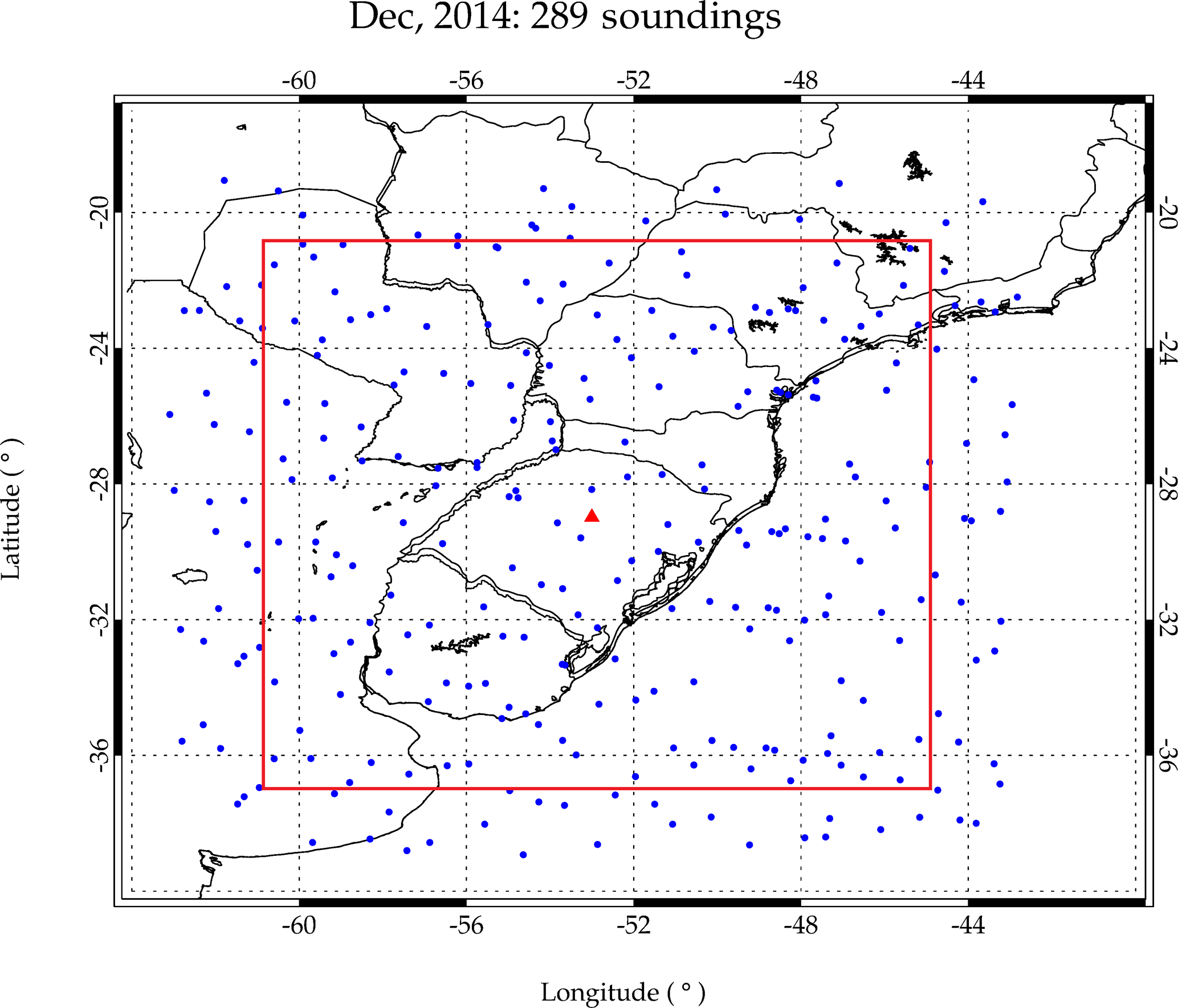
Figure 1 Example of SABER/TIMED sounding locations (blue dots) during December 2014, over the Santa Maria location (red triangle) within a grid of ±10^∘ in latitude and longitude (lat/long). The red box corresponds to the main and smaller region delimited within ±7.5^∘ lat/long.

The geographical area chosen for the present study was the southern Brazil region, Uruguay and portions of Argentina and Paraguay, centered at Santa Maria (29^∘41^′ S, 53^∘48^′ W), denoted by a red triangle in Fig. 1. The temperature data were obtained for two latitude and longitude configured grids. The first grid was 20^∘ × 20^∘ lat/long, and for the second case, a 15^∘ × 15^∘ grid was chosen. In both cases, the altitude range for which the SABER individual profiles were taken was from 80 to 100 km. The TIMED/SABER satellite soundings, from which the daily average temperature profiles were obtained, are in blue.

It can be seen from Fig. 1 that the soundings used for the first case cover a vast region. So, it can be difficult to understand how the temperature has varied over time in that region, since it covers sites with very different temperatures; consequently there is large variance in the daily mean temperatures.

Reducing the observed area from 20^∘ × 20^∘ to 15^∘ × 15^∘, it is found that the amount of data available for analysis was reduced to around 75 % of the total data. However, less variance in the monthly averages was observed and, consequently, there were smaller standard deviations in the mean monthly temperature.

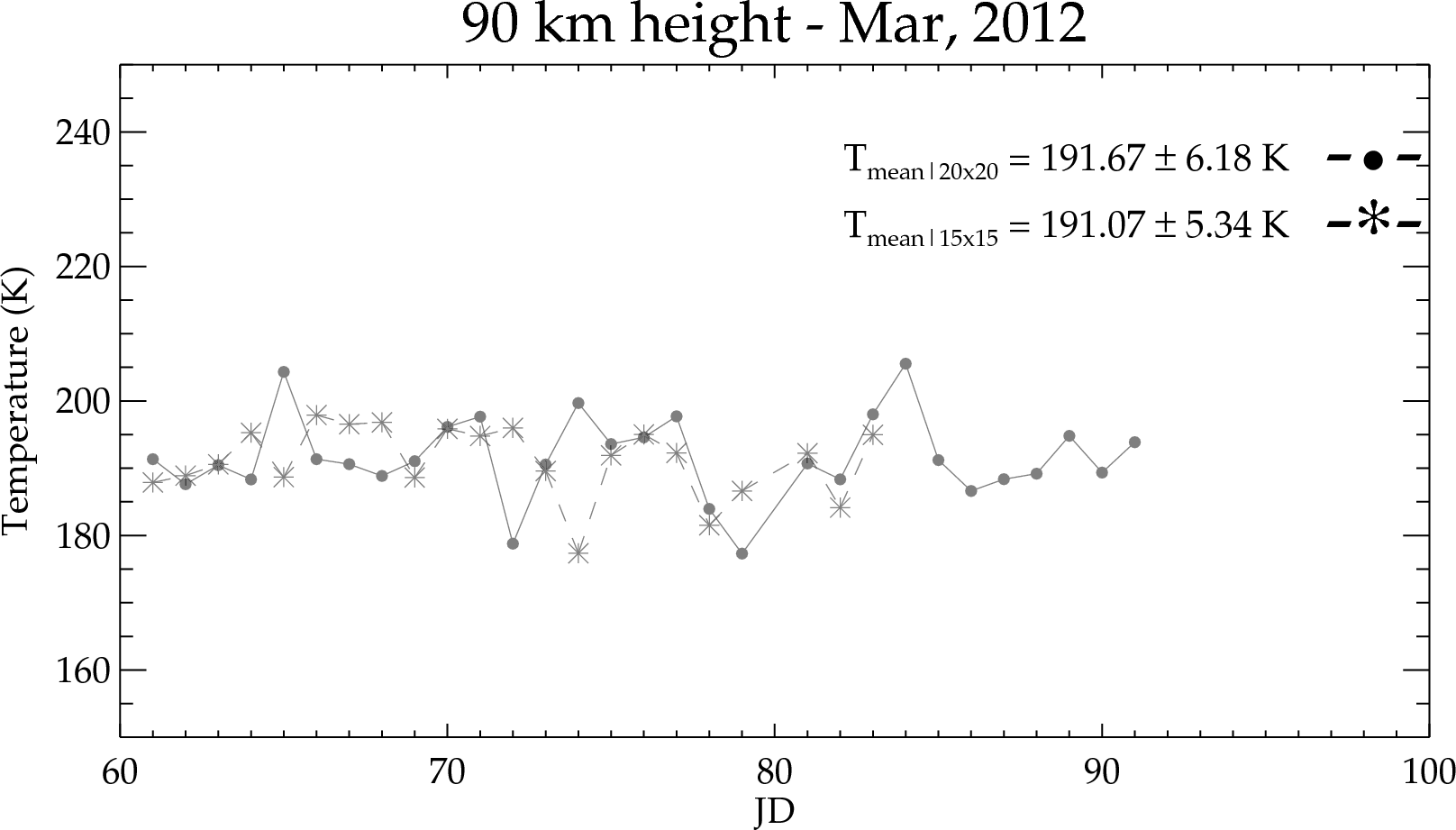
Figure 2 Daily mean temperature evolution at 90 km height as derived from SABER/TIMED profiles during March 2012 comparing both 20^∘ × 20^∘ (•) and 15^∘ × 15^∘ (∗) lat/long grids.

The time series of daily average temperature for March 2012 in the 20^∘ × 20^∘ and 15^∘ × 15^∘ grids is shown in Fig. 2, which is later used to obtain the mean temperature for this month. The same process is applied to all the months for the period from 2003 to 2014 in order to obtain a complete series of monthly temperatures, which, in turn, will be analyzed for its variability and trends. This analysis was applied for both 20^∘ × 20^∘ and 15^∘ × 15^∘ cases at the heights mentioned before.

It is possible to observe in Fig. 2 that there are peaks of maximum and minimum temperature in the time series and different agents, such as planetary waves or other oscillations in the MLT region, which could explain the possible cause of such peaks. In addition, it is noted in the 15^∘ × 15^∘ grid that there are three minimums on days 74, 78 and 82, which can be associated with a 4-day planetary wave, but larger oscillations can also modulate the temperature, and the breaking of gravity waves can contribute to the temperature variability at this height.

In order to compare the 20^∘ × 20^∘ and 15^∘ × 15^∘ grids, the time series of daily temperature averages for 24 h a day was analyzed for March 2012. The results of this comparison are shown in Fig. 2. It is possible to observe that there are oscillations with distinct periods, depending on the grid used; that is, in the 15^∘ × 15^∘ grid, a 4-day period is evident and in the 20^∘ × 20^∘ grid, a 7-day period is evident (minimums on days 72, 79 and 86), associated with planetary waves' motion. Each different grid presents distinct mean temperature values; that is, in the 15 × 15^∘ grid the mean temperature and standard deviations are smaller than in the 20^∘ × 20^∘ grid. Another way to reduce the variance in the temperature means is to limit daily analysis from 24 to 12 h, once that SABER passages occur about twice a day (Reisin and Scheer, 2017). In this paper, considering this limitation of time and also to avoid the contamination of daily oscillations with 12 or more hours of periods (thermal tides), a period from 09:00 to 21:00 UTC was chosen to obtain the daily mean temperature profiles.

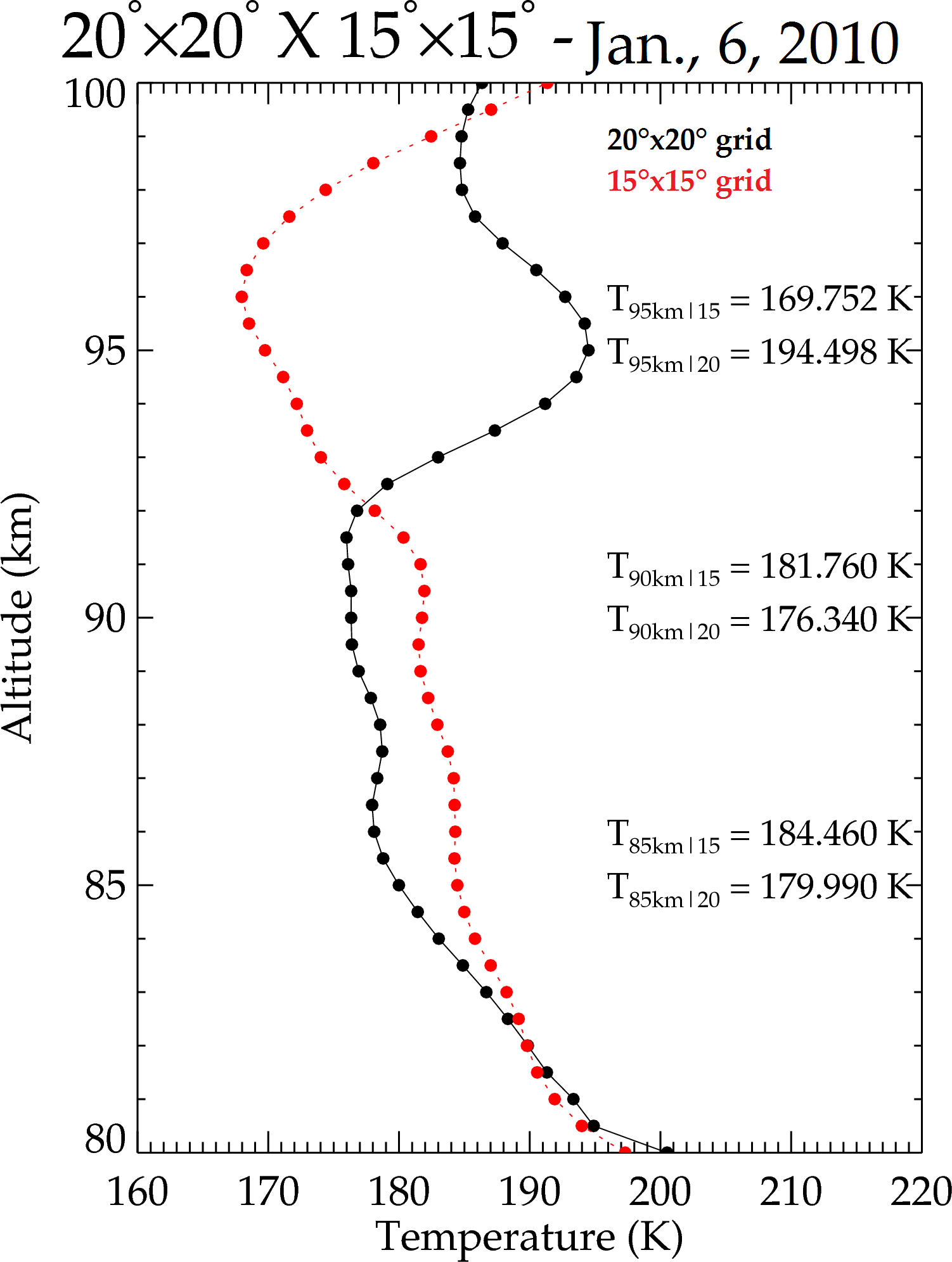
Figure 3 Temperature profiles of the MLT region as retrieved from SABER/TIMED observations over Santa Maria, southern Brazil, on 6 January 2010. The 20^∘ × 20^∘ lat/long grid profile is shown in black, while the 15^∘ × 15^∘ profile is shown in red.

One example of a daily mean temperature profile for 6 January 2010 for the 20^∘ × 20^∘ grid compared with the 15^∘ × 15^∘ grid in 24 h of data is shown in Fig. 3. In this figure, it can be noticed that the lowest temperature of the day is located at about 91.5 km height, with a value of ∼ 176.5 K, for the 20^∘ × 20^∘ grid. For the 15^∘ × 15^∘ grid it can be seen that the lowest temperature is located at about 96 km height, with a value of 167.85 K. The second case appears to be closer to the behavior of the MLT region, a decrease of the temperature until the mesopause (height of lowest temperature) and then an increase throughout the thermosphere. Thus, further analyses are conducted in this case.

In order to show that limiting the time of analysis influences the daily temperature profile, Fig. 4 presents a comparison between 24 and 12 h analysis using the 15^∘ × 15^∘ grid. It is possible to see that a 12 h analysis presents a behavior even closer to that expected for the MLT region. The lowest temperature is located at about 96 km height, with a value of ∼ 163.8 K. Thus, an analysis of 12 h in the 15^∘ × 15^∘ grid is expected to have better results of temperature trend and variability in the upper atmosphere. Consequently, further analyses are conducted considering only the 15^∘ × 15^∘ grid and only for the daylight period (12 h a day).

2.1 TIMED/SABER satellite

The TIMED satellite was launched in December 2001 aboard the Delta II launch vehicle at Vanderberg Air Force Base, California. The TIMED satellite helps supply data for studies of the influences of the Sun and human activity in the MLT region. This region is the passage between space and the terrestrial environment, where solar energy is first deposited (Russell et al., 1999).

The experiments onboard TIMED are focused on a portion of the atmosphere located at about 60–180 km height. The TIMED payload consists of a set of four instruments, one of which is the SABER instrument used in this work. The SABER instrument is an infrared radiometer designed to measure the heat emitted by the atmosphere over a wide range of altitude and spectra.

The main objectives of the SABER instrument are to explore the MLT region to determine the energy balance, the atmospheric structure (such as temperature, density and pressure) and atmospheric variation according to the altitude, geographical locations and time (Huang et al., 2010). Errors in the retrieved temperatures in the 80–100 km region are estimated to be in the range from ±1.5 to 5 K if the kinetic temperature profile does not have a pronounced vertical structure (García-Comas et al., 2008). Different from other satellites, TIMED acts in such a way that SABER collects data 24 h a day, allowing the identification of diurnal variation of ozone concentration and temperature (e.g., thermal tides). This is important in the MLT region since the diurnal variation of ozone and temperature may be dominant (Huang et al, 2014).

The data obtained by SABER provided individual daily temperature profiles unequally spaced in altitude. In order to solve this problem the data were linear interpolated at each 0.5 km in altitude from 80 to 100 km and then the daily averaged temperature profiles were obtained.

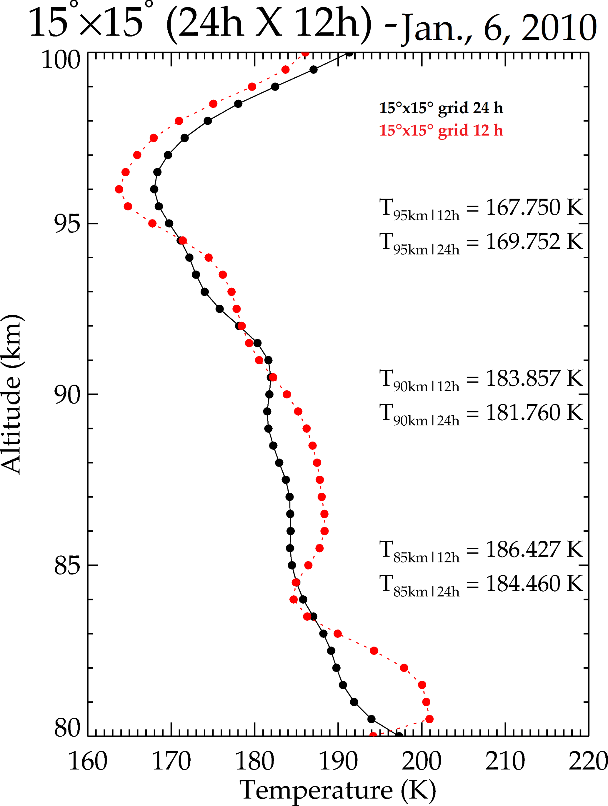
Figure 4 Temperature profiles of the MLT region as retrieved from SABER/TIMED observations over Santa Maria, southern Brazil, on 6 January 2010, but comparing a 24 and a 12 h analysis in the 15^∘ × 15^∘ grid. The 24 h analysis is shown in black; note that this is the same profile shown in Fig. 3. In red, the 12 h analysis is shown.

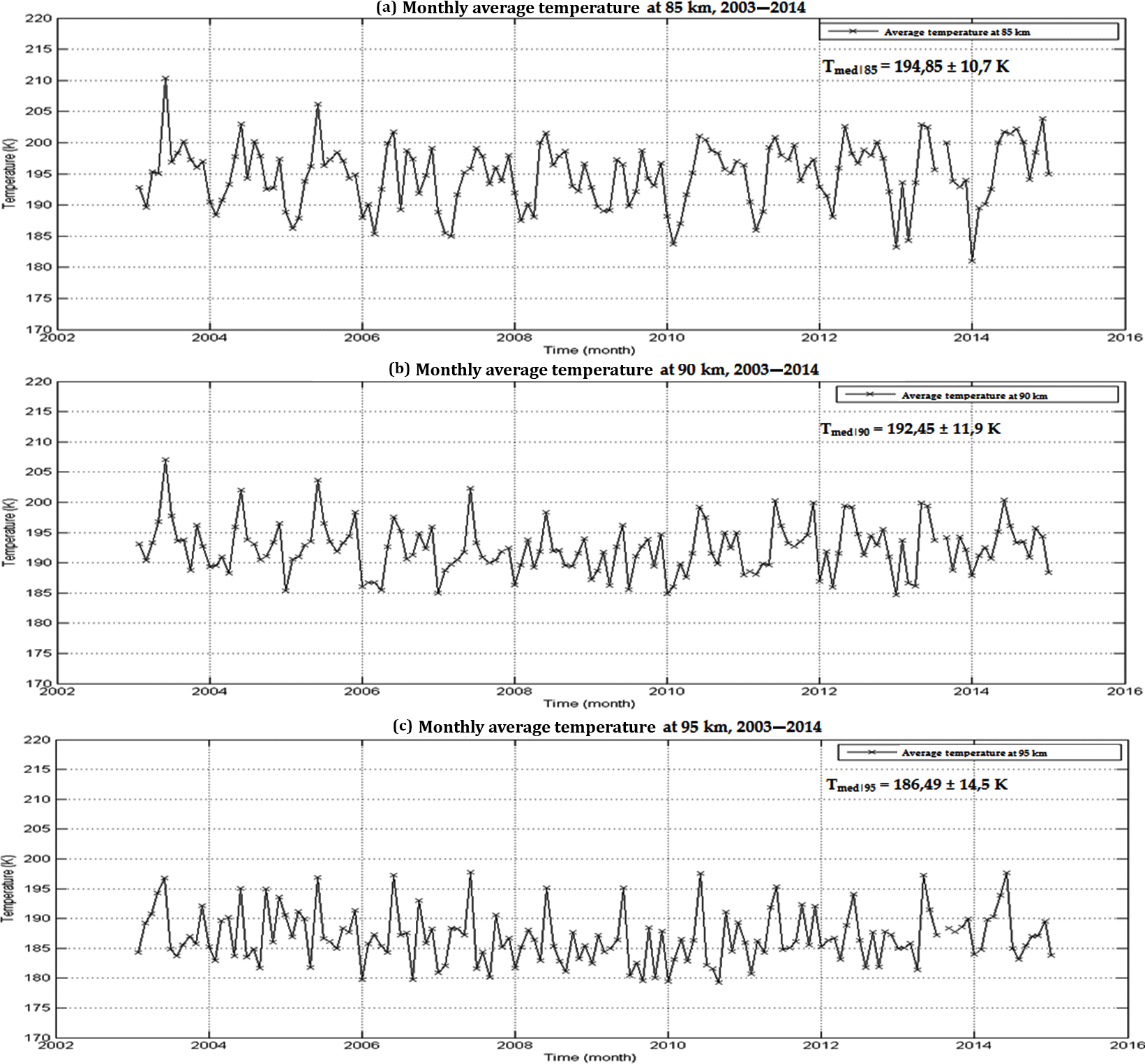
Figure 5 Monthly average temperature values at 85 (a), 90 (b) and 95 (c) km height derived within a ±7.5^∘ grid over Santa Maria, for the 2003–2014 period.

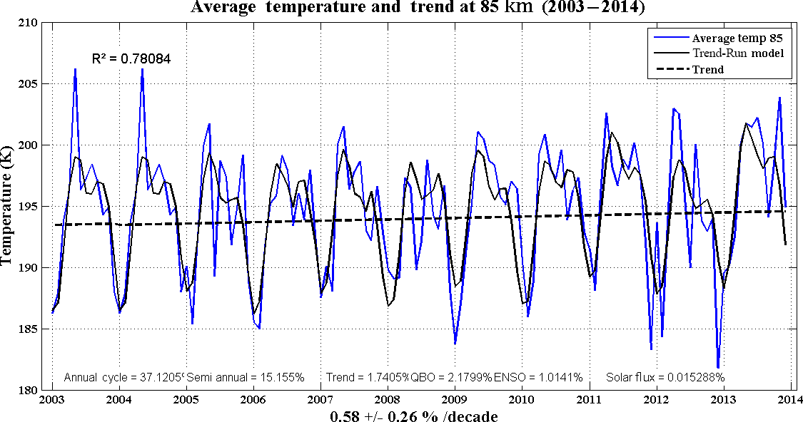
Figure 6 Time evolution of monthly averaged temperature values at 85 km height over Santa Maria, within a ±7.5^∘ grid. The dashed straight line indicates the obtained linear trend (+0.58 ± −0.26 % K decade⁻¹) from the Trend-Run model.

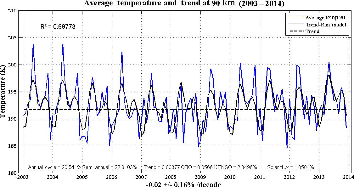
Figure 7 Time evolution of monthly averaged temperature values at 90 km height over Santa Maria, within a ±7.5^∘ grid. The obtained linear trend is −0.02 ± −0.16 % K decade⁻¹.

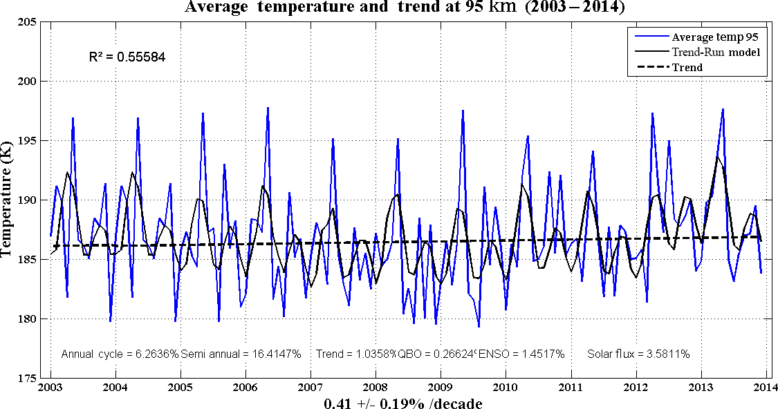
Figure 8 Time evolution of monthly averaged temperature values at 95 km height over Santa Maria, within a ±7.5^∘ grid. The obtained linear trend is +0.41 ± −0.19 % K decade⁻¹).

2.2 Trend-Run model

One of the methods applied for temperature trend analysis is based on a linear regression model that is called Trend-Run, which is adapted from AMOUNTS (Adaptive Model Unambiguous Trend Survey) and AMOUNTS-O3 models, specially developed for ozone and temperature trend analysis (Hauchecorne et al., 1991; Keckhut et al., 1995; Guirlet et al., 2000).

Trend-Run is, therefore, a statistical model that has been adapted and used to estimate the trend of temperature over the years whose data were used (Bencherif et al., 2006). The model is based on the principle of breaking the series of time variation Y(t) into sums of different parameters that explain the Y(t) variation:

$$\begin{array}{ll}{\displaystyle }& {\displaystyle }Y(z,t)=c_{\mathrm{1}}\mathrm{SAC}(z,t)+c_{\mathrm{2}}\mathrm{AC}(z,t)+c_{\mathrm{3}}\left(z\right)\mathrm{QBO}(z\mathrm{40},t)\\ \text{(1)}& {\displaystyle }& {\displaystyle }+c_{\mathrm{4}}\left(z\right)\mathrm{ENSO}\left(t\right)+c_{\mathrm{5}}\left(z\right)\mathrm{SSN}\left(t\right)+\mathit{\epsilon }(z,t).\end{array}$$

The Trend-Run model (represented by Eq. 1) considers the main parameters such as annual (AC) and semi-annual cycles (SAC), QBO (quasi-biennial oscillation), ENSO (El Niño–Southern Oscillation), and the 11-year cycle (Sunspot Number), in addition to a residual term ε, assuming a consistent trend (Bègue et al, 2010). In this way, the contribution that each of these cycles or oscillations makes to the temperature variance may be estimated.

When the coefficients c_i (i=1, …, 5) are calculated, the corresponding parameters are removed from the studied geophysical signal Y(t). Applying the ordinary least-squares method, the model minimizes the sum of quadratic residuals and thus determines the coefficients of parameter c_i. In relation to the trend, there is a linear parameterization, defined by

$$\begin{array}{}\text{(2)}& \mathrm{Trend}\left(t\right)={\mathit{\alpha }}_{\mathrm{0}}+{\mathit{\alpha }}_{\mathrm{1}}t.\end{array}$$

In the trend equation, t denotes the time interval, α₀ is a constant and α₁ is the slope of the straight trend (t), which estimates the trend along the timescale.

3 Results and discussion

3.1 Monthly temperature averages

As commented in Sect. 2, the following results were found using the 15^∘ × 15^∘ grid in a 12 h analysis at three different height levels (85, 90 and 95 km). After the acquisition and analysis of daily temperature data, a monthly average temperature time series was set up to facilitate the study of temperature variability. Each height was studied separately, and the results are shown in the following.

The monthly average temperature at three separate heights, between 2003 and 2014, for the 15^∘ × 15^∘ grid, centered at Santa Maria, RS, Brazil, is shown in Fig. 5. In the years 2003 and 2014 the average temperature in the upper atmosphere is higher than the other analyzed years. One cause of this is that the solar cycle (in addition to other agents) is at its peak in those years. The year of 2003 is the beginning of this cycle and 2014 is the end. It is also noted that the lowest average temperatures were in 2007/2008, when the solar cycle was at its minimum and the Sun was transmitting less energy (heat) to the Earth. This behavior can be seen at the three heights analyzed. Besides that, it is noted that the main minimum temperature peak is situated, mainly, in the month of January, while the principal maximum in the temperature occurs in the month of May. A secondary minimum is seen to occur in the month of August. In addition, another secondary maximum occurs in the month of November. Both the secondary maximum and minimum could be associated with the contribution of the semi-annual cycle.

The minimum average temperature occurs at 95 km, around 187 K, while the maximum is found to be at 85 km, around 195 K (not considering the standard deviation); this can be associated with the vertical profile shown in Fig. 4. Note that, in both 85 and 90 km height cases, it is possible to see a similar behavior in all years; in other words, it is possible to see a pattern over the years. That does not occur in the last case, at 95 km, since this can be possibly related to this portion being more influenced by atmosphere cycles and oscillations.

3.2 Temperature trend and variability analyses

By using the Trend-Run analysis model briefly described in Sect. 2.2, it can be identified how the MLT region temperature has varied in recent years. Also, it is possible to determine how its behavior should be in the future above the southern Brazil region.

The Trend-Run model is a statistical model that estimates the temperature trend by separating the different contributions that should influence the temperature variability through the several years of data. As this is a statistical model, the R² (correlation coefficient) shows how correlated the model is compared to the original series. When R² > 0.7, it can be stated that there is a strong correlation; i.e., Trend-Run is accurate enough for this analysis. Figure 6 shows the compatibility of the model with the time series of temperature at 85 km height. Figure 6 shows how each parameter acts with the variation of temperature and the distinct kinds of variability are identified. In this case the strongest influences in the temperature variability are the annual (37.12 %) and semi-annual (15.15 %) variation. In addition, it can be seen that the QBO has about 2.2 % influence on the temperature variability. Note that the solar flux has a rate of only 0.015 %; however, when analyzing Fig. 6, it is possible to notice that in the years of maximum solar activity (2003 and 2014) the temperature amplitude in the temperature series is about 10 K, while in the year of minimum solar activity (2008), the temperature amplitude is near 5 K. Thus, it is seen that the solar cycle influences the amplitudes of annual and semi-annual variation directly.

For the first case, in the upper mesosphere (at 85 km height), it was shown that the trend in recent years is that the temperature is increasing by 0.58 K decade⁻¹. Lowe (1999, 2002) and Semenov et al. (2002) worked around the same period of time as this paper and found similar results. The first indicated that the temperature trend at heights around 87 km would be 0.6 K decade⁻¹, while the second authors estimated the trend to be 0.3 K decade⁻¹ at similar heights. Both studies were carried out in the Northern Hemisphere.

The same analysis as before is shown in Fig. 7, but for the case of 90 km height. Again, considering the correlation coefficient, a strong correlation can be identified between the model and the temperature series. For this case, the strongest variation in the series is the semi-annual oscillation. It is possible to notice that the QBO no longer influences the trend (lower than 0.06 %) and that the solar influence tends to contribute with a small percentage (1.05 % of influence). Therefore, solar influence is clear in the years of maximum activity when temperature amplitudes of 10 K are seen. On the other hand, in the years of minimum solar activity temperature, amplitudes of around 5 K are evident.

Additionally, the temperature trend for this case was obtained as a very small value, −0.02 K decade⁻¹. Since the result is near to zero, it can be said that there is no significant trend at 90 km height. This result can be related to the ones of French (2002) and She and Krueger (2003). Both works found no significant trend in their studies.

The temperature trend analysis for the 95 km height case is presented in Fig. 8. This time, R²<0.7; therefore, the model does not indicate strong accuracy within the temperature measurements. However, it still can be relied on since the oscillations are well represented by the model and only the peak intensities cannot be captured accurately by the Trend-Run model. The strongest influence continues to be the semi-annual oscillation. It is possible to see that the solar influence intensifies (3.5 % in this case). Although the solar influence has increased, it is difficult to see the same pattern of solar activity throughout the years as in the other cases. It may be related to other influences in this portion of the atmosphere that were not removed due to the limitations of this trend model. The temperature trend found for this case is 0.41 K decade⁻¹. This differs from results found at this particular height which show decreasing trends, such as by Reisin and Scheer (2002) and Semenov et al. (2002).

Besides the works already mentioned, most of the upper atmosphere studies, carried out by different authors, show that the temperature trend is decreasing. In this work, no significant trend was found when comparing all three results presented here. This difference can be explained by the influence of contributions like planetary waves and their seasonality and other influences, which were not taken into account when the monthly temperature average was obtained. Even the influence of thermal tides has been removed indirectly, by analyzing only a short period of time (< 12 h) during the day, and the planetary waves were not removed from each month. But this is a task for future works that can study the climatology of planetary waves in the MLT region over southern Brazil in order to include such results in the Trend-Run model and then obtain more accurate results. Furthermore, the studied geographic region and the period of time (2003–2014) differ from previous works, which have been, in the majority of the cases, carried out in the Northern Hemisphere.

The possible influences on the temperature variability are mainly related to the semi-annual and annual cycles, the solar cycle, cycles of galactic cosmic rays and planetary waves in the upper mesosphere, among other phenomena. A complementation of SABER temperature data can be given by the AURA satellite in order to find a way to remove gaps and better organize the daily mean temperature in order to improve future works.

4 Conclusions

Using temperature data from TIMED/SABER satellite soundings, the upper mesosphere in the south of Brazil was studied in terms of temperature variability and its trend. This is important since there are few works on this subject over the Brazilian territory and none for the southern Brazil region. This work, therefore, contributed to the study of the upper atmospheric temperature behavior over southern Brazil, showing no substantial trend in the temperature in the mesosphere over the southern Brazilian region and surrounding areas, centered in Santa Maria, RS, Brazil. In this work, the results found that the temperature trend in the 15^∘ × 15^∘ case was 0.58 K decade⁻¹ at 85 km, −0.02 K decade⁻¹ at 90 km and 0.41 K decade⁻¹ at 95 km. However, since the results for temperature trends are slightly positive, it can be considered approximately zero per year and it is possible to infer that there is no variability tendency of temperature in the mesosphere. In addition, because it is a geographically poorly studied region, the lack of data also caused interference in the results of temperature trend analysis of the MLT region. However, despite the reduction in the number of days in the 15^∘ × 15^∘ grid compared to the 20^∘ × 20^∘ grid, the results and comparisons are satisfactory for the analysis of the trend in the region of study. In future works, other methods of measurement can be used as well as data from the Earth Observing System (EOS) Microwave Limb Sounder (MLS) instrument on board NASA's EOS AURA satellite, and even at other interesting sites (e.g., on sub-Antarctic islands). With the data obtained from AURA, it will be possible to fill the gaps of days without data of the SABER instrument and thus contribute to the study of the upper atmosphere climatology that has increased in recent years.