Influence of gravity waves on the climatology of high-altitude Martian carbon dioxide ice clouds

Carbon dioxide (CO₂) ice clouds have been routinely observed in the middle atmosphere of Mars. However, there are still uncertainties concerning physical mechanisms that control their altitude, geographical, and seasonal distributions. Using the Max Planck Institute Martian General Circulation Model (MPI-MGCM), incorporating a state-of-the-art whole atmosphere subgrid-scale gravity wave parameterization (Yiğit et al., 2008), we demonstrate that internal gravity waves generated by lower atmospheric weather processes have a wide-reaching impact on the Martian climate. Globally, GWs cool the upper atmosphere of Mars by ∼10 % and facilitate high-altitude CO₂ ice cloud formation. CO₂ ice cloud seasonal variations in the mesosphere and the mesopause region appreciably coincide with the spatio-temporal variations of GW effects, providing insight into the observed distribution of clouds. Our results suggest that GW propagation and dissipation constitute a necessary physical mechanism for CO₂ ice cloud formation in the Martian upper atmosphere during all seasons.

1 Introduction

Mars is the second most studied terrestrial planet due to its similarity and also differences to Earth. For example, Mars is half the size of Earth, has two very exotic dwarf satellites, Phobos and Deimos, and has an orbital tilt similar to Earth's, and it takes Mars nearly 1.9 Earth years to go around the Sun, with a much larger eccentricity than Earth (Appendix A). Thus, Mars has seasons similar to those on Earth. Studying Mars can serve, besides the aspects of habitability, as a natural fluid dynamical laboratory, where geophysicists can test the understanding and applicability of basic fluid dynamical principles. Carbon dioxide clouds have been routinely observed in the Martian atmosphere at various altitudes between ∼50 and ∼100 km (Aoki et al., 2018; Clancy and Sandor, 1998; Clancy et al., 2007; Colaprete et al., 2008; González-Galindo et al., 2011; McConnochie et al., 2010; Määttänen et al., 2010, 2013; Sefton-Nash et al., 2013; Stevens et al., 2017; Vincendon et al., 2011). It was hypothesized that these so-called high-altitude clouds are formed in the regions where temperature drops below the CO₂ condensation threshold, which were first detected in the mesosphere during Mars Pathfinder entry and descent (Schofield et al., 1997). These high-altitude clouds are to some extent analogous to the noctilucent clouds (NLCs) observed in Earth's mesosphere (Witt, 1962), which are indeed high-altitude clouds. Previous numerical simulations and observations showed that gravity-wave-induced dynamical effects such as wind fluctuations lead to the structures observed in NLCs (Jensen and Thomas, 1994; Rapp et al., 2002).

Because the mean Martian mesosphere is in general warmer than the condensation threshold, Clancy and Sandor (1998) suggested that clouds can form in pockets of cold air created occasionally by a superposition of fluctuations associated with solar tides and gravity waves (GWs). Certainly, cold temperatures are not the only physical mechanism required for CO₂ cloud formation. The microphysics calculations demonstrated the dependence of nucleation processes on the existence and sizes of condensation nuclei (Määttänen et al., 2010), and that temperature excursions of several to tens of Kelvins below the condensation threshold are required. Simulations with the Laboratoire de Météorologie Dynamique Martian general circulation model (LMD-MGCM) demonstrated that the spatial and temporal distributions of the predicted cold temperatures generally correlated with the observations of high-altitude CO₂ clouds but could not reproduce all of their features (González-Galindo et al., 2011). This study revealed the role of thermal tides in cloud formations and the authors suggested that the discrepancies could be caused by the neglect of GWs, which were neither resolved by the MGCM nor accounted for in a parameterized form (with the exception of harmonics with zero horizontal phase velocities with respect to the surface generated by the flow over topography). The role of GWs was further addressed in the work by Spiga et al. (2012), who used a mesoscale (GW-resolving) limited-area model to demonstrate for the first time with direct simulations that orographically generated waves can propagate to the mesosphere and facilitate a creation of cold air patches at supersaturated temperatures. They compared the distribution of a linear wave saturation index with observed clouds to find that the latter reasonably well coincided with regions where GWs had favorable propagation conditions.

The next step in the attempt to explain the observations of high-altitude CO₂ clouds on the globe was performed with the Max Planck Institute (MPI) MGCM coupled with a whole atmosphere GW parameterization (Yiğit et al., 2015a). It was shown that this technique can reproduce the occurrences of supersaturated temperatures in low latitudes during a vernal equinox, in good agreement with observations of mesospheric CO₂ clouds, which, however, distinctively vary with seasons (González-Galindo et al., 2011; Sefton-Nash et al., 2013), in particular, the observational study of Sefton-Nash et al. (2013) using data from NASA's Mars Climate Sounder (MCS) onboard Mars Reconnaissance Orbiter (MRO), which demonstrated that the high-altitude clouds are continuously present in the Martian atmosphere with distinct seasonal and latitudinal behavior. From a theoretical standpoint, it is thus instructive to study the seasonal behavior of CO₂ clouds in order to gain insight into the underlying processes. In this paper, we extend the approach with parameterized GWs to further assess the role of small-scale GWs in shaping spatial and seasonal variations of pockets of cold air, which are pre-requisites for CO₂ cloud formation (Listowski et al., 2014).

Propagation of GWs into the thermosphere has been studied extensively for Earth using idealized wave models (Hickey and Cole, 1988; Walterscheid et al., 2013) and general circulation models (GCMs) (Miyoshi et al., 2014; Yiğit et al., 2009). They explored the fundamental processes that control propagation and dissipation of a broad spectrum of internal waves (Yiğit and Medvedev, 2015). On Mars, numerical wave models demonstrated that GWs can propagate into the upper atmosphere and produce similar significant dynamical and thermal forcing there (Parish et al., 2009). In particular, implementation of the whole atmosphere GW scheme of Yiğit et al. (2008) into the Max Planck Institute Martian General Circulation Model (MPI-MGCM) revealed substantial dynamical effects (i.e., acceleration/deceleration) in the Martian upper mesosphere and lower thermosphere around 90–130 km, in the region of interest of this study (Medvedev et al., 2011a). Recently, upper atmospheric signatures of small-scale GW waves have routinely been observed (England et al., 2017; Yiğit et al., 2015b).

The structure of our paper is as follows: the next section describes the methods utilized in this research, describing the MPI-MGCM, the whole atmosphere GW parameterization, and the link between clouds and waves; Sect. 3 presents an analysis of the global annual mean fields; Sects. 4 and 5 analyze the seasonal variations of the mean fields, gravity wave activity, and CO₂ cloud formation. Section 6 discusses simulation results in the context of previous research and observations. A summary and conclusions are given in Sect. 7.

2 Methodology

We next describe the MGCM, outline the implemented whole atmosphere GW parameterization, how it is linked to CO₂ cloud formation in the model, and the setup of numerical experiments.

2.1 Martian General Circulation Model (MGCM)

The Max Planck Institute Martian General Circulation Model (MPI-MGCM) calculates a three-dimensional time-dependent evolution of the horizontal and vertical winds, temperature, and density of the neutral atmosphere by solving the momentum, energy, and continuity equations on a globe. The present state of the model is the result of incremental historical development. It contains the physical parameterizations of the earlier versions (Hartogh et al., 2005, 2007; Medvedev and Hartogh, 2007) and the spectral dynamical solver introduced in the work of Medvedev et al. (2011b). Of particular relevance to the subject of this paper are the parameterizations of CO₂ condensation/sublimation and the radiative heating/cooling scheme due to IR transfer by CO₂ molecules under the breakdown of the local thermodynamic equilibrium (non-LTE). The former accounts for phase transitions, sedimentation of ice particles, surface ice accumulation, and seasonal polar ice cap, thermal, and mass effects. In the latter, the atomic oxygen profile of Nair et al. (1994) and the CO₂–O quenching rate coefficient $k_{\mathit{\nu }T}=\mathrm{3.0}\times {\mathrm{10}}^{-\mathrm{12}}$ cm³ s⁻¹ were used, as described in the paper of Medvedev et al. (2015).

The simulations have been performed with the T21 horizontal spectral truncation, which corresponds to 64×32 grid-point resolution in longitude and latitude, corresponding to approximately $\mathrm{5.5}{}^{\circ }\times \mathrm{5.5}{}^{\circ }$ resolution, respectively. The current version of the model uses 67 hybrid vertical coordinates (terrain-following in the lower atmosphere gradually and changing to pressure-based in the upper atmosphere). Its domain extends into the thermosphere to 3.6×10⁶ Pa (150–160 km, depending on solar activity, temperature, etc).

2.2 Whole atmosphere gravity wave parameterization

GCMs typically have resolutions insufficient for reproducing small-scale GWs. Therefore, the influence of subgrid-scale GWs on the larger-scale atmospheric circulation has to be parameterized. The parameterizations then estimate the effects of unresolved GWs on the resolved, large-scale flow using first principles. The vast majority of GW schemes have been designed for terrestrial middle atmosphere GCMs (Fritts and Alexander, 2003) and, thus, are not well suited for dissipative media such as Earth's thermosphere and Mars' middle and upper atmosphere. We employ a GW parameterization that is specifically developed to overcome this limitation. It was described in detail in the work of Yiğit et al. (2008), and the general principles of the extension of GW parameterizations into whole atmosphere schemes have been discussed later in the work by Yiğit and Medvedev (2013). This scheme has extensively been tested for the terrestrial environment; e.g., see the works by Yiğit and Medvedev (2016) and Yiğit and Medvedev (2017) for the recent application with the Coupled Middle Atmosphere Thermosphere-2 (CMAT2) model. The parameterization was also used within the MPI-MGCM (Medvedev et al., 2015, 2016) and has recently been tested in a Venusian GCM (Brecht et al., 2018).

Physically based parameterizations usually rely on certain simplifications. In the GW scheme applied here, information about wave phases is neglected, while covariances, including the squared amplitude, are still evaluated. In particular, the scheme calculates the vertical evolution of the vertical flux of GW horizontal momentum, $\stackrel{\mathrm{‾}}{{\mathit{u}}^{\prime }{w}^{\prime }}\left(z\right)=(\stackrel{\mathrm{‾}}{u^{\prime }{w}^{\prime }},\stackrel{\mathrm{‾}}{v^{\prime }{w}^{\prime }})$, taking account of the effect of dissipation on a broad spectrum of GW harmonics. In the middle and upper atmosphere of Mars, wave damping occurs due primarily to nonlinear wave–wave interactions (breaking and/or saturation) and molecular diffusion and thermal conduction, which are accounted for through the transmissivity τ_i (Yiğit et al., 2009):

$$\begin{array}{}\text{(1)}& {\stackrel{\mathrm{‾}}{{\mathit{u}}^{\prime }{w}^{\prime }}}_i\left(z\right)={\stackrel{\mathrm{‾}}{{\mathit{u}}^{\prime }{w}^{\prime }}}_i\left(z_{\mathrm{0}}\right){\displaystyle \frac{\mathit{\rho }\left(z_{\mathrm{0}}\right)}{\mathit{\rho }\left(z\right)}}{\mathit{\tau }}_i\left(z\right).\end{array}$$

Here overbars denote an appropriate averaging, the subscript i indicates a given GW harmonic, ${\stackrel{\mathrm{‾}}{{\mathit{u}}^{\prime }{w}^{\prime }}}_i\left(z_{\mathrm{0}}\right)$ are the fluxes at a certain source level z₀, and ρ is the mass density. This formulation requires also a prescription of the characteristic horizontal scale λ_h of GWs for calculating τ_i. For the reasons described in our papers (Medvedev et al., 2011a), λ_h=300 km was adopted in the simulations. Unlike in many conventional GW schemes, no additional intermittency factors, which are often regarded as tuning factors, are used in our scheme, because the latter is included in averaging. The parameterization is called “spectral”, because it considers propagation of a broad spectrum of waves with different horizontal phase velocities c_i (or vertical wavelengths). The initial momentum fluxes of the phase speeds have a Gaussian distribution (Medvedev et al., 2011a). Note that orographically generated GWs are represented by a single harmonic c=0. The scheme takes account of interactions between GW harmonics, rather than considering them as a mere superposition of propagating waves. Therefore, it is sometimes called “nonlinear”. Finally, the parameterization is characterized as a “whole atmosphere” one to signify its physical applicability to all atmospheric layers.

The available observational constraints on GW sources in the lower atmosphere of Mars have been discussed in the work of Medvedev et al. (2011b). First, we assume horizontally uniform total momentum fluxes in the troposphere with the maximum magnitude of 0.0025 m² s⁻². Recent simulations with a high-resolution MGCM (Kuroda et al., 2015, 2016) demonstrated that the sources of small-scale waves strongly vary horizontally and with seasons and can significantly exceed this value. Thus, the current setup allows for capture of only mean GW effects and not full details. Second, there is a lack of detailed knowledge of GW spectra in the Martian atmosphere. Meanwhile, there are indications of “universality” of these spectra (Ando et al., 2012). Thus, we assume the similar spectral shape of GWs in the troposphere as on Earth. Third, we consider that the mean wind at the source level modulates the direction of propagation of GW harmonics (and their phase velocity spectrum), thus linking the GW sources to the meteorology of the lower atmosphere (Medvedev et al., 2011b; Yiğit et al., 2009). This launch level is around 260 Pa (∼8 km).

In the simulations to be presented, the vertical fluxes due to subgrid-scale GWs (Eq. 1) are computed in all grid points in a time-dependent fashion for varying atmospheric conditions. These fluxes are used for calculating GW dynamical effects, i.e., GW-induced momentum deposition (“drag”) and GW thermal effects, i.e., heating/cooling rates (Medvedev and Yiğit, 2012; Yiğit and Medvedev, 2009), which are interactively fed into the MGCM. In the absence of dissipation (τ=1), momentum fluxes per unit volume $\mathit{\rho }\stackrel{\mathrm{‾}}{{\mathit{u}}^{\prime }{w}^{\prime }}$ remain constant, and GWs do not affect the large-scale wind and temperature fields, that is, the large-scale fields that are self-consistently resolved by the MGCM. If τ falls below unity due to dissipative effects, then GWs influence the atmospheric circulation and thermal structure. This behavior represents the process in which GWs interact with the background flow continuously as they propagate upward. This implementation also alleviates the limitation of the linear breaking assumption assumed by the majority of the conventional GW parameterizations. In a realistic atmosphere GW interactions with the background atmosphere are continuous and occur in a nonlinear fashion. The rate of GW dissipation/breaking, which itself depends on the simulated flow, determines the momentum and thermal forcing.

2.3 Linking gravity waves and ice clouds

As was described above, the GW parameterization calculates covariances of wave field variables. Of particular interest is the amplitude of temperature fluctuations $\left|T^{\prime }\right|=\sqrt{\stackrel{\mathrm{‾}}{T^{\prime \mathrm{2}}}}$. Because this scheme does not provide phase information about the subgrid-scale GW field, instantaneous values of the parameterized (unresolved by the model) temperature disturbances T^′ are impossible to determine. However, $\left|T^{\prime }\right|$ quantitatively characterizes possible maxima of fluctuations in a given point, thus allowing for extension of the probabilistic approach to CO₂ cloud formation. We assume that a cloud can form if the total temperature $T-\left|T^{\prime }\right|$ drops below a certain threshold T_s. Then, we define the probability P of this event as

$$\begin{array}{}\text{(2)}& P\left(z\right)=\left\{\begin{array}{lr}\mathrm{1}& \mathrm{if}T-\left|T^{\prime }\right|\le T_{\mathrm{s}},\\ \mathrm{0}& \mathrm{otherwise}.\end{array}\right.\end{array}$$

In the paper, we loosely call it the “probability of CO₂ cloud formation”. In fact, cold temperature is a necessary but not the sufficient condition for clouds to form. The microphysics of condensation is more complex and involves an existence and characteristics of nuclei particles. Therefore, P must be treated as a certain metric introduced for quantifying conditions favoring formation of a cloud. Because of the probabilistic nature of $\left|T^{\prime }\right|$ itself, P has a meaning only after a certain averaging. For example, calculating P at every model time step within a certain time interval and dividing by the number of the step yields the probability $\mathrm{0}\le \overline{P}\le \mathrm{1}$ as a percentage of time when cloud formation was possible.

To determine T_s, we consider the Clausius–Clapeyron equation that relates pressure p and temperature T in a system consisting of two phases, as is the case for carbon dioxide (CO₂) on Mars:

$$\begin{array}{}\text{(3)}& ({\displaystyle \frac{\mathrm{d}p}{\mathrm{d}T}}{)}_{\mathrm{sv}}={\displaystyle \frac{L_{\mathrm{sv}}}{T({\mathit{\nu }}_{\mathrm{v}}-{\mathit{\nu }}_{\mathrm{s}})}},\end{array}$$

where L_sv is the latent heat of sublimation (the subscripts s and v denote the conversion from the solid to vapor phases), ν_v, and ν_s are the specific volumes for the vapor and solid phases, respectively. Since L_sv is the heat input into the system and, thus, is positive, ν_v≫ν_s, the sublimation pressure curve, is always positive and the latent heat is temperature independent. Thus, the vapor phase of carbon dioxide behaves like an ideal gas and the Clausius–Clapeyron equation can be integrated to obtain the expression for the saturation temperature T_s:

$$\begin{array}{}\text{(4)}& T_{\mathrm{s}}=\mathit{\{}{\displaystyle \frac{\mathrm{1}}{T_{\mathrm{0}}}}-{\displaystyle \frac{R\ln \left[p\right(z)/p_{\mathrm{0}}]}{L_{\mathrm{sv}}}}{\mathit{\}}}^{-\mathrm{1}},\end{array}$$

where T₀=136.3 K is the reference saturation temperature at p₀=100 Pa and $L_{\mathrm{sv}}=\mathrm{5.9}\times {\mathrm{10}}^{\mathrm{5}}$ J kg⁻¹. As suggested by previous experimental constraints (Glandorf et al., 2002) a significant degree of supersaturation is required, if microphysics of condensation is accounted for. We employ for the saturation pressure the value 1.35×p instead of p in Eq. (4). This estimate corresponds to nuclei particles with sizes bigger than 0.5 µm and was used in previous MGCM studies (Colaprete et al., 2008; Kuroda et al., 2013). The same supersaturation threshold is applied in the condensation/sublimation scheme utilized by the MPI-MGCM for explicitly accounting for resolved CO₂ phase transitions. For smaller nuclei particles, which are expected to be present in the upper atmosphere, the degree of supersaturation increases.

2.4 Martian General Circulation Model simulations

After a multi-year spinup, the model was run for a full Martian year (669 sols ∼687 Earth days) under the low-dust scenario and for low solar activity conditions. The dust scenario represents a composite of measurements by the Thermal Emission Spectrometer onboard Mars Global Surveyor (MGS-TES) and the Planetary Fourier Spectrometer onboard Mars Express (MEX-PFS) with the global dust storms removed. Two full-Martian-year experiments have been performed: without GWs included (EXP0) and with the GW scheme turned on (EXP1). The results to be presented are based on daily averaged output data.

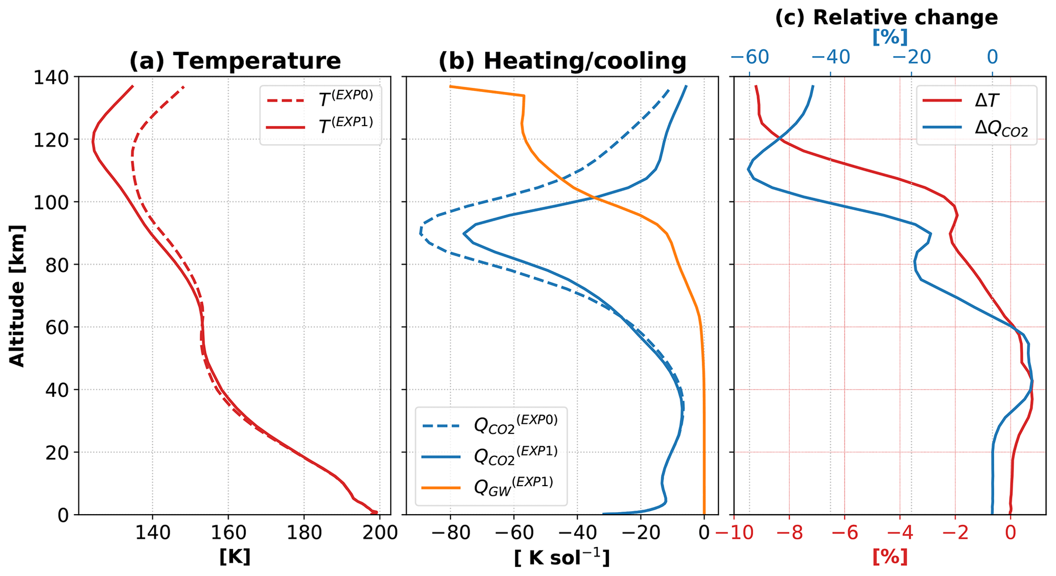
Figure 1 Global annual mean temperature, and cooling by gravity waves and radiative processes in carbon dioxide molecules. (a) Globally averaged annual mean neutral temperature (T, K) with gravity waves (solid line, “EXP1”) and without gravity waves (dashed lines, “EXP0”); (b) globally averaged annual mean gravity wave heating/cooling Q_GW (K sol⁻¹) (orange line) and CO₂ 15 µm cooling (blue line); (c) relative percentage change with respect to EXP0 simulations for the temperature (red) and CO₂ cooling (blue), calculated as $[T^{\left(\mathrm{EXP}\mathrm{1}\right)}-T^{\left(\mathrm{EXP}\mathrm{0}\right)}]/T^{\left(\mathrm{EXP}\mathrm{0}\right)}$ and $[Q_{{\mathrm{CO}}_{\mathrm{2}}}^{\left(\mathrm{EXP}\mathrm{1}\right)}-Q_{{\mathrm{CO}}_{\mathrm{2}}}^{\left(\mathrm{EXP}\mathrm{0}\right)}]/Q_{{\mathrm{CO}}_{\mathrm{2}}}^{\left(\mathrm{EXP}\mathrm{0}\right)}$. In both panels dashed lines represent the simulation without gravity wave effects, while the solid lines are for the simulation with gravity wave propagation from the lower atmosphere upward. The annual mean refers to an averaging over 1 Martian year (669 sols = 687 Earth days) over all longitudes and latitudes.

3 Mean fields, gravity waves, and probability of CO₂ ice cloud formation at solstice and equinox

Gravity waves can facilitate CO₂ cloud formation in two ways: (a) by cooling down the large-scale atmosphere globally, thus bringing its temperature closer to the condensation threshold, and (b) by locally creating pockets of cold air. In this section, we explore the former effect by comparing the EXP0 (no-GW run) and EXP1 (GW-run) simulations. It is instructive to compare the effects produced by GWs with the other major cooling mechanism in the middle and upper atmosphere of Mars – cooling due to radiative transfer in the IR CO₂ bands. A detailed study of the two mechanisms using two Martian GCMs has been performed for a vernal equinox (Medvedev et al., 2015). Here our emphasis is on the global and seasonal effects.

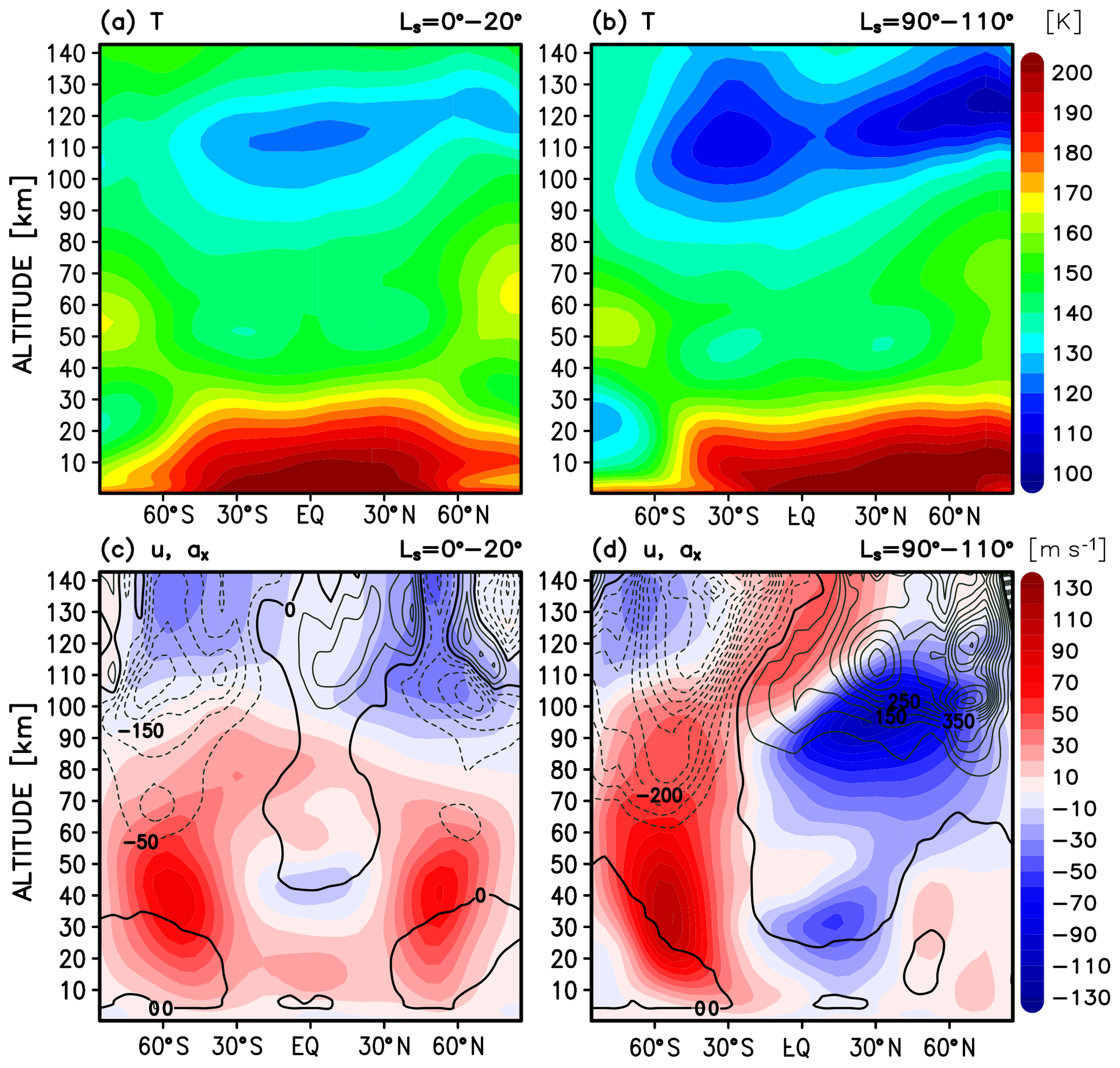
Figure 2 Altitude–latitude distributions of the mean zonal mean fields during vernal equinox and northern summer solstice (aphelion): (a) temperature (T) at equinox, (b) temperature (T) at solstice, (c) zonal wind u (color shaded) and zonal GW drag (acceleration/deceleration) a_x (contour lines), and (d) zonal wind u (color shaded) and zonal GW drag a_x (contour lines). The fields are averaged over L_s=0–20^∘ (42 sols) for vernal equinox and over L_s=90–110^∘ (44 sols) for the Northern Hemisphere summer period. Temperature is in units of K, the zonal wind is in m s⁻¹, and the zonal GW drag is in m s⁻¹ sol⁻¹. Red and blue shadings in the zonal wind plot represent the easterly (westward) and westerly (eastward) wind systems. Dashed and solid lines for the drag are for the easterly and westerly wave drags in intervals of 50 m s⁻¹ sol⁻¹.

Figure 1 presents the annual global means of the simulated temperature (T), GW-induced thermal heating–cooling rates (Q_GW), and CO₂ radiative cooling rates ($Q_{{\mathrm{CO}}_{\mathrm{2}}}$) for experiments EXP0 (dashed line) and EXP1 (solid line). The left panel demonstrates that inclusion of GW effects cools down the upper atmosphere at all altitudes above 60 km in a global sense; e.g., the temperature in the mesosphere above 100 km is lower by ∼10 K. Note that this change includes both thermal and dynamical influence of GWs. The thermal one is due to GW-induced heating/cooling rates, while the dynamical channel encompasses the temperature field response to acceleration/deceleration of the large-scale wind by small-scale GWs. Here, it is not our goal to explore the two channels in more detail. More important within the context of this paper is to demonstrate the appreciable net cooling effect of GWs.

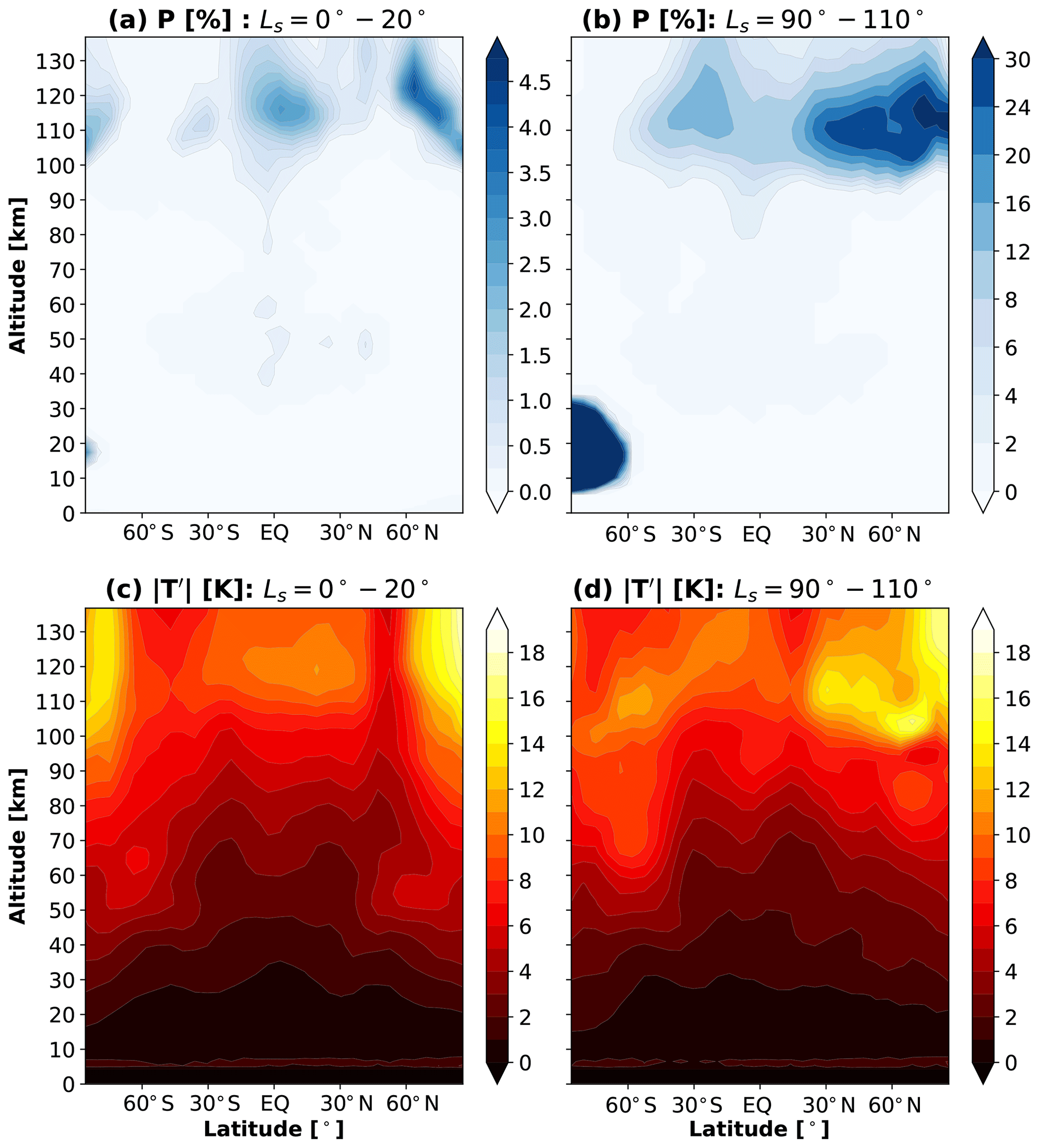
Figure 3 Altitude–latitude distributions of mean zonal mean cloud probability and gravity wave effects: (a) cloud probability (P) at equinox, (b) cloud probability at solstice, (c) gravity-wave-induced temperature fluctuations ($\left|T^{\prime }\right|=T_{\mathrm{GW}}^{\prime }$) at equinox, and (d) gravity-wave-induced temperature fluctuations at solstice. The fields are averaged over a period of L_s=0–20^∘ (42 sols) for vernal equinox and over L_s=90–110^∘ (44 sols) for Northern Hemisphere summer solstice seasons, i.e., in the same manner as the data presented in Fig. 2. Temperature fluctuations are in units of K and the probability is expressed in terms of percentage.

Figure 1b shows that CO₂ cooling is present at nearly all altitudes in the middle atmosphere, and peaks at more than −80 K sol⁻¹ around 90 km, steeply decreasing above. By contrast, GW cooling rates increase with altitude, exceeding that of CO₂ in the upper mesosphere and lower thermosphere, and peak at −80 K sol⁻¹ at 140 km. Around the mesopause and lower thermosphere, GWs cool down the atmosphere by ∼5–8 % (Fig. 1c). It is also seen that the GW-induced effects modulate the CO₂ cooling via changes in the background temperature: CO₂ cooling is up to 60 % weaker in the run with GWs. In the rest of the paper, we present the results of simulations that include GW effects (EXP1).

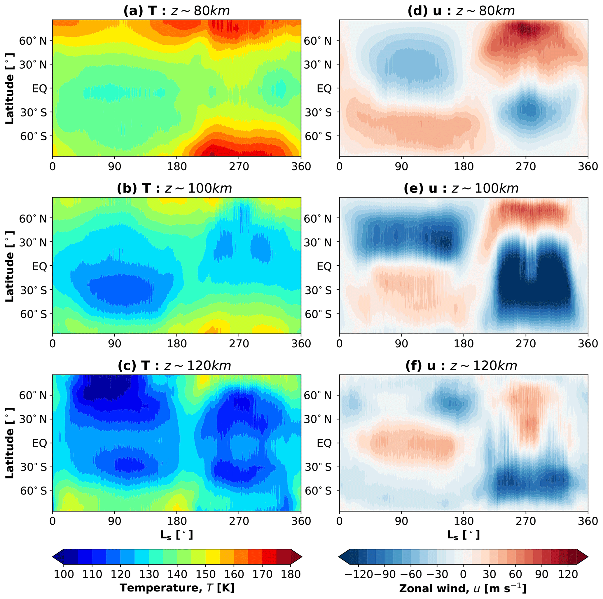
Figure 4 Seasonal variations of mean (i.e., daily and zonally averaged) atmospheric fields. (a) Temperature (T) at 80 km, (b) T at 100 km, (c) T at 120 km, (d) zonal wind (u) at 80 km, (e) u at 100 km, and (f) u at 120 km. Temperature is in K and the zonal wind is in m s⁻¹. Red/blue shadings for the wind represent eastward/westward winds. A Martian year has about 669 sols, which is plotted in terms of solar longitude L_s (in degrees) from L_s=0 to 360^∘. $L_{\mathrm{s}}=\mathrm{0}{}^{\circ }$ marks the vernal equinox in the Northern Hemisphere. $L_{\mathrm{s}}=\mathrm{90}{}^{\circ }$ and $L_{\mathrm{s}}=\mathrm{270}{}^{\circ }$ are aphelion and perihelion seasons, respectively.

Figure 2 illustrates the altitude–latitude distributions of the zonal mean temperature and wind for two characteristic seasons: the vernal equinox (averaged over 42 sols corresponding to L_s=0–20^∘, left panels) and the aphelion solstice (44 sol average, L_s=90–110^∘, right panels). The simulated temperatures below ∼70–80 km are in good agreement with observations, where systematic satellite measurements are available (Smith, 2008). The coldest temperatures on Mars (favoring CO₂ condensation) are near the mesopause. During the equinox, the minimum of 120 K is over the Equator. At the aphelion season, the mesopause is colder and the temperature minimum shifts to the summer hemisphere. This behavior is closely related to the wind distributions. It is seen that, in both seasons, zonal jets reverse their directions near the mesopause. The similar phenomenon is well known in the mesosphere and lower thermosphere of Earth, and is caused by the deposition of zonal momentum (i.e., zonal drag) by GWs of lower atmospheric origin (of up to −250 m s⁻¹ sol⁻¹ in this case), as demonstrated by the black contour lines. During the Northern Hemisphere summer solstice, the asymmetry between the two hemispheres is significant. Easterly and westerly jets dominate in the northern summer and southern winter hemispheres, respectively, with the middle atmospheric jets extending higher up and reversing their directions between 110 and 120 km due to zonal GW drag acting against the mean winds. The zonal mean drag increases from ±50 m s⁻¹ to $\pm \sim \mathrm{1000}$ m s⁻¹ sol⁻¹ from the mesosphere to the lower thermosphere, with relatively asymmetric distribution between hemispheres. The drag of similar magnitudes has been inferred from aerobraking data in the Martian lower atmosphere (Fritts et al., 2006).

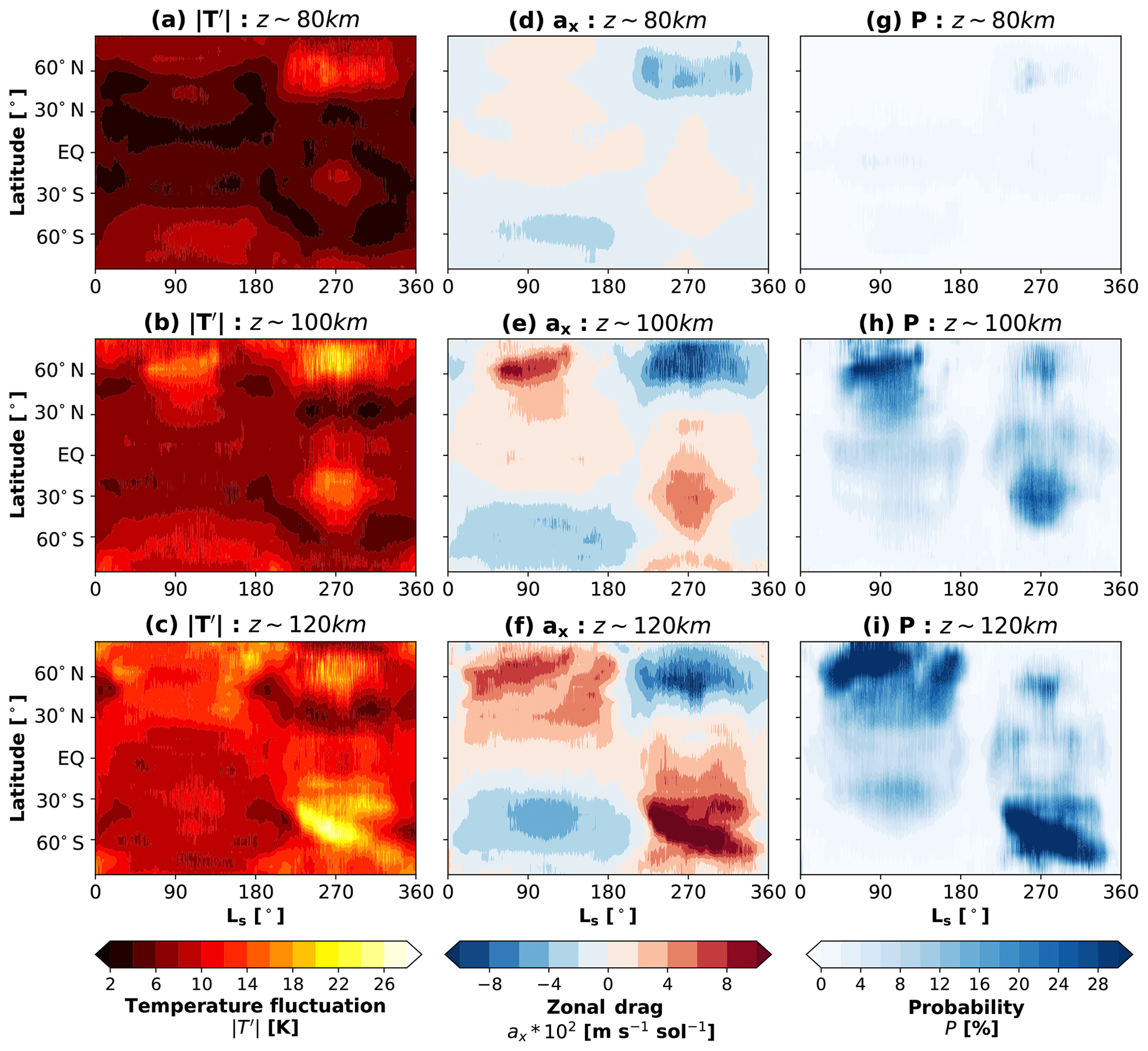
Figure 5 Seasonal variations of cloud formation probability, GW drag, and GW-induced temperature fluctuations: (a) GW-induced temperature fluctuations ($\left|T^{\prime }\right|$) at 80 km, (b) $\left|T^{\prime }\right|$ at 100 km, and (c) $\left|T^{\prime }\right|$ at 120 km, (d) GW zonal drag (a_x) at 80 km, (e) a_x at 100 km, (f) a_x at 120 km, (g) cloud formation probability (P) at 80 km, (h) P at 100 km, and (i) P at 120 km. Probabilities are in percentage; zonal drag is in m s⁻¹ sol⁻¹, and temperature fluctuations are in K. In the drag plots (d–f), red/blue represents eastward/westward GW drag. Presented model data are in terms of daily and zonal averages. Note that the zonal drag is plotted in 200 m s⁻¹ sol⁻¹ intervals. $L_{\mathrm{s}}=\mathrm{0}{}^{\circ }$ marks the vernal equinox in the Northern Hemisphere.

Figure 3 demonstrates that the probability P of CO₂ cloud formation is strongly determined by the mean temperature. It is seen that the saturation conditions for clouds are more likely to be met during the solstice than the equinox. Specifically, the cloud formation can occur in ∼1 % of the time in the equatorial mesosphere during the equinox. Higher up at around 120 km, the cloud formation probability increases and reaches 4.5 % with larger values found at the northern high latitudes. During the solstice, the probability P is larger in all atmospheric regions. In particular, a very strong cloud formation is seen in the winter polar lower atmosphere (Fig. 3b), which, however, is not the focus of this paper. In the upper atmosphere, the peak values of P exceed 30 % between 100 and 120 km in the Northern Hemisphere at middle and high latitudes. A closer examination of Figs. 2 and 3 reveals that the distributions of P and mean temperature are not identical. GW-induced fluctuations $\left|T^{\prime }\right|$, which are a measure of GW activity, also contribute to CO₂ supersaturation, especially at low to middle latitudes of the middle atmosphere in both seasons and in high-altitude polar regions. Overall, large GW-induced temperature fluctuations prevail above 100 km up to 140 km, primarily located over the Equator and at high latitudes of both hemispheres.

4 Seasonal variation of the mean fields

We next investigate the seasonal variations of the simulated temperature and wind in more detail by focusing on three representative altitudes in the mesosphere and lower thermosphere: 80, 100, and 120 km. There are too few observations at these altitudes to date to validate the simulations. The exception is the temperature at ∼80 km (Fig. 4a), which can be directly compared to retrievals from Mars Climate Sounder (MCS) onboard Mars Reconnaissance Orbiter (MRO) (Sefton-Nash et al., 2013). Both observations and simulations demonstrate a relative symmetry with respect to the equatorial distributions during equinoxes ($L_{\mathrm{s}}=\mathrm{0}{}^{\circ },L_{\mathrm{s}}=\mathrm{180}{}^{\circ }$). The lowest and highest temperatures occur in the Southern Hemisphere during winters and summers, respectively. The model generally reproduces the observed temperature well, except that it overestimates it in the Southern Hemisphere winter by up to 20 K. Alternating with seasons, zonal winds at ∼80 km represent an extension of the lower and middle atmosphere jets formed as a consequence of the Coriolis force acting on the summer-to-winter meridional circulation cell.

In the upper mesosphere (100 km, Fig. 4b, e) the simulated temperature and wind show variations similar to that at 80 km, but with noticeably colder temperatures. Around the mesopause (120 km, Fig. 4c, f), the simulated seasonal variations differ significantly from those in the mesosphere. It is seen that the coldest temperatures of down to 90–100 K are found around the summer high latitudes at solstices, and the temperature distributions are hemispherically less symmetric. The summer high-latitude hemispheres are remarkably different. Polar temperatures fall down to 90 K in the summer hemisphere at the aphelion and to 115 K at the perihelion. The zonal winds reverse their directions at 120 km, which is especially well seen during the aphelion season. During other seasons, the simulated winds demonstrate a significant weakening as compared to distributions in the mesosphere. The latter is primarily attributed to the GW drag, which we present next along with GW-induced temperature fluctuations.

5 Seasonal variation of gravity wave activity and probability of CO₂ ice clouds

Parameterized GW-induced temperature fluctuations ($\left|T^{\prime }\right|$), GW drag (a_x), and probability of cloud formation (P) are studied next in Fig. 5 in the same manner as temperature and zonal winds are presented in Fig. 4. Overall, the seasonal variations of the parameterized GW-induced temperature fluctuations, which are created by GW harmonics that survived propagation from the lower atmosphere, depend on the assumed wave sources and on filtering by the underlying mean winds. In the mesosphere (80 km, Fig. 5a), the fluctuations of up to 16 K enhance at middle to high latitudes and during the solstices with slightly larger magnitudes during winters. The middle column of Fig. 5 shows the seasonal variations of the zonal GW drag, which is largely determined by the background winds below presented in Fig. 4 and characterizes the rate of change in GW momentum fluxes with height. It is seen that it is directed mainly against the mean flow throughout the mesosphere. Finally, the probability P of cloud formation is plotted in the rightmost column of Fig. 5. A continuous presence of P of up to 2–4 % is seen around the Equator at 80 km nearly throughout the entire Martian year. After the northern summer hemisphere solstice (aphelion), regions of cloud formation gradually expand to lower latitudes ($\pm \mathrm{30}{}^{\circ }$), resembling a fork-like structure, in some level of agreement with Sefton-Nash et al. (2013)'s observations. During southern winter solstice, the probability of cold pocket formation is somewhat present around middle latitudes. There is some degree of correlation between the cloud formation probability and GW activity represented as fluctuations and drag.

In the upper mesosphere (100 km, middle row), GW-induced temperature fluctuations increase, along with the GW drag imposed on the mean circulation, and the cloud formation probability demonstrates a more definitive correlation with the GW activity during all seasons. Cold pockets occur more frequently at middle and high latitudes (P∼16 %–20 %), exceeding the equatorial cloud probability rate. Around the mesopause, GW-induced fluctuations increase further, maximizing at middle and high latitudes with values of up to 26 K during both aphelion and perihelion. The probability P increases to more than ∼30 % correspondingly.

6 Discussion

As mentioned in the description of the model, the CO₂ condensation/sublimation scheme employed in the MPI-MGCM is able to resolve CO₂ ice formation and annihilation when temperature in a grid point crosses the condensation threshold. In our simulations, there were very few occurrences of such clouds in the mesosphere above 60 km to offer reliable statistics. Inclusion of GW effects leads, generally, to colder simulated temperatures, which provide favorable conditions for cloud formation. This cooling in the mesosphere is mainly produced via the dynamical channel due to GW-induced changes in the winds that affect temperature through the thermal wind relation, rather than via the thermal channel due to direct heating/cooling by dissipating GW harmonics. The latter clearly transpires in experiments with thermal effects of the parameterized waves turned on and off (not shown). The direct thermal effects of GWs increasingly grow with height and become important near the mesopause and above.

The vast majority of studies report on cloud observations in the Martian mesosphere below ∼80 km. Sefton-Nash et al. (2013) analyzed data from Mars Climate Sounder (MCS) onboard the Mars Reconnaissance Orbiter (Graf et al., 2005; Zurek and Smrekar, 2007) (MRO) during dayside and nightside local times over 2 Martian years and provided a global picture of high-altitude clouds. They found out that the distribution of clouds over latitude and season does not appear to vary between each Martian year and that clouds occurred more often in low latitudes during the aphelion season and concentrated around two mid-latitude bands during perihelion. Using two different observational modes, Sefton-Nash et al. (2013) showed that the latitudinal distributions of clouds varied little between the different local times in the second half of the year. It must be noted that Sefton-Nash et al. (2013) could not discriminate between CO₂ and water clouds. The majority of positively identified CO₂ cloud observations took place in the first half of the year, with only a few detections in the second half. On the other hand, water ice clouds usually do not extend higher than ∼40 km except during perihelion, when they rise to 60–65 km. Therefore, all clouds observed above 70 km are likely not water ice clouds. The question regarding the nature of these detected clouds is still open. Our simulations illustrate that favorable conditions for CO₂ condensation in the mesosphere exist in low latitudes throughout the year (Fig. 5g). This is because the mean temperature is lowest around the Equator at all seasons (Fig. 4a), while GW-induced temperature fluctuations are contrastingly small (Fig. 5a). The model also predicts a higher probability of cloud formation in middle latitudes of the summer hemisphere during both solstices.

It is observationally challenging to determine the precise altitude of CO₂ ice clouds and there are intrinsic limitations of the retrieval algorithms associated with CO₂ cross sections (Määttänen et al., 2013). Nevertheless, our modeling results can qualitatively be compared with Sefton-Nash et al. (2013)'s analysis of the seasonal variation of Martian high-altitude clouds. The observations show that during Northern Hemisphere summer, clouds formed in the mesosphere more rarely than during perihelion and were located mainly around the Equator. Previous analysis of the data from the Thermal Emission Spectrometer (TES) onboard the Mars Global Surveyor (MGS) (Clancy et al., 2007) also indicated that cloud occurrences were confined to a narrow latitude sector of $\pm \mathrm{15}{}^{\circ }$ during the aphelion season (L_s=30–150^∘). In agreement with observations, our simulations show higher probabilities of cloud formation in low latitudes throughout all seasons (Fig. 5g). The latter is simply a consequence of the temperature minimum near the equatorial mesopause. The model reproduces more favorable conditions for CO₂ condensation in the mid-latitude regions during wintertime. It agrees with observations in that mesospheric clouds occur more frequently during perihelion (Fig. 5g). Cold pockets with supersaturated temperatures occur in the model only in less than 10 % of the time at ∼80 km, but their probabilities grow with height. At 100 km, maxima of P of up to ∼18 % are seen in middle latitudes of the summer hemispheres (Fig. 5h), while higher up at ∼120 km these maxima exceed ∼30 % and shift poleward (Fig. 5i). Such behavior is due to growth with height amplitudes of GWs and the associated temperature fluctuations (Fig. 5a–c). The shift of maxima of cloud probabilities first to middle and then to high latitudes is caused by the cold anomaly of the mean temperature, which is induced by GWs in the mesosphere. The similar GW-induced cold summer mesopause anomaly is well known in the atmosphere of Earth (Garcia and Solomon, 1985).

There are certain disagreements between the modeled cloud formation probabilities and existing observations at high altitudes (80 km and above). In particular, the dayside observations of Sefton-Nash et al. (2013) demonstrate a greater symmetry with respect to the equatorial distribution of CO₂ clouds during the first part of the year. They do not show a “pause” near the equinox around $L_{\mathrm{s}}=\mathrm{180}{}^{\circ }$, which is clearly seen in Fig. 5h, f. It is worth noting that the superposition of the simulated patterns at 80 and 100 km is close to the superposition of the observed night and day patterns (Sefton-Nash et al., 2013) attributed to the 80 km altitude. Finally, there is no statistically significant observational support for the predicted cloud formation probability above 80 km. We, therefore, discuss possible reasons and shortcomings of the modeling methodology.

One source of uncertainty in our simulations is the assumed degree of supersaturation, which is currently 35 % based on previous experimental constraints (Glandorf et al., 2002). However, a variable with a height supersaturation threshold is possible, which could modulate P in our numerical experiments. This variable threshold may reflect the microphysics of cloud formation, which implies an existence of nuclei and strong dependence on their sizes. It is likely that the existence of cold pockets (the necessary condition for cloud formation) is far from sufficient for clouds to form, especially in the upper atmosphere. Thus, the lack of nuclei in the upper atmosphere may prevent cloud formation. If formed, ice particles must be small (being of submicron size) and clouds are too thin to be previously detected.

In all our simulations, only probabilities of GW-induced clouds were calculated and, thus, no radiative effects of such clouds were taken into account. Such radiative feedback has been considered, for example, in the work by Siskind and Stevens (2006) in the Earth context. However, one can expect that, given that IR CO₂ and GW thermal effects together dominate the energy budget of the mesosphere (Medvedev et al., 2015), secondary radiative processes are likely to play a relatively minor role in the cloud formation by producing local modulations of temperature. A more comprehensive examination of the radiative feedback processes in the Martian environment would require a two-way coupling between microphysics and small- and large-scale dynamics. Interestingly, using a one-dimensional radiative–convective model, Mischna et al. (2000) demonstrated that the lower atmospheric CO₂ clouds have a potential to produce an additional cooling of the Martian surface by reflecting the incoming solar radiation. A further source of uncertainty is the use of a one-dimensional atomic oxygen profile, which may affect neutral temperatures.

An obvious candidate for explaining mismatches between the modeling and observations is the specification of sources in the GW parameterization. In the simulations, we assumed a globally uniform and constant-with-time distribution of GW momentum fluxes. The magnitudes of the fluxes were chosen from observations to capture the “background” effect of small-scale waves, as described in detail in our earlier works (Medvedev et al., 2011a, b). Recently, using a high-resolution Martian GCM, Kuroda et al. (2015, 2016) have shown a strong seasonal and latitudinal variation of GW momentum fluxes in the lower atmosphere and, as a result, significant variations of GW-induced activity in the middle atmosphere. Constraining wave sources is a logical next step in model development, which can potentially improve simulations of clouds.

Finally, other limitations in the model can result in imperfections with the simulated mean fields and, as a consequence, erroneous estimates of cloud formation probability P. The reviewer suggested that accounting for radiative effects of water clouds and for a more realistic dust scenario (mainly associated with its vertical distribution) may affect the simulated P. These and other undertaken paths of MGCM sophistication, like self-consistent modeling of water and aerosol cycles, can potentially bring observations and simulations of CO₂ clouds closer.

7 Summary and conclusions

We presented simulations with the Max Planck Institute Martian General Circulation Model (MPI-MGCM) (Medvedev et al., 2013), incorporating a whole atmosphere subgrid-scale gravity wave (GW) parameterization of Yiğit et al. (2008), and of distributions of mean fields, GW effects, and cloud formation probabilities over 1 Martian year, assuming a multi-year averaged observed dust distribution with major dust storms removed. Model results are compared to a run without the subgrid-scale effect included.

Inclusion of effects of small-scale GWs facilitates CO₂ cloud formation in two ways. First, they cool down the upper atmosphere globally and, second, they create excursions of temperature well below the CO₂ condensation threshold in some parts of the middle atmosphere. The main findings of this study are as follows.

1. GWs lead to ∼9 % colder global annual mean temperatures and even stronger temperature drops locally. Global annual mean GW-induced cooling of −30 K sol⁻¹ is comparable with that of radiative transfer by CO₂ molecules around 100 km, and exceeds it above, reaching −80 K sol⁻¹ around 140 km. GW-induced effects modulate the CO₂ cooling via changes in the background temperature.

2. Simulations reveal strong seasonal variations of GW effects in the upper mesosphere and lower thermosphere with solstitial maxima: eastward GW drag peaks during the summer solstices and westward GW drag maximizes around the winter solstices with up to ±1000 m s⁻¹ sol⁻¹.

3. Around the mesopause, GW-induced temperature fluctuations $\left|T^{\prime }\right|$ can exceed 20 K and the ice cloud formation probability (P) can be greater than 20 % locally.

4. Overall, GW temperature fluctuations substantially correlate with the cloud formation probability, in particular at middle and high latitudes in the upper mesosphere and mesopause region during all seasons.

5. Cloud formation exhibits strong seasonal variations larger than 30 %, with summer solstitial maxima at high latitudes in the mesosphere and around the mesopause.

6. The simulated seasonal variations of cloud probabilities in the mesosphere are in reasonable agreement with previous detections of two distinct mesospheric types of clouds, i.e., equatorial and mid-latitude clouds.

This study has shown that accounting for GW-induced temperature fluctuations in the Martian GCM reproduces supersaturated cold temperatures in the upper mesosphere throughout all seasons. GWs maintain globally cooler air, which is necessary for ice cloud formation, and help to explain some features of the observed seasonal behavior of high-altitude CO₂ ice clouds. Owing to GW-induced globally colder temperatures and local temperature fluctuations, high-altitude clouds can form from the upper mesosphere to the mesopause region, and occasionally even slightly above the mesopause. We conclude that GW dynamical and thermal effects not only maintain the colder Martian mesosphere and lower thermosphere, but also significantly contribute to the specific features of the observed high-altitude clouds and their seasonal variations.

This study also puts forward new questions. Are our results concerning shaping the seasonal behavior of ice clouds model-specific? Can CO₂ clouds form at altitudes above the mesopause, as the simulations predict? How does the microphysics of cloud formation modify these predictions? Further systematic modeling and observational efforts have to be performed in order to address these open questions.

Appendix A: Martian parameters and seasons

Mars demonstrates in terms of planetary parameters some similarities as well as differences to Earth as summarized in Table A1.

In planetary atmospheres, one “sol” refers to the duration of a solar day on Mars. The length of a day is longer on Mars than on Earth. One Martian sol is about 24 h and 39 min (i.e., 24.65 h), and thus slightly longer than an Earth day. One Martian year is 687 days long or 669 Martian sols. Due to different eccentricities of Mars and Earth, their distance can vary significantly over the course of their orbital motion around the Sun. Martian seasons are described by the solar longitude L_s. In our modeling, by convention, L_s=0 vernal equinox, $L_{\mathrm{s}}=\mathrm{90}{}^{\circ }$ is Northern Hemisphere solstice (aphelion), $L_{\mathrm{s}}=\mathrm{180}{}^{\circ }$ is autumnal equinox, and $L_{\mathrm{s}}=\mathrm{270}{}^{\circ }$ is Northern Hemisphere winter solstice (perihelion).

Table A1 Some key planetary parameters of Earth and Mars.

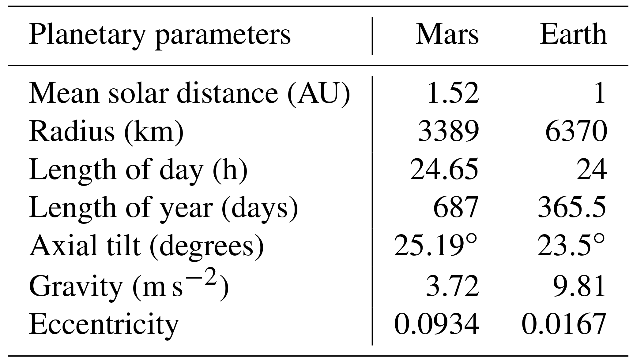
The solar distance designates the average distance from the Sun, given in terms of AU ∼150 million km. The axial tilt, or obliquity of the orbit, is measured with respect to the orbital plane. One solar day on Mars is referred to as one sol.