Long-term trends in stratospheric ozone, temperature, and water vapor over the Indian region

We have investigated the long-term trends in and variabilities of stratospheric ozone, water vapor and temperature over the Indian monsoon region using the long-term data constructed from multi-satellite (Upper Atmosphere Research Satellite (UARS MLS and HALOE, 1993–2005), Aura Microwave Limb Sounder (MLS, 2004–2015), Sounding of the Atmosphere using Broadband Emission Radiometry (SABER, 2002–2015) on board TIMED (Thermosphere Ionosphere Mesosphere Energetics Dynamics)) observations covering the period 1993–2015. We have selected two locations, namely, Trivandrum (8.4^∘ N, 76.9^∘ E) and New Delhi (28^∘ N, 77^∘ E), covering northern and southern parts of the Indian region. We also used observations from another station, Gadanki (13.5^∘ N, 79.2^∘ E), for comparison. A decreasing trend in ozone associated with NO_x chemistry in the tropical middle stratosphere is found, and the trend turned to positive in the upper stratosphere. Temperature shows a cooling trend in the stratosphere, with a maximum around 37 km over Trivandrum (−1.71 ± 0.49 K decade⁻¹) and New Delhi (−1.15 ± 0.55 K decade⁻¹). The observed cooling trend in the stratosphere over Trivandrum and New Delhi is consistent with Gadanki lidar observations during 1998–2011. The water vapor shows a decreasing trend in the lower stratosphere and an increasing trend in the middle and upper stratosphere. A good correlation between N₂O and O₃ is found in the middle stratosphere (∼ 10 hPa) and poor correlation in the lower stratosphere. There is not much regional difference in the water vapor and temperature trends. However, upper stratospheric ozone trends over Trivandrum and New Delhi are different. The trend analysis carried out by varying the initial year has shown significant changes in the estimated trend.

Keywords. Atmospheric composition and structure (middle atmosphere – composition and chemistry; troposphere – composition and chemistry) – meteorology and atmospheric dynamics (climatology)

1 Introduction

Ozone and water vapor are two potent greenhouse gases in the atmosphere. Over the tropical regions, stratospheric ozone depletion is not a critical problem but tropospheric ozone is a serious issue. The absorption of solar radiation by ozone in the Hartley, Huggins, and Chappuis bands is the major reason for the heating of the middle and upper stratosphere. Apart from this, the two strong bands at 9.6 and 15 µm in the infrared region cool the upper atmosphere and cause the greenhouse effect in the lower atmosphere (Wang et al., 1980). A large number of ozone and temperature observations are available at different stations all over the globe (compared to water vapor, methane, nitrous oxide, etc.). These observations show that the industrial revolution has changed the ozone precursors in the troposphere through anthropogenic sources, and thereby the radiative forcing (∼ 0.40 ± 0.20 W m⁻²) has increased significantly due to ozone (IPCC, 2013). Detection and estimation of long-term changes in the atmospheric constituents and parameters by different statistical methods will show the natural and anthropogenic effects on the climate change. Only long-term trend observations can give reliable evidence of the current state of the atmosphere and the effect on climate and ecosystems. They are essential for the numerical simulations/climate modeling to predict the future state of the atmosphere.

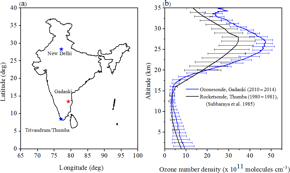
Figure 1 (a) Map showing the Indian subcontinent with Trivandrum, Gadanki, and New Delhi locations. (b) Comparison of rocketsonde ozone profiles (black) observed over Trivandrum during 1980–1981 with ozonesonde profiles (blue) observed over Gadanki during 2010–2014.

In India from 1971 onwards, every fortnight ozonesonde launchings have been conducted by the India Meteorological Department (IMD) from three stations (Mani and Sreedharan, 1973) namely Trivandrum (8.4^∘ N, 76.92^∘ E), Pune (18.53^∘ N, 73.85^∘ E), and New Delhi (28.6^∘ N, 77.2^∘ E). Rocketsonde ozone observations from Trivandrum were conducted during 1980–1981 to study the day to night changes of ozone at different levels in the tropical stratosphere and the lower mesosphere. Figure 1a shows the location of Thumba/Trivandrum along with New Delhi. Long-term trends in tropospheric ozone over the Indian region have been studied by Saraf and Beig (2004) using the ozonesonde observations from the three IMD stations for a period of 30 years, from 1971 to 2001. They reported no statistically significant trend over Trivandrum but a significant positive trend throughout the troposphere over New Delhi and in the upper troposphere over Pune. Fadnavis et al. (2013) also reported a positive trend (0.5–2 % decade⁻¹) in ozone in the upper troposphere over Pune and New Delhi. The increasing trend in ozone is attributed to the increase in the NO_x concentration in the upper troposphere. They also found a positive trend in ozone between 100 and 30 hPa and thereafter a negative trend up to 10 hPa.

Regular launching of ozonesonde every fortnight from National atmospheric Research Laboratory (NARL), Gadanki (13.5^∘ N, 79.2^∘ E), has been conducted from 2011 onwards (Akhil Raj et al., 2015), and a special campaign (consisting of seven launchings) was conducted during the 2010 annular eclipse (Ratnam et al., 2011). A very good comparison between Gadanki ozonesonde and Sounding of the Atmosphere using Broadband Emission Radiometry (SABER), Microwave Limb Sounder (MLS), and ERA-Interim has been found above 20 km altitude (Akhil Raj et al., 2015). To visualize the changes in ozone vertical distribution in the last 3 decades, we compared Thumba rocketsonde ozone profiles (Subbaraya et al., 1985) with ozonesonde profiles observed from Gadanki, which is shown in Fig. 1b. There were 19 rocketsonde launchings during 1980–1984. Though most of the rocket measurements start from 16 km, only ozone concentration data corresponding to 20 km and above are considered in the present study due to large variation from one measurement to the other in the 16–20 km range. For altitudes below 20 km ozonesonde measurements from IMD, Trivandrum (8.5^∘ N, 76.9^∘ E) observations are used. In the initial analysis, comparison of 1980s observations with those of the recent decade shows a significant increase in the ozone concentration at the ozone peak altitude together with the rise in the altitude of ozone minima in the upper troposphere. Our primary objective is to investigate the trends in the stratospheric ozone over India and understand the regional dependence on the trends. Along with ozone trends we also estimated the water vapor and temperature trends.

Stratospheric water vapor cools the stratosphere and causes warming of the surface through the greenhouse effect (de Forster and Shine, 1999). The process of stratospheric feedback increases stratospheric water vapor, which leads to additional warming (Dessler et al., 2013). Since solar insolation at the tropical regions is higher than at midlatitudes and polar latitudes, this feedback would have more effect on the tropical climate. Though the concentration of water vapor is low in the upper troposphere and the stratosphere, it can significantly influence the climate (Held and Soden, 2000). It is well known that the tropopause temperature controls the seasonal cycle of water vapor entering the lower stratosphere (Mote et al., 1996). The in situ production of water vapor by the oxidation of methane (CH₄) contributes to the observed water vapor in the stratosphere apart from the transport from the upper troposphere.

Global mean cooling of the stratosphere is observed, and evidence points towards anthropogenic activities as having an impact on climate (Kishore et al., 2014, and references there in). We have estimated the long-term trends in temperature along with ozone and water vapor. Several trace gases have strong absorption bands in the infrared (IR) region (5 to 20 µm), which contributes to the greenhouse effect by enhancing the opacity of the atmosphere. Stratospheric temperature perturbation by the IR cooling due to the increase in trace gases alters the middle stratospheric chemistry via temperature-dependent reaction rates (Ramanathan et al., 1985, and references there in). Ozone is one of the kinds of chemicals (gases) that have temperature-dependent reactions; hence this will lead to the perturbation of stratospheric ozone. New stratosphere-resolving general circulation models and chemistry-climate models have predicted the strengthening of the Brewer–Dobson circulation (BDC) in response to climate change induced by greenhouse gases (Butchart, 2014; Butchart and Scaife, 2001). The BDC has an important role in determining many aspects, such as the thermodynamic balance of the stratosphere, the transport of ozone and other chemical species, and the entry of water vapor into the stratosphere. The strengthening of the BDC also causes the transport of tropical lower stratospheric ozone to midlatitudes and polewards. For the present study we considered 23 years of ozone mixing ratio data by combining observations from the Microwave Limb Sounder (MLS) (1993–1999), the Halogen Occultation Experiment (HALOE) (1993–2005) on board the Upper Atmosphere Research Satellite (UARS), and the Earth Observing System (EOS) Microwave Limb Sounder (MLS) on board the Aura spacecraft (2004–2015). HALOE (1993–2005) and SABER (2002–2015) temperature data are used for the estimation of temperature trends. Along with this, UARS HALOE (1993–2005) and MLS (2004–2015) on-board Aura water vapor data are also used for estimating the trends in the water vapor mixing ratio. To investigate the regional dependence of the trends, we considered two locations within India, namely Trivandrum, a tropical station, and New Delhi, a subtropical station.

2 Database and methods

2.1 HALOE and MLS on board UARS

HALOE is a solar occultation instrument on board the UARS satellite that takes observations during limb viewing conditions (Russell et al., 1993) and gives 15 sunrise and sunset measurements per day. HALOE uses transmittance solar infrared radiations in the 2.45 to 10.04 µm range and measures O₃, HCL, CH₄, NO, NO₂, H₂O, aerosol extinction, and temperature versus pressure from 80^∘ S to 80^∘ N. However the 57^∘ inclination limits the majority of the observations to the higher latitudes, and the number of observations in the tropics and subtropics is lower when compared to higher latitudes. The altitude range of measurement is from 15 km to 60–130 km with a vertical resolution of ∼ 2 km or less depending on the channel. Ozone and water vapor profiles are retrieved from 9.852 and 6.605 µm transmission wavelengths, respectively. Temperature is retrieved from the atmospheric transmission measurements of the 2.80 µm CO₂ band. To avoid the influence of the Mount Pinatubo eruption in the observations, we used ozone, water vapor, and temperature observations from 1993 to 2005. Since the overpass of the satellite is not expected every day over a given location, we considered a 10^∘ × 20^∘ (lat × long) grid to make sure a reasonable number of observations is available over Trivandrum and New Delhi to generate statistics.

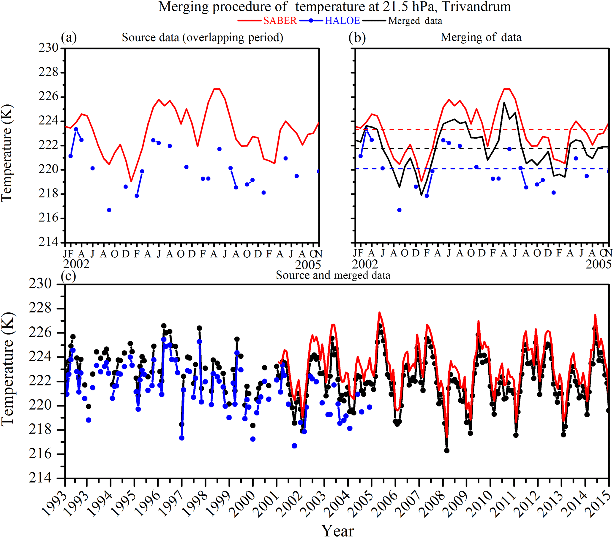
Figure 2 Merging procedure illustrated for temperature at 21.5 hPa over Trivandrum. (a) Monthly mean source data during overlapping period (January 2002–November 2005) for HALOE and SABER at 21.5 hPa over Trivandrum. (b) The merged product (black) resulting from the adjustment of source data to the mean reference indicated by black dashed line (mean of co-located HALOE and SABER data) along with source data. Blue and red dashed lines show the mean of HALOE and SABER during the overlapping period. (c) Final merged temperature by applying additive offset value to the source data during 1993–2015.

Ozone observations from MLS on board UARS during the time period of 1993 to 1999 are also used for the present study. The MLS retrieves ozone profiles from the calibrated microwave radiances in two separate bands, at frequencies near 205 and 183 GHz. A detailed description of UARS MLS ozone and other data products are available elsewhere (Froidevaux et al., 1996; Livesey, 2003). The MLS instrument measures in the microwave emission spectrum near 63, 205, and 183 GHz by three different radiometers. The instrument performs Earth's atmosphere limb scan from around 1 to 90 km tangent point altitude every 65.536 s, and this is known as one MLS major frame, which consists of 32 MLS minor frames. Due to the failure of the 183 GHz radiometer in mid-April 1993, we could not use the ozone and water vapor information from this channel. For the present study we made use of 205 GHz channel data from 1993 to 1999.

2.2 SABER on board TIMED

The SABER is one of the instruments on NASA's TIMED satellite launched on 7 December 2001. The TIMED satellite is at 625 km orbit with an orbital inclination 74.1^∘, and its period is ∼ 97 min. SABER scans the horizon with a 10-channel broadband limb scanning radiometer ranging from 1.2 to 17 µm wavelength. The ground station will provide approximately 2 km altitude resolution profiles of temperature, O₃, H₂O, and CO₂ along with other data products from the observed vertical horizon emission profile (Russell III et al., 1999). Temperature is retrieved from the atmospheric 15 µm CO₂ limb emission (García-Comas et al., 2008) and ozone on a daily basis in the middle and upper atmosphere from the 9.6 µm channel (Rong et al., 2009). For the present study we used version V2.0 temperature data obtained during the period from 2002 to 2015.

2.3 MLS on board EOS/Aura

Apart from the UARS HALOE, MLS (UMLS), and SABER, we have also utilized the data sets from the Earth Observing System (EOS) Microwave Limb Sounder (MLS) on board the Aura spacecraft (AMLS). AMLS is a second-generation follow-on experiment to the successful MLS instrument on UARS. AMLS measures several atmospheric species, cloud ice, temperature, and geopotential height. The instrument uses heterodyne limb radiometers to make simultaneous and continuous observations during day and night. The instrument observes the thermal emission from the atmospheric limb in broad spectral regions centered near 118, 190, 240, and 640 GHz and 2.5 THz (Waters et al., 2006). The instrument performs an atmospheric limb scan and radiometric calibration for all bands every 25 s. With a latitude coverage of 82^∘ N–82^∘ S for each orbit, AMLS retrieves profiles every 165 km along the suborbital track. In the present work we used version 3 ozone and water vapor data and version 4 nitrous oxide (N₂O) data over Trivandrum and New Delhi from 2004 to 2015.

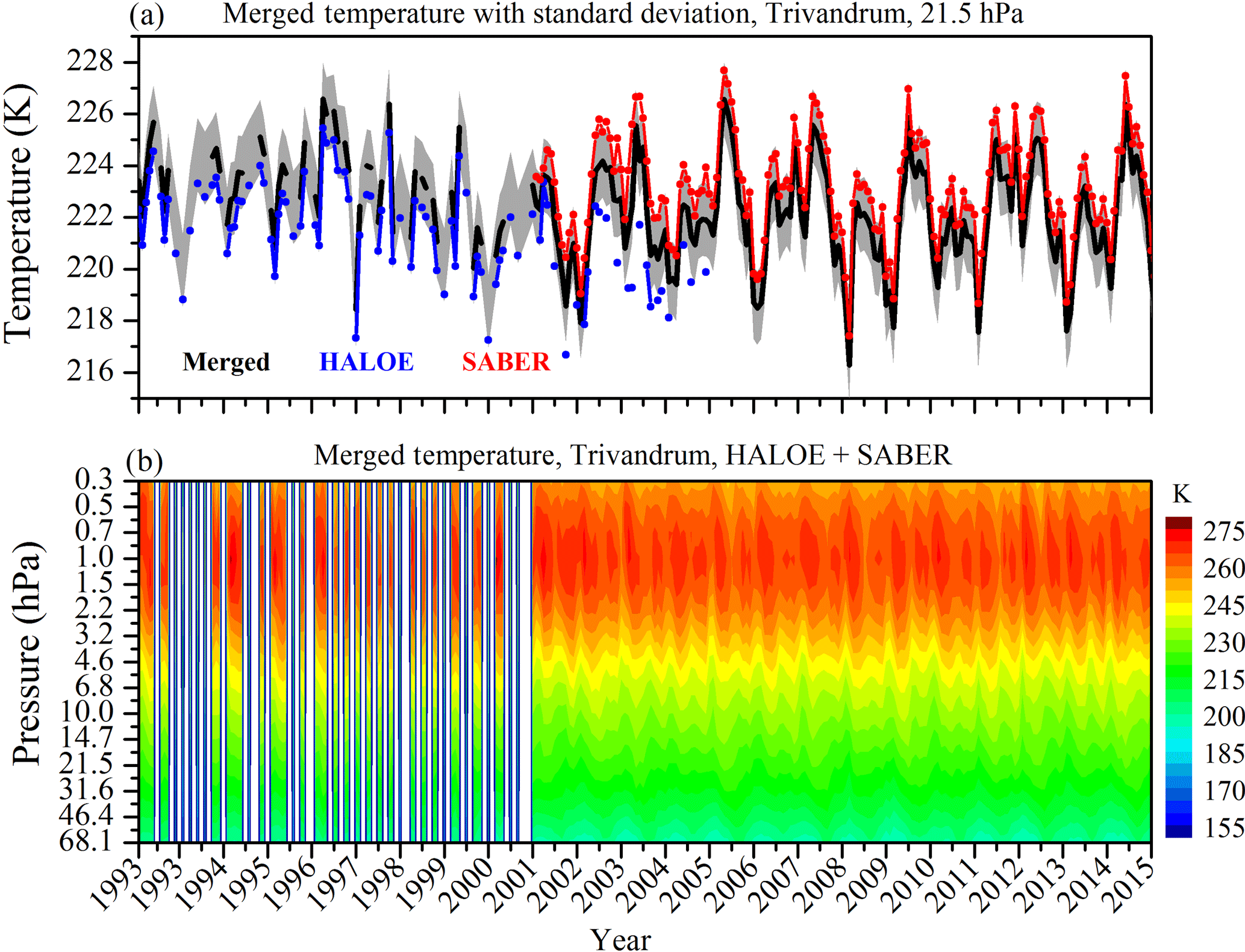
Figure 3 (a) Systematic error calculated from monthly mean temperature observations from HALOE and SABER over Trivandrum at 21.5 hPa with source data. (b) Contour of the temperature over Trivandrum from 1993 to 2015 after removing the bias.

2.4 Merging of satellite data

As different instruments on board the above-mentioned satellites are used and the time periods are not the same, they need to be suitably merged to obtain meaningful long-term trends. In order to accommodate the lower vertical resolution profiles from UMLS we have interpolated higher vertical resolution data into a standard pressure grid and the pressure grid as

$$\begin{array}{}\text{(1)}& {\displaystyle }p\left(i\right)=\mathrm{1000}\times {\mathrm{10}}^{-i/\mathrm{6}}\left(\text{hPa}\right),\end{array}$$

with i varying from 0 to a product-dependent top. Monthly mean temperature, ozone mixing ratio, and water vapor mixing ratio are used to produce merged data. We used a 10^∘ × 20^∘ grid to construct monthly mean data. We followed the method of Froidevaux et al. (2015) for merging the satellite data in the present work. Merging is done by computing average relative biases between the source data sets during the overlapping periods and then applying additive offsets to each source of data to adjust them to a common reference to remove relative biases. Figure 2 illustrates the merging procedure of temperature at 21.5 hPa over Trivandrum. HALOE and SABER temperature data are used for producing merged temperature from 1993 to 2015. Figure 2a shows the source data from HALOE (blue) and SABER (red) during the overlapping period from January 2002 (SABER data start) through November 2005 (HALOE data end). Figure 2b illustrates the merged product (black) during the overlapping period resulting from the adjustment of HALOE and SABER to the mean reference (black dashed line), the average of both time series when both values exist. We first obtained the merged data via

$$\begin{array}{}\text{(2)}& {\displaystyle }{m}_{\mathrm{1}}\left(i\right)=(\mathrm{1}/\mathrm{2})\left(y_{\mathrm{2}}\right(i)+y_{\mathrm{2}}(i\left)\right),\end{array}$$

and with this we have calculated the offset for y₁(i) and y₂(i) as

$$\begin{array}{}\text{(3)}& {\displaystyle }(\mathrm{1}/(\mathrm{2}{n}_{\mathrm{12}}\left)\right)\sum \left(y_{\mathrm{1}}\right(i)-y_{\mathrm{2}}(i\left)\right),\end{array}$$

where n₁₂ is the number of overlapping data points between the two time series. Since the number of collocating points is much lower over the tropics, we followed another method instead of directly averaging the data points. The offset is calculated using Eq. (3), where the gap of y₂(i) (using HALOE data) is replaced with the mean of overlapping data to improve the offset value. This calculated offset is applied to the data sets and the average is calculated to obtain the merged data during the overlapping period. Figure 2c shows the merged data for the full-time period (1993 to 2015). The water vapor merged data product is made up of HALOE and AMLS observations following the same method (as temperature).

We used ozone data from UMLS (1993–1999), HALOE (1993–2005), and AMLS (2004–2015) for producing merged data sets over Trivandrum and New Delhi. Though the basic method is essentially the same, we have followed a slightly different procedure for merging this data product since there is no overlapping period between the three data sets. We considered UMLS as the standard data product and calculated the offset for HALOE ozone as described above. This offset is applied to the data sets (i.e., HALOE^*) used to calculate the offset for AMLS, and the three data sets are finally merged to obtain a long period of data.

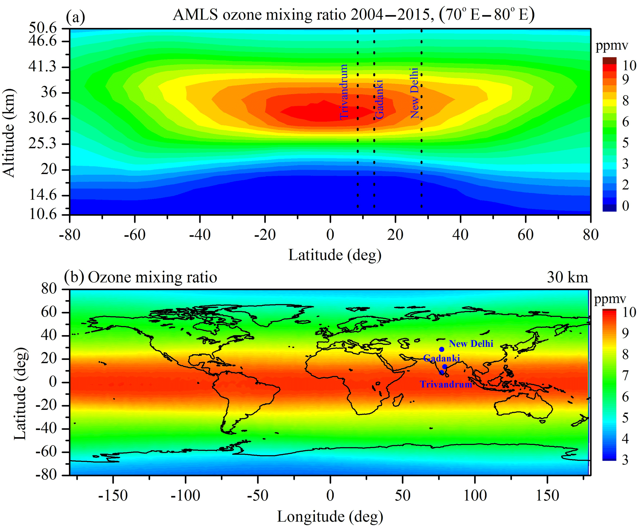
Figure 4 (a) Zonally averaged (70–80^∘ E) ozone mixing ratio over the Indian subcontinent obtained from AMLS during 2004–2015. (b) Time averaged ozone mixing ratio contour at 30 km obtained from AMLS during 2004–2015.

We have calculated systematic error since the standard deviation (SD) between the data sets could not be calculated due to the lack of data points. Usually the systematic error may not be symmetric to the merged data, especially when one of the sources of data is significantly biased compared to the other (Froidevaux et al., 2015). Figure 3a shows the result of systematic error calculation at 21.5 hPa over Trivandrum along with source data. The lower limit of error is determined by HALOE data and the upper limit by SABER data. Systematic error is estimated by calculating the variance via

$$\begin{array}{ll}{\displaystyle }{\mathit{\sigma }}_u^{\mathrm{2}}& {\displaystyle }={\displaystyle \frac{\mathrm{1}}{n_u-\mathrm{1}}}(\sum _k\left(n_{yk}-\mathrm{1}\right){\mathit{\sigma }}_{yk}^{\mathrm{2}}+\sum _k{n}_{yk}{\stackrel{\mathrm{‾}}{Y}}_k^{\mathrm{2}}+n_u{U}_{\mathrm{ref}}^{\mathrm{2}}\\ \text{(4)}& {\displaystyle }& {\displaystyle }-\mathrm{2}{U}_{\text{ref}}\sum _k{n}_{yk}{\stackrel{\mathrm{‾}}{Y}}_k),\end{array}$$

where k represents the given instrument (source), n_yk represents the total number of data from a given source (instrument), ${\mathit{\sigma }}_{yk}^{\mathrm{2}}$ represents the variance of source data, the adjusted time series mean is taken as ${\stackrel{\mathrm{‾}}{Y}}_k$, and $U_{\mathrm{ref}}^{\mathrm{2}}$ is the merged value (which is not necessarily the average value $\stackrel{\mathrm{‾}}{U})$. In this paper we used $U_{\mathrm{ref}}^{\mathrm{2}}=\frac{\mathrm{1}}{n_u}{\sum }_k{n}_{yk}{\stackrel{\mathrm{‾}}{y}}_k$ since we are merging emission-type versus occultation-type instruments. Systematic error is due to bias or drift in the measurement system that affects measurements' accuracy (Latifovic et al., 2012). Figure 3b shows the merged temperature over Trivandrum from 1993 to 2015 after removing the bias.

2.5 Regression analysis

The mean profiles of ozone, temperature, and water vapor are composed of mainly semi-annual oscillation (SAO), annual oscillation (AO) quasi-biennial oscillation (QBO), El Niño–Southern Oscillation (ENSO), and an 11-year solar cycle. It is necessary to remove all these short-term and long-term periodicities in order to estimate the long-term trends. For this purpose we applied regression analysis to the monthly mean profiles of ozone, temperature, and water vapor at each altitude. The general expression of the regression model equation can be written as follows (Randel and Cobb, 1994):

$$\begin{array}{ll}{\displaystyle }T(t,z)& {\displaystyle }=\mathit{\alpha }\left(z\right)+\mathit{\beta }\left(z\right)t+{\mathit{\gamma }}_{\mathrm{1}}\left(z\right){\text{QBO}}_{\mathrm{1}}\left(t\right)+{\mathit{\gamma }}_{\mathrm{2}}\left(z\right){\text{QBO}}_{\mathrm{2}}\left(t\right)\\ \text{(5)}& {\displaystyle }& {\displaystyle }+\mathit{\delta }\left(z\right)\text{Solar}\left(t\right)+\mathit{\epsilon }\left(z\right)\text{ENSO}\left(t\right)+\text{resid}\left(t\right).\end{array}$$

The coefficients, α, β, γ₁, γ₂, δ, and ε are calculated using the following harmonic expression (Kishore et al., 2014):

$$\begin{array}{}\text{(6)}& {\displaystyle }\mathit{\alpha }\left(z\right)=A_o+\sum _{i=\mathrm{1}}^{\mathrm{3}}[A_i\times \cos {\mathit{\omega }}_{i}t+B_i\times \sin {\mathit{\omega }}_{i}t],\end{array}$$

where ${\mathit{\omega }}_i=\mathrm{2}\mathit{\pi }i/\mathrm{12}$.

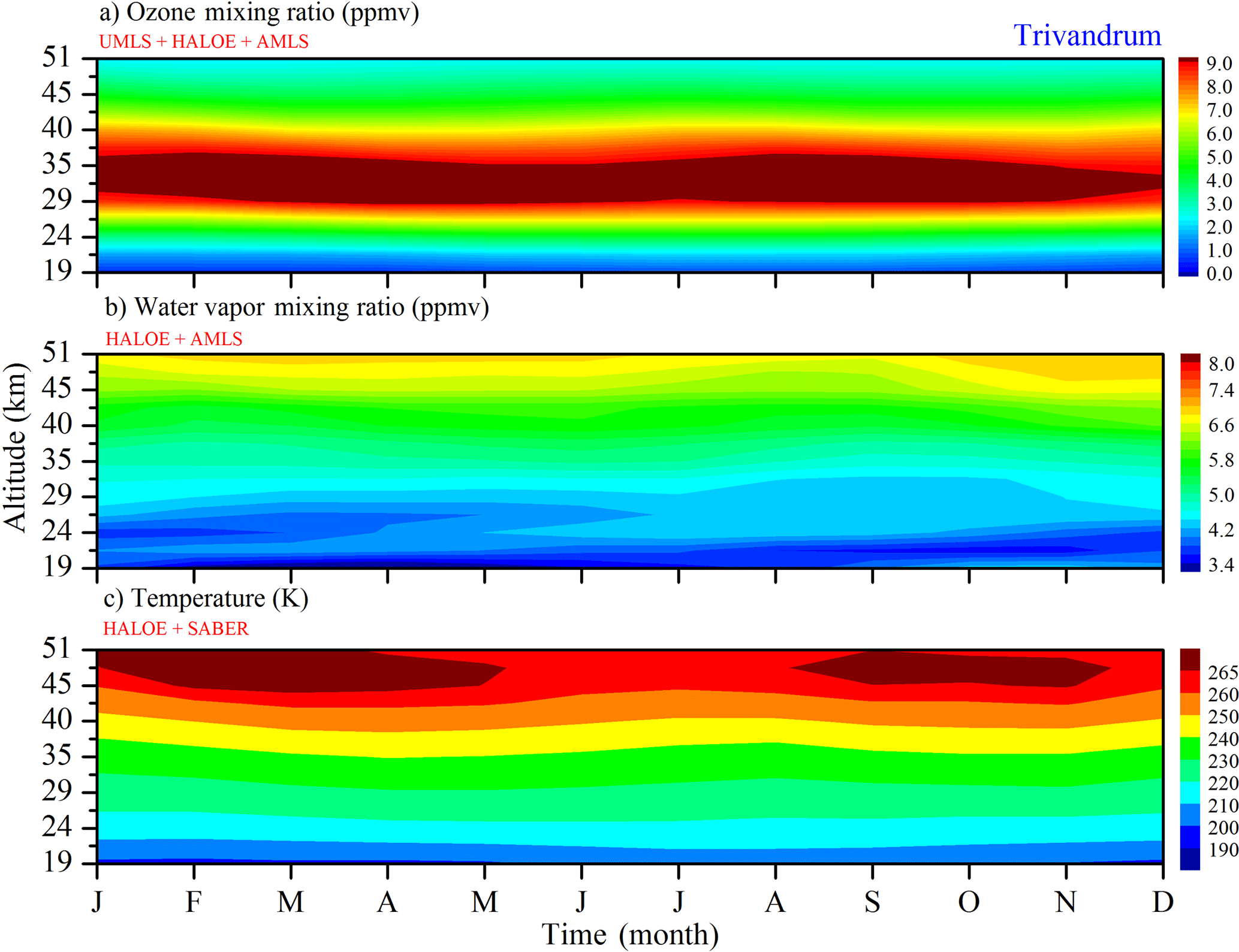
Figure 5 Composite monthly mean contours of bias removed (a) ozone mixing ratio contour constructed using UMLS (1993–199), HALOE (2000–2001), and AMLS (2002–2015), (b) water vapor mixing ratio constructed using HALOE (1993–2004) and AMLS (2005–2015), and (c) temperature constructed using HALOE (1993–2001) and SABER (2002–2015) observations over Trivandrum.

If S is the sum of squares of residuals, N is the length of data, and M is the total number of regression constants (N>M), then the error in the coefficients is given by

$$\begin{array}{}\text{(7)}& \mathit{\sigma }=\sqrt{{\displaystyle \frac{S}{N-M}}(X^{T}X{)}^{-\mathrm{1}}},\end{array}$$

where X is the input data matrix. Singapore (1^∘ N, 104^∘ E) monthly mean QBO zonal wind (m s⁻¹) at 30 hPa is used as a QBO₁ proxy (QBO₁(t)) and QBO zonal wind at 50 hPa is used as a second QBO₂ proxy (QBO₂(t)); these data are available at http://www.geo.fu-berlin.de/met/ag/strat/produkte/qbo. We used Ottawa monthly mean F10.7 cm solar radio flux indices as a proxy (solar(t)) for solar activity. These data may be downloaded from the following website: ftp://ftp.geolab.nrcan.gc.ca/data/solar_flux/monthly_averages/maver.txt. We used the Southern Oscillation Index (SOI), which is calculated from the monthly mean sea level pressure (MSLP) at Tahiti (18^∘ S, 150^∘ W) minus MSLP at Darwin (13^∘ S, 131^∘ E) as a proxy for the El Niño–Southern Oscillation (ENSO(t)). These data are publicly available on the following website: http://www.cpc.ncep.noaa.gov/data/indices/soi.

3 Results and discussion

3.1 Global distribution of ozone: composite mean

While comparing ozone profiles from two different stations, which are separated by ∼ 5^∘ as shown in Fig. 1b, any differences that may arise due to latitudinal variation need to be considered. In order to examine this aspect, in Fig. 4a we plotted the zonal (70–80^∘ E) composite mean of ozone mixing ratio for the period of 2004 to 2015 obtained from AMLS. The dotted lines in the figure mark the locations of Trivandrum, Gadanki, and New Delhi. The ozone concentrations at the ozone peak altitude of Trivandrum and Gadanki are nearly the same, which means that the difference which we observed in Fig. 1b is not due to the difference in latitudes of the two stations but can be the combined result of change in chemistry and dynamics. We have checked the same with ozone number density. Figure 4b shows the mean ozone mixing ratio distribution over the globe at 30 km (ozone peak altitude at Trivandrum and Gadanki). Trivandrum, Gadanki, and New Delhi were represented in the figure as blue dots. From this figure it is clear that the ozone mixing ratio over Trivandrum and Gadanki at 30 km is higher than that of New Delhi at 30 km. There must be no significant difference between Trivandrum and Gadanki ozone mixing ratio in the stratosphere but we can expect a difference between Trivandrum and New Delhi. Hence it will be interesting to investigate the regional differences in ozone distribution over the Indian subcontinent.

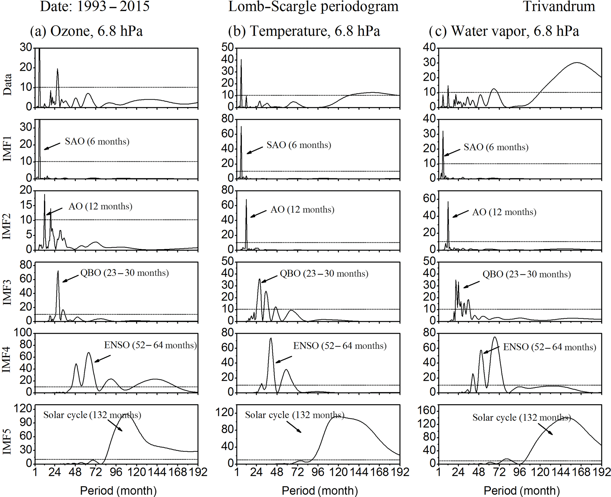
Figure 6 LS periodograms obtained from various IMFs for (a) ozone, (b) temperature, and (c) water vapor over Trivandrum at 6.8 hPa. The dotted line shows the 99 % confidence level.

3.2 Climatology of ozone, water vapor, and temperature

Figure 5a, b, and c show the climatology of the monthly mean ozone mixing ratio (OMR), water vapor mixing ratio, and temperature, respectively, over Trivandrum in the 20 to 50 km attitude range, calculated from merged data sets. An OMR maximum is observed between 30 and 37 km. For the same time period we calculated water vapor mixing ratio using UARS HALOE and AMLS observations. In the lower stratosphere (∼ 20–23 km), an enhancement of water vapor is found during the wintertime, and later it started to decrease. Initially the decreasing of water vapor with altitude is observed; however, water vapor concentration increases with altitude above the middle stratosphere. Water vapor shows a SAO in the upper stratosphere, with a maximum in pre-monsoon and post-monsoon periods, whereas in the lower stratosphere it shows more of an AO, with a maximum during the summer. Temperature shows an SAO, with a peak occurring in pre-monsoon and post-monsoon periods, which is more prominently seen in the upper stratosphere than the lower stratosphere. Heating in the upper stratosphere is observed over Trivandrum during January–April and September–November, which is seen in Fig. 5c.

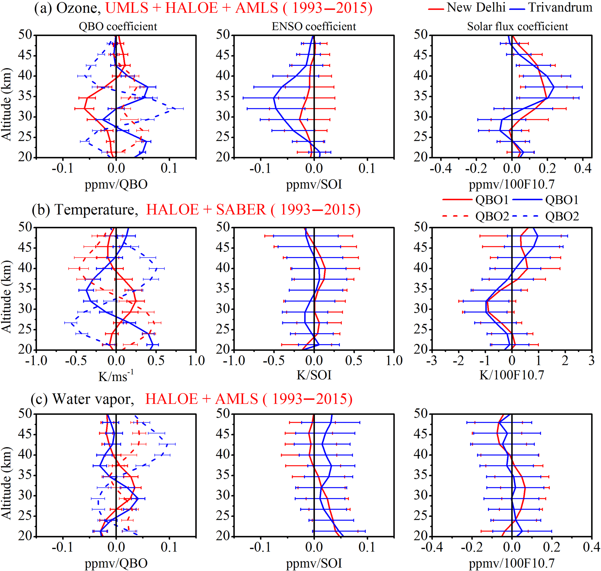
Figure 7 Altitude profile of the response of the (a) ozone mixing ratio obtained using combined measurements of UMLS, HALOE, and AMLS, (b) temperature from HALOE and SABER, and (c) water vapor mixing ratio from HALOE and AMLS over Trivandrum (blue) and New Delhi (red) to the QBO, ENSO, and the solar cycle. The solid line represents 30 hPa QBO wind (QBO₁) and the dashed line represents 50 hPa QBO wind (QBO₂).

3.3 Intrinsic mode function (IMF) analysis

Before proceeding to the regression analysis to investigate the long-term trends in ozone, temperature, and water vapor, we examined the data for the presence of any dominant periodicities. For this analysis, we used the empirical mode decomposition (EMD) method. This method is in contrast to the other methods and works in the temporal domain directly rather than in the corresponding frequency domain (Huang and Wu, 2008). The EMD method breaks down the nonlinear oscillation patterns naturally into a number of characteristic intrinsic mode function (IMF) components (Zhen-Shan and Xian, 2007). This technique is derived from the simple assumption that the IMF is a function that satisfies the following two conditions. (1) In the whole data set, the number of extreme points and the number of zero crossings are either equal or differ at most by 1. (2) At any point, the mean value of the envelopes defined by local maxima and local minima is zero (Huang et al., 1998). Once the extrema are identified, we connect the maxima and minima by using cubic spline interpolation to form upper and lower envelopes. Their mean (m1) is subtracted from the original data (x(t)), which can be represented as h₁. However, h₁ is still not a stationary oscillation pattern. Hence we replaced the original data with h₁ and repeated the process and calculated h₂. This process is repeated until the mean value of the envelope becomes zero or close to zero, with the SD < 0.2. Through this process we get the first IMF component, c₁. We removed the first IMF component from the original time series as follows.

$$\begin{array}{}\text{(8)}& {\displaystyle }{r}_{\mathrm{1}}=x\left(t\right)-c_{\mathrm{1}}\end{array}$$

Since r₁ still contains information about the long periods, we repeated the entire process by replacing r₁ with the original data.

$$\begin{array}{}\text{(9)}& {\displaystyle }{r}_{\mathrm{2}}=r_{\mathrm{1}}-c_{\mathrm{2}}\end{array}$$

The above process is repeated n times, and all the possible IMFs and the residue are calculated. The original time series can be represented as

$$\begin{array}{}\text{(10)}& x\left(t\right)=\sum _{i=\mathrm{1}}^n{c}_i+r_n,\end{array}$$

where c_i is the possible IMF and r_n is the residue.

The monthly ozone mixing ratio perturbation was broken down into seven IMFs using the EMD method, and the amplitude spectrum of the ozone mixing ratio perturbation is calculated using Lomb–Scargle (LS) analysis and is shown in Fig. 6a. The same analysis is carried out for the temperature and water vapor mixing ratio and is shown in Fig. 6b and c, respectively. In the figure we have shown the analysis at 6.8 hPa for ozone, temperature, and water vapor. In each periodogram, the dashed line indicates the 99 % confidence level. From this figure it is clear that the dominant peaks are located near the SAO, AO, QBO, ENSO, and the solar cycle. The uppermost panel in the Fig. 6 is the Lomb–Scargle periodogram of original data. The first and second IMFs represent the SAO and AO (from top). The QBO period shown in the third IMF ranges from 23 to 30 months. The fourth IMF shows the ENSO periods, which range from 52 to 64 months. The solar cycle is shown in the fifth IMF, which has a period of approximately 11 years (132 months). The solar cycle spectrum is broader and ranges from a 10-year to a 12-year period.

3.4 Long-term trends

The LS periodogram analysis presented in the previous section revealed the presence of dominant periodicities in stratospheric ozone, temperature, and water vapor. In some years monthly averaged data points are missing in the middle of the time series. Since the trend analysis is strongly dependent on the points near the beginning and end of the data sets, midpoints do not contribute much (Saraf and Beig, 2004). With this confidence we proceeded with linear trend analysis.

3.4.1 Ozone, temperature, and water vapor response to the QBO, ENSO, and solar cycle

Figure 7a shows the ozone response to the QBO, ENSO, and 11-year solar cycle derived from the 23 years of merged satellite observations for both Trivandrum and New Delhi along with SD. We have used two orthogonal QBO wind (30 and 50 hPa) components for the present study. The solid line in Fig. 7a shows the ozone response to 30 hPa QBO wind (QBO₁) and the dashed line shows 50 hPa QBO wind (QBO₂). The ozone responses to QBO over Trivandrum and New Delhi are quite different. The QBO₁ response over Trivandrum shows a double peak structure in the lower and middle stratosphere, with a maximum response around 24 km (0.056 ± 0.016 ppmv/QBO) and a minimum around 30 km (−0.025 ± 0.025 ppmv/QBO). Ozone response to QBO₁ over New Delhi is negative in the lower stratosphere and maximum is around 32 km (−0.059 ± 0.036 ppmv/QBO). The ozone response to the QBO₁ and QBO₂ (dashed line) are quite opposite because the QBO₃₀ and QBO₅₀ are predominantly out of phase. The ozone response to ENSO is larger over Trivandrum than New Delhi. The ENSO response is negative over both of the stations. The ENSO effect on ozone in the lower and upper stratosphere is negligible when comparing over New Delhi and Trivandrum. The ozone response to the solar cycle is positive in the lower stratosphere over both of the stations. However this decreases with increasing altitude and becomes negative above 25 km. The solar flux coefficient shows similar characteristics over both the stations, with a positive peak around 35–40 km. The larger response of solar cycle is found in the middle stratosphere over both stations, with peaks around 37 km (0.23 ± 0.15 ppmv/100 sfu) and 35 km (0.19 ± 0.15 ppmv/sfu) over Trivandrum and New Delhi, respectively.

Figure 7b shows the temperature response to QBO, ENSO, and the 11-year solar cycle derived from the multi-satellite observations. The temperature response to the QBO₁ and QBO₂ over Trivandrum and New Delhi shows an opposite structure. The QBO₁ response to temperature over Trivandrum is larger in the lower and middle stratosphere. A positive response is found in the lower and upper stratosphere, whereas a negative response is higher in the middle stratosphere. The QBO₁ effect on ozone over New Delhi is larger near the middle stratosphere, and a positive maximum is found around 32 km (0.24 ± 0.22 K/QBO). The temperature response to QBO₂ over Trivandrum and New Delhi shows a mirror image kind of structure. The ozone response to QBO₂ is larger than to QBO₁. The temperature response to ENSO over Trivandrum and New Delhi is found to be similar in the middle and upper stratosphere. The effect of ENSO on Trivandrum temperature is negative up to 32 km. New Delhi shows an opposite result, being negative below 24 km and becoming positive through the middle stratosphere to the upper stratosphere. The temperature response to ENSO over Trivandrum and New Delhi shows similar characteristics above the middle stratosphere. The temperature response to the solar cycle is negative or low in the lower stratosphere, and its magnitude increases with altitude and attains a maximum value of 0.97 ± 79 and 0.92 ± 1.0 K/100 F10.7 over Trivandrum and New Delhi, respectively, around 30 to 32 km. Further, with increasing altitude, the magnitude of solar response decreased and it became positive over both the stations beyond 38 km.

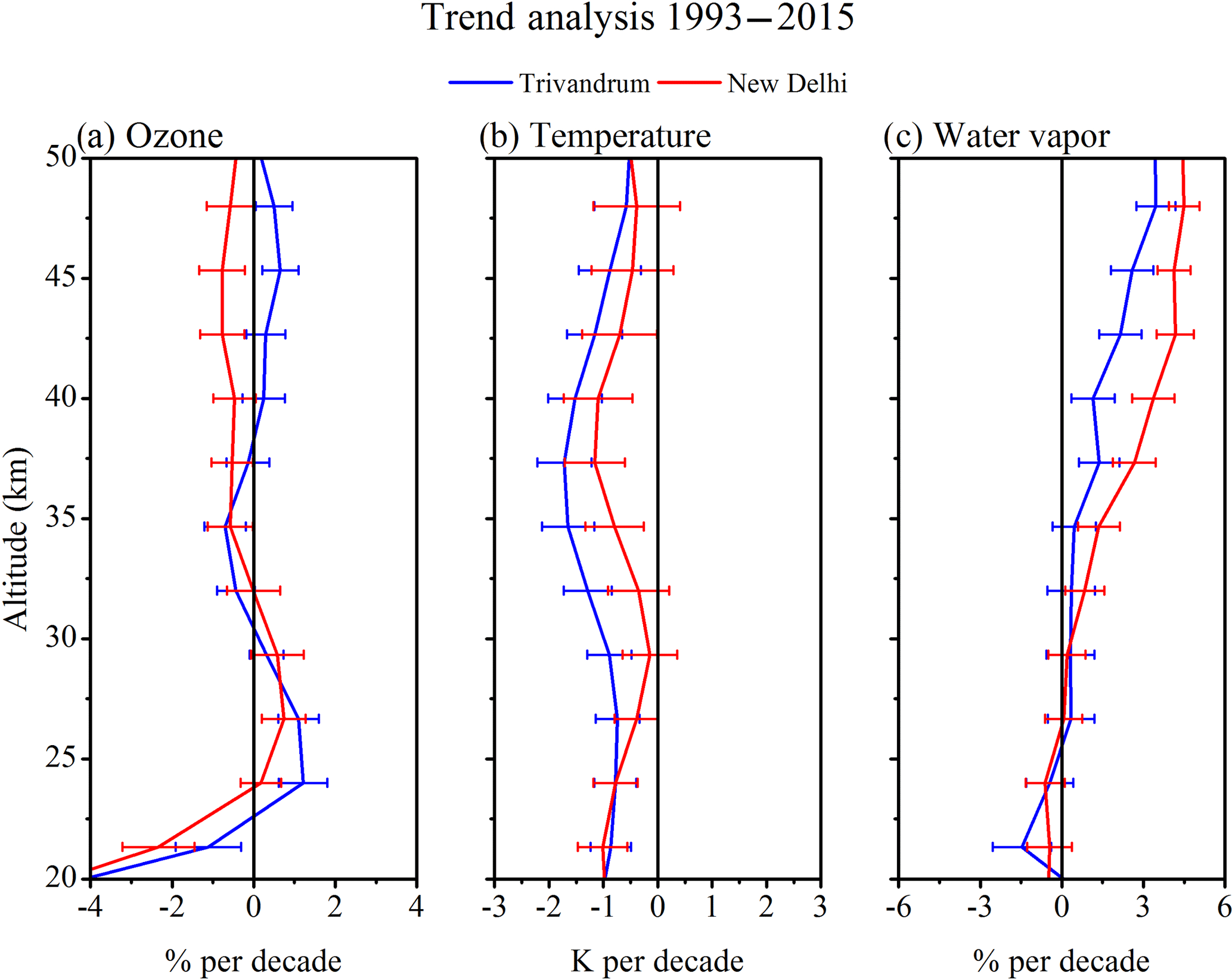
Figure 8 Vertical variation of trend observed in the (a) ozone mixing ratio (in % decade⁻¹), (b) temperature (in K decade⁻¹), and (c) water vapor mixing ratio (in % decade⁻¹) obtained from multi-satellite observations over Trivandrum (blue) and New Delhi (red) during 1993–2015.

Figure 7c shows the water vapor response to QBO, ENSO, and the solar cycle over Trivandrum and New Delhi. The water vapor response to QBO₁ over Trivandrum and New Delhi is negative in the lower and upper stratosphere. It shows a positive peak in the middle stratosphere, with a maximum 0.04 ± 0.02 and 0.03 ± 0.02 ppmv/QBO around 30 and 32 km over Trivandrum and New Delhi, respectively. The ENSO coefficient of water vapor shows similar characteristics over Trivandrum and New Delhi in the lower stratosphere. The water vapor response to the ENSO becomes negative in the upper stratosphere of New Delhi, but not over Trivandrum. The solar flux coefficient over Trivandrum is positive in the lower stratosphere and it becomes negative in the middle and upper stratosphere. In the case of New Delhi, the water vapor response to the solar flux is different from Trivandrum. It shows a positive peak in the middle stratosphere, and the magnitude decreased with altitude and became negative in the upper stratosphere. The larger SD in the ENSO and solar cycle coefficients in Fig. 7 may be due to the larger variability of ENSO (52–60 months) and the solar cycle (10–12 years) than QBO (23–30 months).

3.4.2 Long-term trends in ozone, temperature, and water vapor

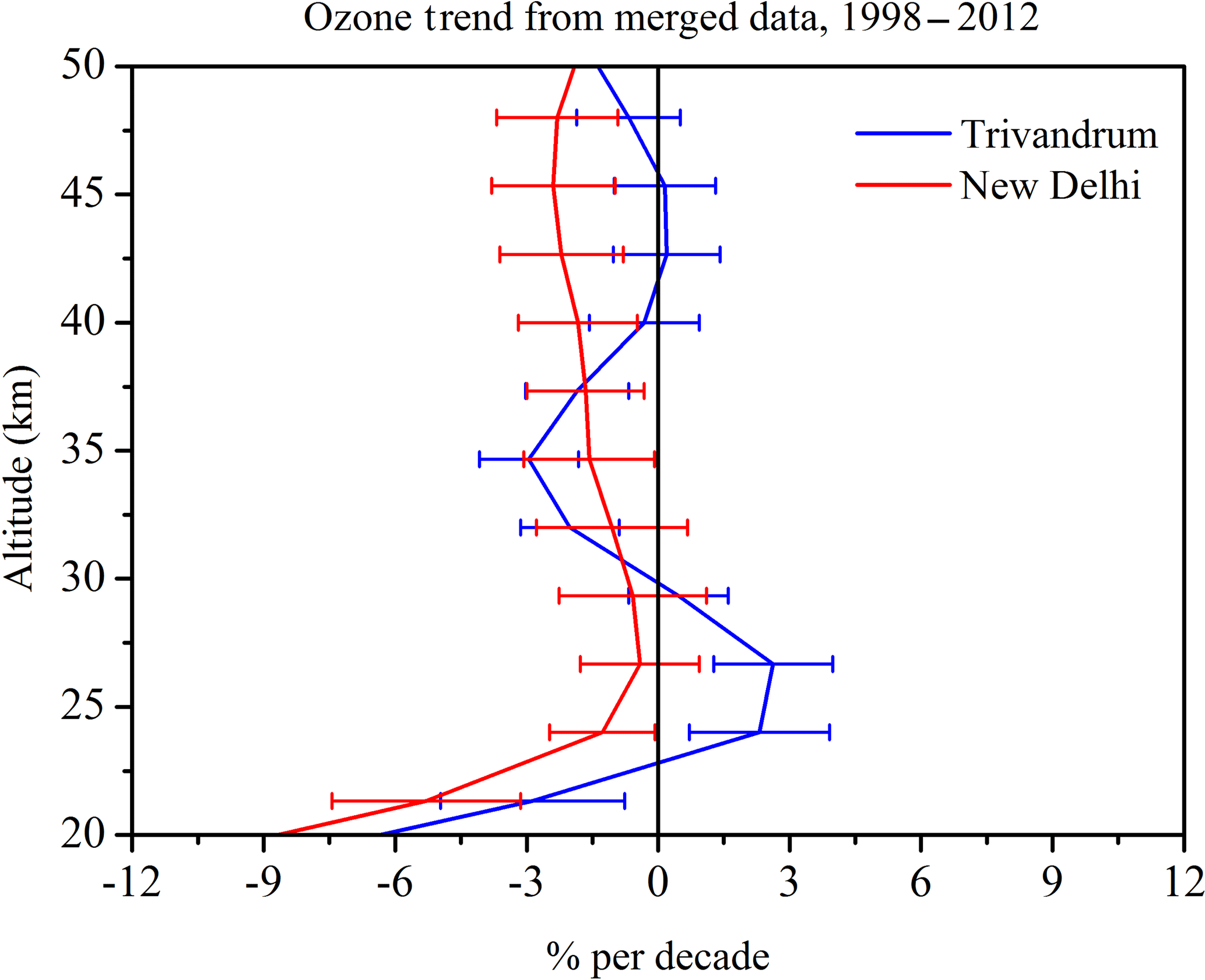
Figure 8a shows the altitude profile of ozone trends per decade (in percentage) with 2 SD obtained over Trivandrum and New Delhi during 1993 to 2015. Ozone shows a significant decreasing trend in the lower stratosphere over both stations. The decreasing trend is higher in the lower stratosphere, and its magnitude decreases with altitude. Sioris et al. (2014) also reported a significant decreasing trend in ozone in the lower stratosphere (18.5–24.5 km) during 1984 to 2012 from merged satellite data of SAGE II and OSIRIS over a latitude bin 7.5^∘ N–7.5^∘ S. In our analysis the ozone trend becomes positive over Trivandrum and New Delhi between 22.5 and 30 km, and the positive trend is higher over Trivandrum than New Delhi. The positive trend in ozone is significant over Trivandrum and it is only significant around 27 km over New Delhi. The trend reverses to negative around 30 km over both the stations, and it remains negative over New Delhi. The upper stratospheric ozone trend over Trivandrum is positive and it is significant in the higher altitudes. In general, the decreasing trend in ozone in the middle and upper stratosphere over New Delhi is statistically significant. Similarly, the decreasing trend in ozone over Trivandrum is also significant around 35 km. The statistically significant positive trend in the upper stratospheric ozone over Trivandrum is the major difference we found between Trivandrum and New Delhi. The trend reported by Harris et al. (2015) using revised multiple data sets shows similar results over the tropics (20^∘ N–20^∘ S) during 1998–2012 (their Fig. 6). To compare the trend with these results, we have estimated the ozone trend over Trivandrum and New Delhi during 1998–2012, shown by Fig. A1 in Appendix A. We found a good agreement with the ozone trend from Harris et al. (2015), estimated using GOZCARDS data (their Fig. 6) over the tropics. A maximum increasing trend (2.62 ± 1.35 % decade⁻¹) is observed around 27 km, and a maximum decreasing trend (−2.94 ± 1.13 % decade⁻¹) in ozone is found around 35 km. The decreasing trend in ozone over the tropics in the middle stratosphere also exactly matches with the reported observations during this period. The increasing and decreasing ozone trends over Trivandrum are statically significant during this time period. In the case of New Delhi, an extratropical station, in general, statistically significant decreasing trend in the stratospheric ozone is found. Gebhardt et al. (2014) also observed a positive trend between 20 and 30 km and a negative trend between altitudes of 30 and 40 km using SCIAMACHY limb measurement for the time period 2002–2012 for the zonal mean in the complete tropical latitudes (20^∘ N–20^∘ S). The current analysis shows that there is an increase in the ozone concentration around 23–30 km; this is consistent with that observed in Fig. 1b. Ozone trend estimation by varying the period is also carried out over both the stations, which is shown by Fig. A2 in Appendix A. The lower stratospheric (above 24 km) increasing trend in ozone over both stations is consistent, and similarly, the decreasing ozone trend below 24 km is also found to be consistent over Trivandrum than New Delhi. The trend estimation from 2000, 2001, and 2002 to 2015 over New Delhi shows an increasing trend in ozone from ∼ 21 km upwards. A middle stratospheric ozone decreasing trend over the tropics is also found during all these periods. The major difference between Trivandrum and New Delhi is in the upper stratospheric ozone trend. An increasing trend in upper stratospheric ozone is found during these years over Trivandrum, and a decreasing trend is found over New Delhi.

Figure 8b shows the temperature trend over Trivandrum and New Delhi during 1993–2015. UARS HALOE and SABER data are merged together to make a 23-year time series. Though the two stations are separated by ∼ 20^∘, we observed similar features in the temperature trend. The trend is almost identical below 25 km; above that the cooling trend is higher over Trivandrum than New Delhi. The maximum cooling trend is observed in the middle stratosphere around 35 to 40 km over both stations. The cooling trend is maximum around 37 km over Trivandrum (1.71 ± 0.49 K decade⁻¹) and New Delhi (1.15 ± 0.55 K decade⁻¹). These results are consistent with the recent results reported by Kishore et al. (2014) using Gadanki lidar data (for the period 1998–2011), where they found strong cooling near 38 km (∼ 1.83 ± 1.1 K decade⁻¹) and 56 km (∼ 2 K decade⁻¹). The simultaneous satellite trend analysis over Gadanki showed a cooling trend near stratopause (50 km) altitude, which we have seen over Trivandrum and New Delhi. The cooling trend is statistically significant in all the altitudes over Trivandrum. In the case of New Delhi, the cooling trend is not significant in the upper stratosphere and is around 30 km in the middle stratosphere.

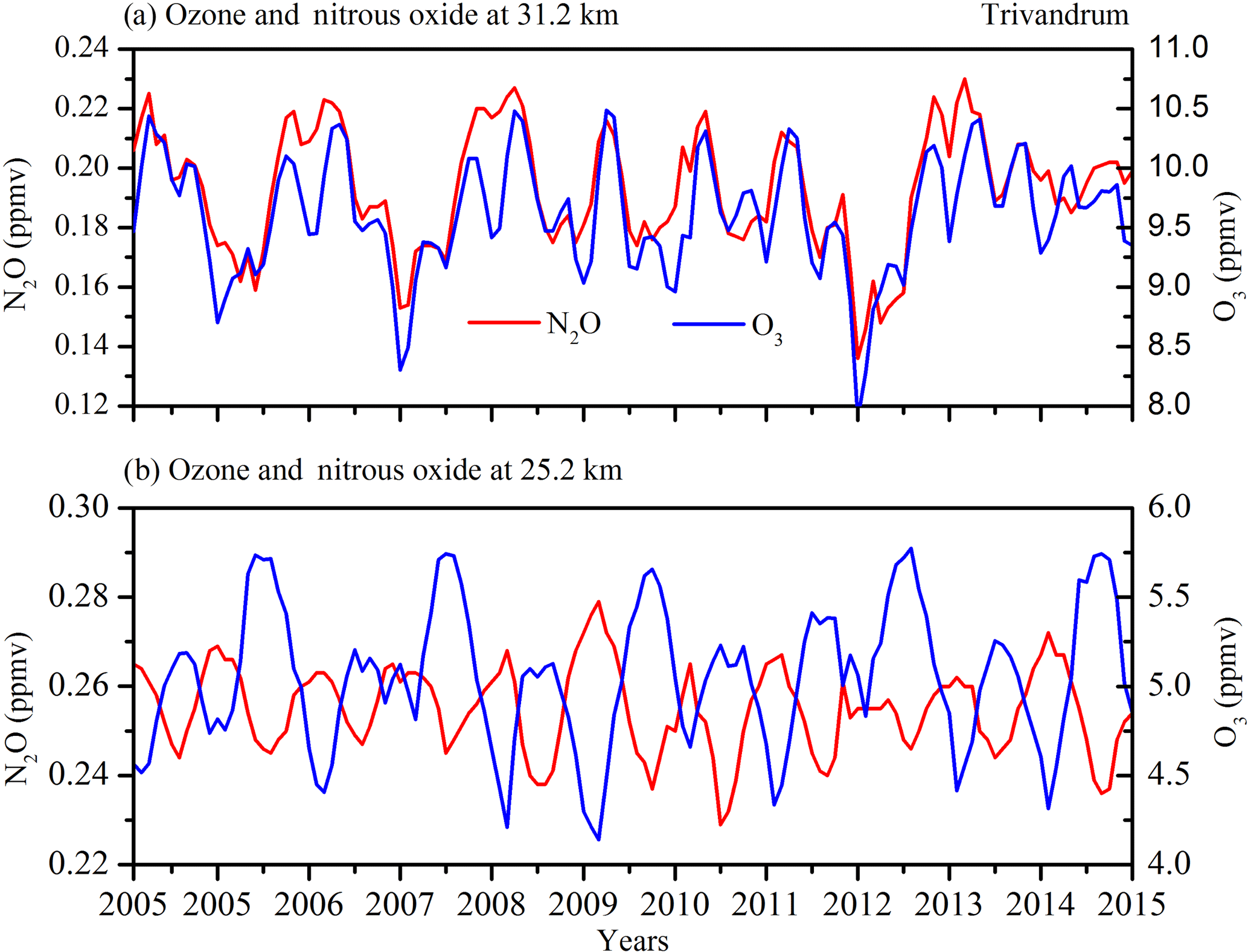
Figure 9 Monthly averaged N₂O (red) and O₃ ratios at (a) 31.2 km and (b) 25.2 km over Trivandrum obtained from AMLS measurements.

Water vapor trends in the stratosphere are shown in Fig. 8c. UARS HALOE and AMLS observations are used to obtain 23 years of time series in the stratosphere from 1993 to 2015. Water vapor shows a non-significant decreasing trend in the lower stratosphere over Trivandrum and New Delhi. The increasing trend is found above 24 km over both the stations; however, the trend is only significant in the upper stratosphere. In the upper and middle stratosphere, the water vapor trend is higher over New Delhi.

We now discuss the observed trend in ozone in the light of the trends in temperature and water vapor. It is reported that tropospheric ozone shows, in general, an increasing long-term trend due to anthropogenic sources (IPCC, 2013). A decrease in ozone concentration is expected to result in a decrease in temperature and vice versa as ozone is the major heat source in the stratosphere. The observed trends in ozone and temperature, in general, are in accordance with this. It may be noted that temperature has a negative feedback effect on ozone due to temperature dependence of chemical reaction rates of ozone. Thus, the direct relations between ozone and temperature will be tempered by this negative feedback between the two. Ozone above 10 hPa is mostly under the control of photochemical processes, and below this altitude, both the transport and chemistry control the ozone concentration (Butchart, 2014). Hence, the transport effect is at a maximum in the lower stratosphere and the temperature effect is at a maximum in the upper and middle stratosphere. Previous studies on stratospheric ozone have shown tropical upwelling to be the major reason for the reduction in lower tropical stratospheric ozone (Oman et al., 2010). Therefore, the decreasing ozone trend in the lower stratosphere is mainly due to the strengthening of the Brewer–Dobson Circulation (BDC). Rosenfield et al. (2002) attributed the reduction in the tropical lower stratospheric ozone to the combined effect of increased upwelling and the decreased production of ozone to the “reverse self-healing”, i.e., the reduction in the production of lower stratospheric ozone as a result of increasing upper and middle stratospheric ozone, which thereby causes less ultraviolet radiation to penetrate to the lower stratosphere. The decreasing ozone concentration may be the prime reason for the cooling of the lower stratosphere over the tropics.

Here the question is regarding the cause for the observed positive ozone trends around 23 to 30 km over Trivandrum and New Delhi. It is known that the catalytic reactions involving ClO_x, NO_y, and HO_x play a major role in the destruction of ozone in the stratosphere. These are mainly of anthropogenic origin in the troposphere. ClO_x can be effective in the ozone destruction in the lower stratosphere. NO_y and HO_x can be effective in the upper stratosphere (> 30 km). The observed negative trends in ozone in the altitudes above 30 km can be attributed to an expected positive trend in NO_y and HO_x due to anthropogenic sources. The observed positive trend in water vapor, which yields HO_x on photo dissociation, is consistent with this conclusion. The reduction in the decreasing trend in ozone in the lower stratosphere (25–30 km) can be caused by a reduction in ClO_x. Note that ClO_x is also of anthropogenic origin, and its reduction is reported over the tropics (Connor et al., 2013; Jones et al., 2011). Actions taken under the Montreal Protocol have led to a decrease in ozone-depleting substances (ODSs). Equivalent effective stratospheric chlorine has declined to 10–15 % from the peak value in the last 10 to 15 years (WMO, 2014). The atmospheric abundance of ODSs will continue to decrease in the coming decades; however, the increase in N₂O will become the primary source of nitrogen oxides in the stratosphere and will become more important in future ozone depletion (WMO, 2014). The increasing trend in the tropical upper stratospheric ozone is attributed to the slowing down of chemical loss cycles due to the cooling of the stratosphere (Rosenfield et al., 2002). The cooling of the stratosphere has direct and indirect effects on ozone loss. The direct effect is that it will slow down the ozone recombination reaction O + O₃ → 2 O₂. The indirect effect of stratospheric cooling is the decrease in production of NO_y per N₂O molecules and the increase of the loss rate of NO_y (Rosenfield and Douglass, 1998).

3.5 Chemistry of nitrous oxide

As mentioned earlier, the tropical mid-stratosphere ozone is more sensitive to NO_y (NO + NO₂) changes. Photo-chemical reactions of N₂O are the main source of NO_y in the tropical mid-stratosphere. The concentration of N₂O decreases with the photo-dissociation and produces NO_y, and this will undergo catalytic ozone destruction at these altitudes. The dissociation of N₂O is connected with a coupled chemical–dynamical effect. The observed trend is also strongly dependent on the vertical transport rate. At altitudes at which the transport is slow, more N₂O will dissociate and form NO_y. Nedoluha et al. (2015), using HALOE observations during 1992 to 2005, reported that the NO + NO₂ is generally increasing, and this increase showed the ozone loss to be ∼ 10 hPa over the tropics.

Monthly mean AMLS O₃ and N₂O are presented in Fig. 9 from 2005 to 2015 at two different altitudes, 31.2 and 25.2 km over Trivandrum, to show the altitude-dependent chemistry of O₃, N₂O, and NO. A strong positive correlation (R=0.83) between O₃ and N₂O is clearly visible in the middle stratosphere (at altitude 31.2 km), and at 25.2 km we observed a well pronounced negative correlation ($R=-\mathrm{0.73}$) between O₃ and N₂O. Nedoluha et al. (2015) also observed a similar positive correlation between O₃ and N₂O at 10 hPa between 5^∘ S and 5^∘ N. The N₂O loss and production of NO_y reactions can be found in Brasseur and Solomon (2005) and Olsen et al. (2001).

The photolysis of N₂O is not strong below 10 hPa (∼ below 30 km), odd nitrogen loss by reactions is higher, and the rapid increase of O(¹D) concentration above the middle stratosphere (∼ 40 km) (Brasseur and Solomon, 2005) limited the ozone loss by odd nitrogen compounds to the middle stratosphere. However, correlation or anti-correlation between N₂O and O₃ does not necessarily provide evidence for a chemical control of NO_y on O₃, as in particular in the lower stratosphere, transport will have a strong effect on both N₂O and O₃. Nitrous oxide concentration decrease over the equator and the tropics is less rapid compared to higher latitudes. This is probably because of the rate of transport associated with the rising branch of the BDC at these latitudes. Hence, a much higher concentration of N₂O is reaching the tropical and equatorial middle and upper stratosphere, as does the photo-dissociation of N₂O by reacting with odd oxygen (O(¹D)).

4 Summary and conclusions

Using multi-satellite observations, we constructed merged ozone, temperature, and water vapor data during the time period 1993–2015. Using these merged data products, covering more than 2 decades, long-term trends in ozone, water vapor, and temperature over the Indian region are investigated. The contributions of various long-period oscillations to the observed trends like SAO, AO, QBO, ENSO, and the solar cycle in the stratosphere over Trivandrum and New Delhi are also investigated. The main conclusions drawn from the current study are summarized in the following.

Ozone shows a significant decreasing trend in the lower stratosphere (20 to 24 km) during 1993–2015. The strengthening of the BDC is the major cause for this decreasing ozone trend in the tropical lower stratosphere. The trend becomes positive above 24 km over Trivandrum and New Delhi. The decreasing trend is around 5 % decade⁻¹ around 20 km over both the stations.

A decreasing trend in ozone is observed in the middle stratosphere over both the stations. The decreasing trend is higher over Trivandrum when compared to that observed over New Delhi. The negative trend in the ozone over Trivandrum reaches a maximum of 0.69 ± 0.50 % decade⁻¹ around 34 km. This decreasing trend in ozone is mainly due to the odd nitrogen reactions. However, the production of NO_y from N₂O decreases as an indirect effect of stratospheric cooling.

Temperature shows a cooling trend with a maximum around 37 km over Trivandrum (1.71 ± 0.49 K decade⁻¹) and New Delhi (1.15 ± 0.55 K decade⁻¹). These results are consistent with those reported using Gadanki lidar observations. Lower stratospheric cooling is the result of a reduction in ozone due to the strengthening of tropical upwelling.

The water vapor trend is positive in the middle and upper stratosphere over both the stations; this may be due to the increase in methane concentration in the stratosphere.

The QBO response to ozone shows more regional dependence than that of water vapor and temperature. The solar response of the ozone and temperature over both stations shows similar features in the stratosphere except at higher altitudes (40–50 km).

The current study on stratospheric ozone trends shows that ozone concentration is decreasing in the middle and lower stratosphere at a statistically significant rate. The trend analysis is highly dependent on the starting and ending years. This has been shown in Figs. A1 and A2. The maximum ozone decreasing trend in the middle stratosphere is found during 1998–2012 over the tropics. This is consistent with earlier results. The middle and lower stratospheric ozone loss will be an important issue over the tropics in the future along with the increasing trend in the upper tropospheric ozone. This reduction in lower stratospheric ozone by transport will increase the ultraviolet index over the tropics. The effect of the QBO on ozone, temperature, and water vapor has to be investigated in the future. The subtropical barrier plays an important role in the horizontal mixing of trace gases between the tropical and subtropical stratosphere. Detailed analyses of trace gases' distribution and the modulation of the subtropical barrier by QBO are required to understand the role of the subtropical barrier in the observed trend.

Appendix A

Figure A1 Ozone trend (% decade⁻¹) estimated over Trivandrum (blue) and New Delhi (red) during 1998–2015.

Figure A2 Ozone trend (% decade⁻¹) estimated over Trivandrum and New Delhi during different time periods.