Magnetosphere dynamics during the 14 November 2012 storm inferred from TWINS, AMPERE, Van Allen Probes, and BATS-R-US–CRCM

During the 14 November 2012 geomagnetic storm, the Van Allen Probes spacecraft observed a number of sharp decreases (“dropouts”) in particle fluxes for ions and electrons of different energies. In this paper, we investigate the global magnetosphere dynamics and magnetosphere–ionosphere (M–I) coupling during the dropout events using multipoint measurements by Van Allen Probes, TWINS, and AMPERE together with the output of the two-way coupled global BATS-R-US–CRCM model. We find different behavior for two pairs of dropouts. For one pair, the same pattern was repeated: (1) weak nightside Region 1 and 2 Birkeland currents before and during the dropout; (2) intensification of Region 2 currents after the dropout; and (3) a particle injection detected by TWINS after the dropout. The model predicted similar behavior of Birkeland currents. TWINS low-altitude emissions demonstrated high variability during these intervals, indicating high geomagnetic activity in the near-Earth tail region. For the second pair of dropouts, the structure of both Birkeland currents and ENA emissions was relatively stable. The model also showed quasi-stationary behavior of Birkeland currents and simulated ENA emissions with gradual ring current buildup. We confirm that the first pair of dropouts was caused by large-scale motions of the OCB (open–closed boundary) during substorm activity. We show the new result that this OCB motion was associated with global changes in Birkeland (M–I coupling) currents and strong modulation of low-altitude ion precipitation. The second pair of dropouts is the result of smaller OCB disturbances not related to magnetospheric substorms. The local observations of the first pair of dropouts result from a global magnetospheric reconfiguration, which is manifested by ion injections and enhanced ion precipitation detected by TWINS and changes in the structure of Birkeland currents detected by AMPERE. This study demonstrates that multipoint measurements along with the global model results enable the reconstruction of a more complete system-level picture of the dropout events and provides insight into M–I coupling aspects that have not previously been investigated.

Keywords. Magnetospheric physics (magnetosphere–ionosphere interactions; magnetospheric configuration and dynamics); space plasma physics (numerical simulation studies)

1 Introduction

Lobe encounters and associated particle dropouts are considered to be an important indicator of magnetospheric reconfiguration during active times (Sauvaud and Winckler, 1980; Moldwin et al., 1995; Kopanyi and Korth, 1995). The particle dropouts during lobe excursions are distinguished by very low particle fluxes for both ions and electrons starting from a few hundred eV. Analysis of data from geosynchronous spacecraft (Thomsen et al., 1994; McComas et al., 1994; Moldwin et al., 1995, 1998) has determined the properties of lobe encounters and their dependence on season and IMF orientation. Moldwin et al. (1995) found that all lobe encounters observed at geosynchronous orbit can be divided into two broad groups: near-midnight lobe encounters and flank lobe encounters. The near-midnight lobe encounters were mostly associated with the substorm activity, whereas the flank lobe encounters were related to drastic reconfigurations of the magnetosphere during significant variations in solar wind parameters. Kopanyi and Korth (1995) found that some cases of particle dropouts and lobe encounters in the morning sector were also related to substorm activity.

Particle dropouts during lobe encounters are distinguished from more energetic particle dropouts both observationally and physically. Flux decreases in the 10 keV to MeV range, with no substantial dropout for the low-energy population, are observed more frequently and have different statistical properties than lobe excursions (Thomsen et al., 1994). These energetic particle dropouts are caused not by crossings of the lobe boundary but rather by the adiabatic dynamics of trapped particles during geomagnetic storms and substorms, the so-called Dst effect (Dessler and Karplus, 1961; Li et al., 1997).

Two recent papers reported observations of particle dropouts by Van Allen Probes and other spacecraft for the 14 November 2012 geomagnetic storm (Hwang et al., 2015; Dixon et al., 2015). This storm was a moderate event with minimum Dst of −108 nT at 08:00 UT on 14 November and a recovery phase extending to 16 November. During 02:00–05:00 UT of 14 November, both Van Allen Probes A and B detected several sharp decreases in particle flux, i.e., order-of-magnitude drops that occurred suddenly (onsets within a few minutes) followed by sustained, reduced flux levels lasting up to ∼ 10 min. Dropouts occurred for both ions and electrons across an extremely broad (eV to MeV) energy range. The dropouts were observed in the dawn sector, 04:00 to 06:00 MLT, at radial distances of 4.6 to 5.8 R_E near the GSM equator (Z_GSM ≈ −1.8 to −0.5 R_E) and contained lobe plasma (Dixon et al., 2015). This storm is of particular interest since multipoint measurements from Van Allen Probes, geostationary satellites, TWINS, Geotail, THEMIS, and AMPERE were available, making possible the reconstruction of a global picture of magnetospheric dynamics during the event.

There are two hypotheses for the cause of the 14 November dropouts. Hwang et al. (2015), hereinafter referred to as Hw15, analyzed the event using data from Van Allen Probes, geostationary satellites, and THEMIS. They found that the dropouts were observed by geostationary satellites across a broad MLT range in the dusk, midnight, and morning sectors. Hw15 suggested that the dropouts were observed when the magnetic flux ropes from the tail moved through the spacecraft location. According to this interpretation, these flux ropes were formed along the reconnection X line in the near-Earth plasma sheet.

An alternate interpretation by Dixon et al. (2015), hereinafter called Di15, suggested that the dropouts on 14 November 2012 were caused by crossing the boundary between open and closed magnetic field lines (the open–closed boundary or OCB) and lobe encounters. Their analysis of Van Allen Probe data found that low-energy plasma traveling from the southern ionosphere was in the dropout regions. This study also used the two-way coupled BATS-R-US–CRCM model (Glocer et al., 2013, cf. Sect. 3) to calculate the distance between the Van Allen Probes spacecraft and the OCB and to show that the spacecraft approached or crossed the OCB into the southern lobe region. Changes in the observed magnetic field orientation were found to be consistent with the model results (Di15).

In this paper, we extend the analysis of Hw15 and Di15 in three ways. First, we include energetic neutral atom (ENA) imaging data from Two Wide-angle Imaging Neutral-atom Spectrometers, or TWINS (McComas et al., 2009; Goldstein and McComas, 2013). TWINS data measure the global structure and dynamics of the ring current during injections and global peak precipitation flux (see Sects. 4 and 5). Second, we include Birkeland current data from the Active Magnetosphere and Planetary Electrodynamics Response Experiment, or AMPERE (Anderson et al., 2000, 2002, 2014; Waters et al., 2001). Field-aligned currents reconstructed from AMPERE data reflect global magnetospheric processes, including substorm activity (see Sect. 6). Third, we include new simulation results using the BATS-R-US–CRCM model (Meng et al., 2013; Glocer et al., 2013) to physically interpret the local and global observations. Recently, significant progress has been made in ring current and global magnetosphere modeling with the development of so-called “two-way coupled models” (Tóth et al., 2012; Pembroke et al., 2012; Glocer et al., 2013; Meng et al., 2013). We demonstrate how this modeling approach helps to infer system-level dynamics, connect multipoint observations in different domains, and analyze global magnetosphere dynamics and coupling with the ionosphere. We simulate the 14 November 2012 storm with the global two-way coupled model BATS-R-US–CRCM and demonstrate a link between local observations of dropouts (observed by Van Allen Probes) and the global picture provided by the TWINS and AMPERE multi-spacecraft missions.

Although the dropout observations are not new, this paper is distinguished from prior studies by the inclusion of the global data (TWINS and AMPERE) and new simulations (BATS-R-US–CRCM) to consider additional aspects of the dropouts. We relate the observations with global changes in the magnetosphere–ionosphere system including motions of global boundaries, substorms, and changes in Birkeland currents in the ionosphere. The previous studies by Hw15 and Di15 have presented two different interpretations of the 14 November 2012 dropout event. In this study we clarify these two interpretations via comparison of the coupled MHD–ring-current model with observations by multiple spacecraft missions (Van Allen Probes, TWINS, and AMPERE). We conclude that the interpretation that is consistent with all the collected observations and simulations is that of Di15: motion or disturbance of the open–closed boundary (OCB) caused the particle dropouts. We find that this OCB motion was caused by magnetospheric substorms for two of the dropouts and non-substorm activity during the others. This study also demonstrates that coupled MHD–ring-current models are now mature enough to yield information needed to conclusively connect multipoint, multiscale measurements and determine causal relationships.

The remainder of this paper is organized as follows. Section 2 introduces the global observations of TWINS and AMPERE. In Sect. 3 we briefly describe the two-way coupled BATS-R-US–CRCM model used in this study. Section 4 gives an overview of the 14 November 2012 event using Van Allen Probes and TWINS low-altitude data plus geomagnetic indices. Section 5 compares full TWINS ENA images with model-simulated ENA images to describe the global ring current dynamics during the periods of the dropouts. Section 6 shows a comparison of Birkeland currents derived from AMPERE to those derived from BATS-R-US–CRCM. Section 7 compares Van Allen Probe A energy–time spectrograms and model-derived spectrograms and provides interpretation and discussion. Our conclusions are summarized in Sect. 8. Appendix A contains a more complete review of the approach for constructing the coupled models.

2 Global observations: TWINS and AMPERE

In this study we include global ENA imaging data from TWINS and global Birkeland current data from AMPERE. In this section we briefly introduce each of these data sets.

The Two Wide-angle Imaging Neutral-atom Spectrometers (TWINS) (McComas et al., 2009; Goldstein and McComas, 2013) are based upon the slit camera concept (McComas et al., 1998) originally flown on the IMAGE MENA instrument (Pollock et al., 2000). In our study we present TWINS ENA data in two ways: (1) global images and (2) the low-altitude emission (LAE) index (Valek et al., 2010). To create the LAE index, ENA fluxes at different energies are derived from emissions near the Earth limb in TWINS images. LAEs result from the interaction of precipitating ions with the oxygen exosphere through multiple charge exchange and stripping collisions (Roelof, 1997; Pollock et al., 2009). Therefore LAEs have different properties from high-altitude ring current ENA emissions that result from a single charge–exchange interaction between energetic H⁺ and cold geocorona H atoms. LAEs are useful as an indicator of the global distribution of precipitating ions. Previous studies have attempted to deconvolve the LAE signal and extract quantitative ion fluxes from the ENA intensity (Bazell et al., 2010; Goldstein et al., 2013, 2016). In this paper we employ the LAE index solely as a measure of the timing of possible ion precipitation causally linked to the flux dropouts observed by Van Allen Probes. Following Valek et al. (2010), the LAE index is calculated as the intensity of the brightest ENA pixel inside 1.5 R_E from the Earth center on the image and plotted as a function of energy bin and time. Valek et al. (2010) showed that LAEs respond quickly to geomagnetic activity and are more dynamic than the ring current emissions (RCEs). In a follow-up study, Buzulukova et al. (2013) showed that LAEs first increase during the substorm growth phase when RCEs may be on the edge of detectability and concluded that the parent ions responsible for these LAEs originated in the near-Earth tail region. It follows from these studies that the global ion precipitation in the near-Earth region will be reflected in the LAE index.

The Active Magnetosphere and Planetary Electrodynamics Response Experiment (AMPERE) uses magnetic field data from the Iridium constellation to calculate global maps of field-aligned currents (Anderson et al., 2000, 2002, 2014; Waters et al., 2001). For each map, magnetic field data are collected over 10 min. The following procedure is used to derive field-aligned currents from magnetic field perturbations (Anderson et al., 2014). First, the perturbations are represented as spatial derivatives of a scalar potential expressed as a series expansion of spherical cap harmonics. The full horizontal perturbation vector is used in the analysis without any restriction on the cross-track component of perturbation vector. This assumption is justified when the spacecraft orbit is oblique to the current system and the currents are filamentary. Second, a curl of fitted magnetic perturbation gives J_r. The method yields resolution in the currents of 3^∘ in colatitude and 2.4 h in local time. The currents are mapped to the Altitude-Adjusted Corrected Geomagnetic Coordinates (AACGM) grid.

3 Two-way coupled BATS-R-US–CRCM model

The simulation results presented in this paper are obtained with a two-way coupled magnetohydrodynamic (MHD) and ring current code. The MHD component is the anisotropic version of the global MHD code called Block-Adaptive Tree Solar wind Roe-Upwind Scheme, or BATS-R-US. The necessity to use the anisotropic version of MHD is defined (i) by coupling with the anisotropic ring current model; (ii) observations from LEO orbit showing significant anisotropy in the inner magnetosphere (Sergeev et al., 1983, 1993). The BATS-R-US code is configured to solve ideal anisotropic MHD equations on a Cartesian grid for the Earth's magnetosphere. BATS-R-US is a part of the Space Weather Modeling Framework (SWMF) (Tóth et al., 2005, 2012) and interacts with the required physical domains represented by different codes. In the particular configuration used here, BATS-R-US is coupled in two-way mode with the ionospheric electrodynamic (IE) module (Ridley et al., 2004) and also in two-way mode with the Comprehensive Ring Current Model (CRCM) (Fok et al., 1996, 2001; Fok and Moore, 1997; Buzulukova et al., 2010; Glocer et al., 2013; Meng et al., 2013). The IE module calculates precipitation-induced conductances from field-aligned currents using the AMIE model formalism described in Ahn et al. (1983) and Ridley et al. (2004). The model resolution in the inner magnetosphere and inner tail region is chosen to be 0.125 R_E.

The second component of the two-way coupled model is the comprehensive ring current model. The CRCM describes the inner magnetosphere plasma population in terms of two adiabatic invariants, μ and K, and calculates output in the form of H⁺, O⁺, and e⁻ fluxes in the energy range 0.1–200 keV. The temporal variation in the phase space density (PSD) of the ring current species is calculated by solving the bounce-averaged Boltzmann transport equation (Fok et al., 1996, 2001; Fok and Moore, 1997). The output PSD from the CRCM can be converted to particle fluxes, therefore making possible direct comparison to fluxes obtained by Van Allen Probes and TWINS (cf. Sects. 5 and 7). The CRCM model is formulated under the assumption of gyrotropic and anisotropic conditions for the pressure tensor. The model calculates bounce-averaged particle fluxes for different energies and pitch angles, as well as the perpendicular and parallel components of the pressure tensor, P_⟂ and P_∥. The BATS-R-US model is capable of accommodating the anisotropy inherent in the CRCM (Meng et al., 2012). It was shown by Meng et al. (2013) that coupling between the anisotropic BATS-R-US MHD and CRCM can be implemented by solving the MHD equations for P_⟂ and P_∥, and this coupling produces force balance along magnetic lines (Meng et al., 2013) and yields better agreement with the Dst index during geomagnetic storms than the CRCM coupled with the isotropic BATS-R-US MHD model.

In the stand-alone version of the CRCM, field-aligned currents (FACs) are calculated in the ionosphere self-consistently with the ring current pressure distribution in the magnetosphere. The IE solver module calculates the ionospheric and magnetospheric electrostatic field potential. In the global two-way coupled model, the pressure and density feedback from the CRCM provides a correction to the BATS-R-US field-aligned currents; these currents are mapped to the global model's inner boundary (R = 2.5 R_E) and the ionospheric module IE calculates the electric field self-consistently with the pressure distribution in the inner magnetosphere. Ionospheric conductances are calculated from field-aligned currents based on AMIE model results (Ahn et al., 1983; Ridley et al., 2004). In Sect. 5 the modeled global distribution of mapped field-aligned currents is directly compared to FACs derived from AMPERE data in order to validate the model and to infer information about global magnetospheric dynamics during the dropout events.

Comparison between model results and global ENA images obtained by the TWINS mission is accomplished by computing synthetic ENA images from the model ring current fluxes. To perform this computation we consider optically thin hydrogen ENAs, for which only the H⁺–H reaction with the geocorona is important. First, the model's H⁺ fluxes are mapped from the CRCM 2-D model output to 3-D space using the magnetic field geometry and pitch-angle distributions (Perez et al., 2000). Using this derived 3-D flux distribution and local pitch-angle distribution, a convolution of ion flux with the hydrogen density along the TWINS line of sight gives (multiplied by the charge–exchange cross section) ENA flux. Multiple line-of-sight calculations for a given TWINS location and orientation produce a synthetic ENA image. For the charge–exchange cross section, we use the relation from Barnett et al. (1990). For the geocoronal density, we use the model of Rairden et al. (1986).

In the coupled BATS-R-US–CRCM, we use output from BATS-R-US to calculate density and temperature at the polar CRCM boundary, typically at L shells ∼ 8–10 depending on where the last closed field line is located. The coupling algorithm is similar to that described in De Zeeuw et al. (2004) for BATS-R-US two-way coupling with the RCM ring current model. More details on the two-way coupling between the CRCM and BATS-R-US are found in Glocer et al. (2013).

4 Overview of the 14 November 2012 dropouts

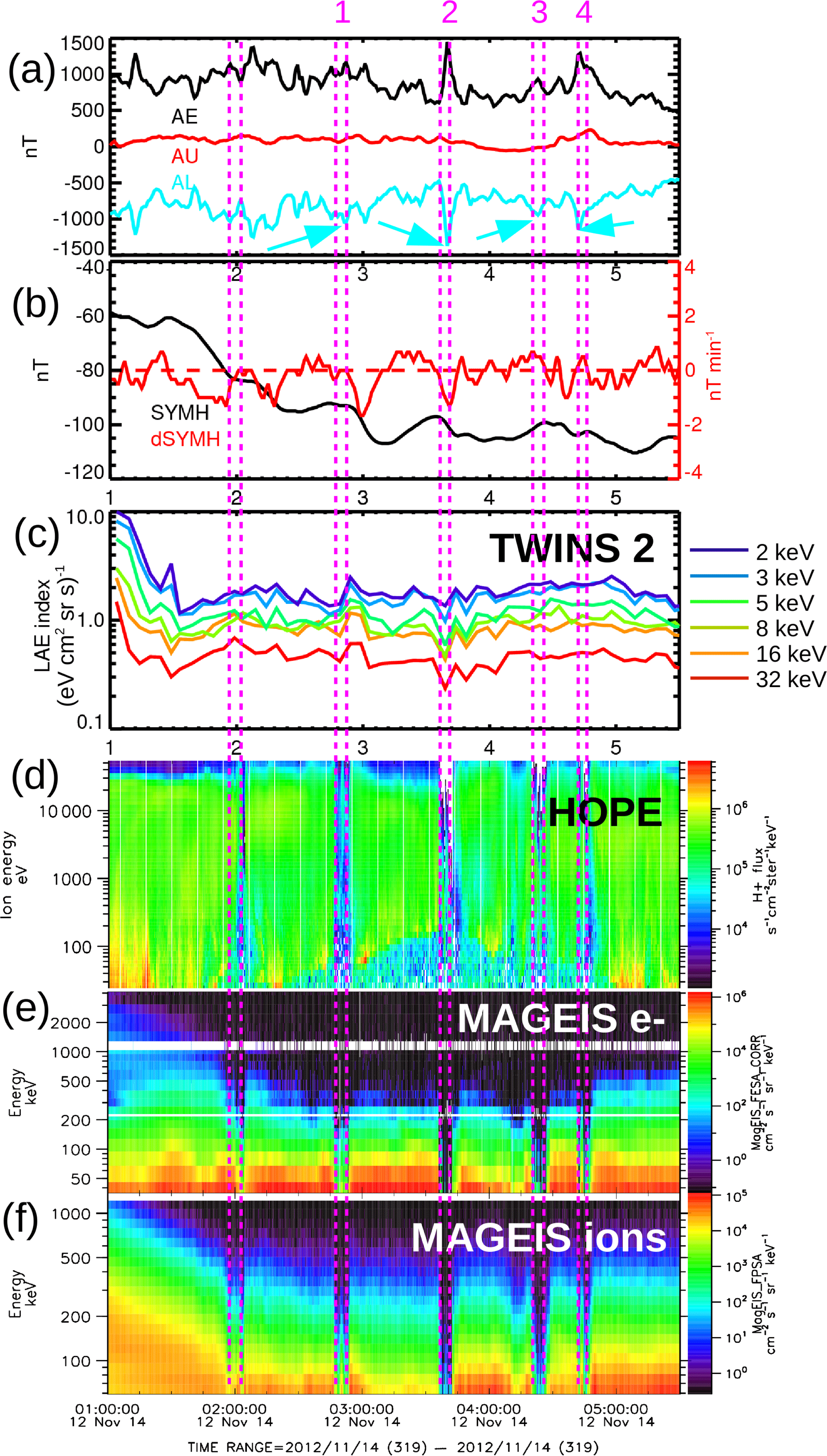
Figure 1 Overview of the dropout event for 14 November 2012. (a) Kyoto geomagnetic indices AE, AU, and AL; (b) Kyoto geomagnetic index SYMH and derived dSYMH; (c) TWINS 2 low-altitude emissions (LAEs) ENA index for multiple energy bands; (d) Probe A omnidirectional HOPE H⁺ fluxes in the energy range 20 eV–50 keV; (e) Probe A omnidirectional MAGEIS electron fluxes in the energy range 40 keV–4 MeV; (f) Probe A omnidirectional MAGEIS ion fluxes in the energy range 50 keV–2 MeV. The dropouts are marked by magenta lines. For the rest of the paper we will concentrate on the dropouts marked 1–4.

Figure 1 provides an overview of the dropout events that occurred during 01:00–05:30 UT on 14 November 2012. Geomagnetic indices are shown for geophysical context: Fig. 1a contains the AU, AL, and AE auroral indices, and Fig. 1b plots the SYMH and dSYMH ring current indices. Figure 1c shows the LAE index from TWINS 2 for several energy bands. Figure 1d to f show Van Allen Probe A flux spectrograms. Figure 1d plots HOPE protons (20 eV–50 keV). Figure 1e and f contain MAGEIS electrons (40 keV–4 MeV) and ions (50 keV–2 MeV), respectively.

From the previously reported observations, the dropouts have similar structure at Probe A and Probe B; however, there is a time lag of up to 5 min between the same structures appearing in Probe A and B data (Hw15, Di15). Here we include the data from Probe A only since the ≤ 5 min lag time is comparable to or smaller than the time cadences of TWINS ENA images (5 min) and AMPERE current maps (10 min). Following previous studies, we define dropouts in terms of crossing below a specific threshold of flux magnitude. This definition involves some ambiguity in the exact timing of dropouts because particle fluxes may drop before an actual boundary crossing owing to the finite gyroradius of the energetic particles used in sounding the boundary (Daly, 1982; Zong et al., 2004). Mitigating this concern, we note that dropouts with approximately the same timing were observed across a broad energy range. For each dropout observed by Van Allen Probe A during the period of interest, the start and end times of the dropouts are indicated in Fig. 1 by two dashed magenta lines, as derived from MAGEIS observations for high-energy particles. For the rest of this paper we concentrate on the dropouts labeled 1 through 4 at the top of Fig. 1. The dropout at about 02:00 UT is excluded from our analysis because TWINS ENA data were noisy at that time.

One characteristic feature of the Van Allen Probe dropouts is that they appeared in a broad energy range and were measured by all particle detectors for different species in the energy range from tens of eV (Fig. 1d; HOPE instrument) to MeV (Fig. 1e and f; MAGEIS instrument). Therefore, the occurrence of these structures seems independent of species type or energy, although there are some variations in morphology as a function of energy, species type, and pitch angle as reported by Hw15 and Di15. The dropouts contain complex substructures and have finite durations in time of approximately ∼ 5 to 10 min. These variations are explainable by spacecraft encountering different plasma populations when the OCB is crossed (Di15) and by finite gyroradius effects and boundary motion (Daly, 1982; Kettmann and Daly, 1988; Zong et al., 2004).

The LAE index (Fig. 1c) exhibits significant variations during and subsequent to the dropouts, especially during dropouts 1 and 2. For example, the 2 keV LAE index (blue line) increases from 1.5 to 2.7 (eV cm² sr s)⁻¹ during dropout 1, i.e., by more than 50 %. Similar increases are seen at other energies during dropout 1. During dropout 2, ∼ 50 % change is seen for a few energy ranges. Variations during dropouts 3 and 4 are present but not very pronounced. These significant variations in the LAEs indicate modulation of low-altitude ion precipitation that is correlated with the dropouts and observed at a distant magnetospheric location by Van Allen Probes.

The AU, AL, and AE indices also show considerable fluctuations during the periods of interest. For each dropout we identify an associated dip in the AL index (cyan arrows in Fig. 1a). Although there are dips in AL at other times when no dropouts are occurring, the AL dips during the dropouts are more pronounced. There are also measurable increases in the AE index at or near the times of each of the dropouts. The most pronounced AL dip or AE increase occurs for the dropout at ∼ 03:50 UT. These significant variations in the AL and AU auroral indices indicate modulation of the auroral electrojet, usually interpreted as a measure of substorm activity. Again, this ionospheric current modulation appears correlated with the dropouts occurring at magnetospheric altitudes.

The SYMH index (black) and its rate of change dSYMH (red) during dropouts are shown in Fig. 1b. SYMH decreased (indicating ring current intensification or injection) either during or shortly after each of the first two dropouts. During dropout 1, the rate of change of SYMH was close to 0 and after the dropout became negative. During dropout 2, the rate of change of SYMH was negative. A faster rate of ring current buildup during the main phase of the storm appeared right after dropout 2. In contrast, dropouts 3 and 4 occurred during SYMH recovery (positive rate of change).

The observations in Fig. 1 are summarized as follows. Particle flux dropouts were observed across a very broad energy range in the magnetosphere. These dropouts are temporally correlated with significant variations in low-altitude ion precipitation and geomagnetic indices for substorm activity and ring current injections. These correlations suggest global M–I coupling occurring at the time of the dropouts. More specifically, (i) for dropouts 1 and 2 there are more pronounced variations in the LAE index and a negative SYMH rate of change (ring current intensification or injection); (ii) for dropouts 3 and 4 the variations in LAE are less developed and the SYMH rate of change is positive; (iii) the most intense variation in the AL index is detected during dropout 2; (iv) the most intense negative SYMH rate of change is recorded shortly after dropout 1.

5 Analysis: TWINS ENA images and simulation results

In this section, we compare TWINS ENA images with images simulated by the global model for the dropout intervals. Whereas the LAE index is a proxy for global precipitation, ring current dynamics requires analysis of high-altitude ring current emissions (RCEs) and full ENA images.

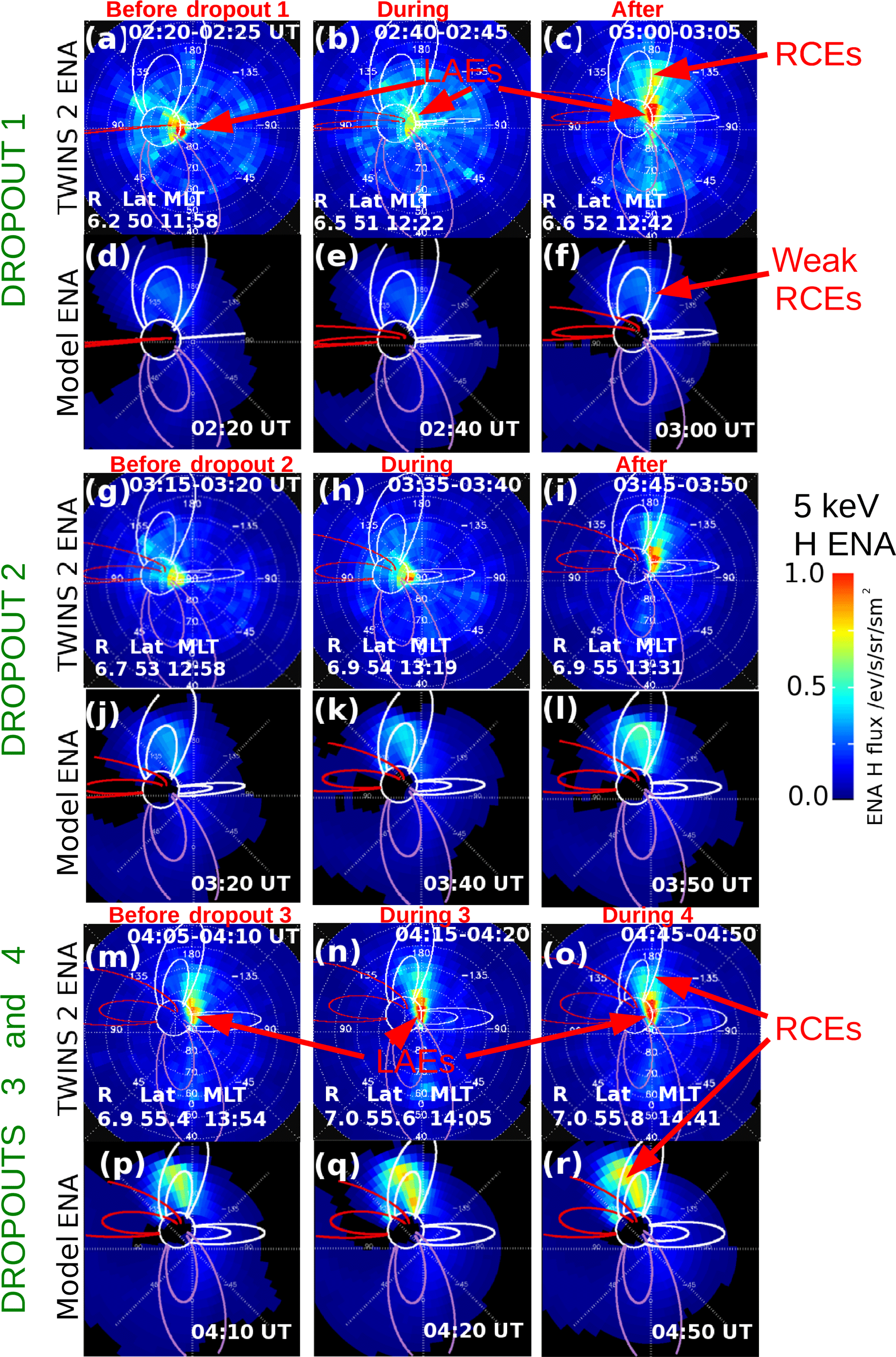
Figure 2 Dynamics of TWINS 2 ENA emissions and synthetic ENA images during the dropout intervals. Panels (a–c, g–i, m–o) show sky maps of TWINS 2 ENA differential fluxes in a fisheye projection for energy bin 5 keV ± 2.5 keV. Panels (d–f, j–l, p–r) show modeled ENA emissions plotted in the same projection. The field of view extends to 50^∘ from the center of the image. The limb of the Earth and dipole magnetic field lines for L=4 and 8 are drawn as guides. Noon (12:00 MLT) and dusk (18:00 MLT) field lines are colored red and purple, respectively. Low-altitude ENA emissions (LAEs) and high-altitude ring current emissions (RCEs) are marked by red arrows.

Figure 2 contains sky map (fisheye) projection images before, during, or after each of the dropouts (1 through 4). Each group of plots (dropout 1, dropout 2, or dropouts 3 and 4) shows three TWINS 2 ENA differential-flux images for the energy bin 5 keV ± 2.5 keV. Below each TWINS image is a corresponding simulated image for the same energy range. In each image the field of view extends to 50^∘ from the center of the image. The limb of the Earth and dipole magnetic field lines for L=4 and 8 are drawn as guides. Noon (12:00 MLT) and dusk (18:00 MLT) field lines are colored red and purple, respectively. For each TWINS image, the spacecraft location (radius, latitude, MLT) in SM coordinates is shown. Each TWINS ENA image is obtained with a 5 min integration time to accumulate a statistically significant number of counts in each pixel (Valek et al., 2010). Each corresponding synthetic ENA image is calculated for a particular snapshot time (indicated at the bottom) from the model. The same linear color bar is employed at all times for both TWINS 2 and synthetic images. The simulated ENA images include the contribution from the ring current ENAs only; i.e., they do not include the contribution from the LAEs, which are created in the optically thick region. LAEs and ring current emissions (RCEs) are labeled with red arrows.

We first focus on the TWINS 2 observations and save the discussion of the simulated ENA images for later. The time sequence is chosen to demonstrate the dynamics of both LAEs and ring current emissions as observed by TWINS 2 during Van Allen Probe dropout intervals. The ENA emissions before, during, and after dropout 1 are shown in panels (a–c) of Fig. 2. In each image, the LAE is the bright spot near the Earth limb. The LAE signal is strong: it peaks at ∼ 1 (eV cm² sr s)⁻¹ about 15 min before the dropout interval (panel a), becomes more localized and weaker right before the dropout (panel b), and returns to near its original flux level after the dropout (panel c). Although LAEs are known to have a highly directional emissivity, the modulation of the LAE signal during dropout 1 is most likely temporal and not caused by a change in viewing geometry. The LAE emissivity function has a broad peak about 12 h away from the imager and about 6 h wide in magnetic local time (Bazell et al., 2010; Goldstein et al., 2013, 2016). During the 02:20 UT to 04:50 UT period depicted in the entirety of Fig. 2 (not just the top panels for dropout 1) TWINS 2 moved from 11:58 MLT to 14:41 MLT, i.e., within 3 h at local time, and was well within the range for optimal viewing of the broad emissivity peak expected for nightside LAEs.

In addition to the LAE signal modulation, there is a clear ring current emission (RCE) in panel (c). Sharp changes in ring current ENAs between panel (b) and panel (c) are unambiguous evidence of a global ring current injection that occurred after dropout 1. However, we must explain why a ring current injection was not measured by Van Allen Probe A (Fig. 1). Our interpretation is that at the time of the dropouts, global magnetic field distortions were occurring that brought the OCB close to the Van Allen Probe A spacecraft. Van Allen Probe A was near the OCB, not in the trapped ring current.

Panels (g–i) of Fig. 2 show the ENA dynamics before, during, and after dropout 2. About 15 min after the 03:00 UT injection and ∼ 20 min before dropout 2 (panel g), both RCEs and LAEs become weaker. Right before dropout 2, the LAEs change their spatial structure and become more narrowly localized in MLT (panel h), from a previous MLT extent of about 2–3 h (panel c) to < 1 h. We note again that this change is most likely not caused by a change in viewing geometry, but rather a global narrowing of the spatial distribution of the peak ion precipitation. After dropout 2 (panel i), TWINS 2 observes a second ring current injection similar to that of 03:00 UT in panel (c). Panels (m–o) show the ENAs before dropout 3, during dropout 3, and during dropout 4. There are both clear ring current emissions and LAE emissions during 04:00–05:00 UT. The LAEs become weaker after the second injection (panels i and o) but the observed ring current emissions remain approximately steady both in intensity and in spatial structure.

Comparing the ENA images (Fig. 2) with the LAE index for different energies (Fig. 1), we note that the LAE index during dropouts 1 and 2 shows higher variability than the LAE index during dropouts 3 and 4. We also observe that after dropouts 1 and 2 were detected by Van Allen Probes, TWINS observed ring current injections that manifested as intensifications of high-altitude ENA emissions. During dropouts 3 and 4, the flux intensity of ring current ENA emissions remained approximately steady.

We now discuss the synthetic images (created from the BATS-R-US–CRCM simulation) shown for dropout 1 (panels d–f), dropout 2 (j–l), and dropouts 3 and 4 (p–r) in Fig. 2. As noted earlier, there is no calculation of LAEs in the synthetic images; therefore only the dynamics of ring current emissions will be compared. The synthetic ENA images show a continuous ring current buildup rather than the distinct injections observed by TWINS after dropouts 1 and 2. The model observes only a gradual, weak increase in RC flux from 03:20 to 03:50 UT (panels j–l). Simulated RCEs appear to stabilize to a quasi-stationary (in time) structure during the intervals of dropouts 3 and 4, which is consistent with the TWINS images.

The fact that modeled ring current structures are not as dynamic as those observed by TWINS agrees with previously published results (McComas et al., 2012). From the comparison between the model and TWINS observations we see that the modeled ring current shows much smoother behavior than the TWINS ring current that has both stronger and clearer injection signatures and faster decay. The magnitude of ENA fluxes for TWINS ring current emissions is in good correspondence with modeled fluxes on storm timescales. Therefore, although transport to the ring current in the real event seems more bursty, late in the main phase both the observations and the model results show similar levels of particle flux. As we will see from the comparison between AMPERE and the model results of the next section, there were structures in Birkeland currents during the intervals of the dropouts that can be interpreted as particle injections and that are connected with the same structures in the model results.

6 Analysis: AMPERE data and model results

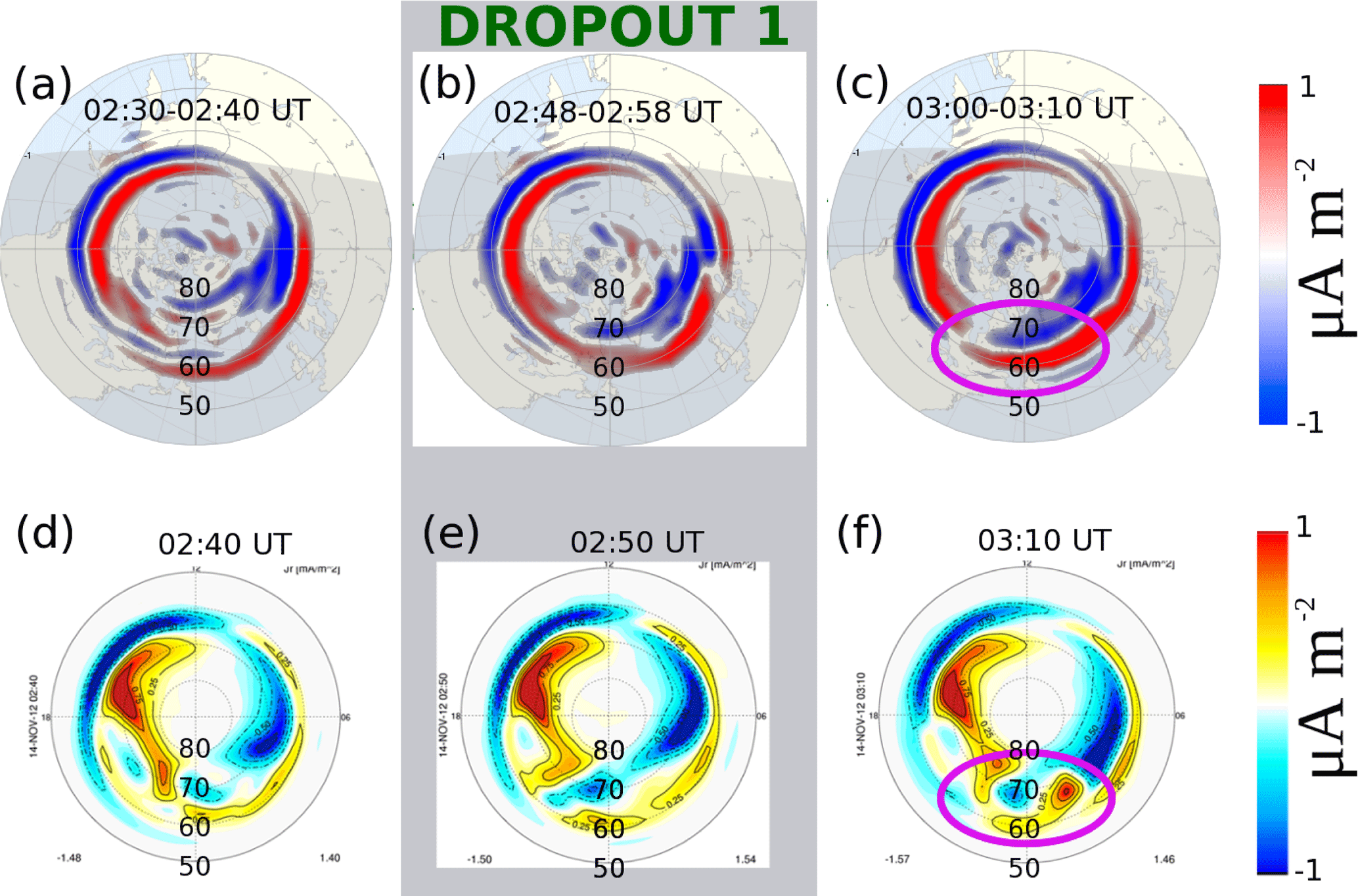
Figure 3 AMPERE-derived Birkeland currents and model Birkeland currents sampled to reflect dynamics before, during, and after dropout 1. The Birkeland currents J_r are calculated for the Northern Hemisphere. The units are µA m⁻²; color scale ranges from −1 to 1 µA m⁻². Noon is from the top of each panel, with dawn being from the right side and dusk from the left side. The grey rectangle denotes the panels corresponding to the dropout 1 interval from Fig. 1. The injection signature is denoted by the magenta oval.

Figure 3a–c show Birkeland currents calculated from AMPERE for three time intervals before, during, and after dropout 1. The Birkeland currents J_r are calculated for the Northern Hemisphere. The units of the color bar are µA  m⁻². Noon is at the top of the each panel, and dawn (dusk) is to the right (left). During this interval, Van Allen Probes were located in the dawn sector and TWINS 2 was on the dayside near noon MLT (Fig. 2). The grey rectangular region denotes the panels corresponding to the dropout 1 interval. In panel (a), both Region 1 (R1) and Region 2 (R2) current systems are observable, with a classical layered structure (R1–R2) seen mostly in the dusk and dawn regions. R1 currents near midnight are small in magnitude. R2 currents near midnight are evident and located mostly below 60^∘. During the dropout 1 interval (panel b), R2 field-aligned currents near midnight almost disappeared. After dropout 1, there is clear intensification of R2 currents near midnight, and the R2 current is located mostly above 60^∘. This intensification in R2 current enhancement coincides in time with the ENA flux intensification seen by TWINS after dropout 1.

Figure 3d–f show the modeled J_r from the BATS-R-US–CRCM simulation projected to the ionosphere and sampled at three different times before, during, and after dropout 1. The units and color bar are the same as for the AMPERE currents. The coordinate system is SM, which coincides with AACGM in the case of a pure dipole field at ionospheric altitudes. Though there are differences in the subglobal structures, the model globally reproduces both the current density (magnitude) and location of both the R1 and R2 systems. The model also reproduces the presence of layered R1–R2 structures in the dawn and dusk sectors, the lack of layered R1–R2 structure in the midnight sector (panels d and e), and the intensification after dropout 1 (magenta oval, Fig. 3f). In this same midnight-sector intensification region (magenta oval, Fig. 3f), the model produces a pair of upward–downward currents directly east–west of midnight MLT.

Figure 4 AMPERE-derived Birkeland currents and model Birkeland currents sampled to reflect dynamics before, during, and after dropout 2. The format is the same as for Fig. 4.

The same pattern is repeated for dropout 2 (Fig. 4) even more clearly. Figure 4a–c show AMPERE Birkeland currents sampled before, during, and after the dropout 2 interval. Figure 4d–f show the model-derived currents. There is a weak and irregular structure of currents in the midnight sector both for AMPERE and the model currents before and during the interval of dropout 2. After the dropout, both the data and the model show layered structures of R1–R2 currents in AMPERE data with intensification of R2 currents. The model also shows the bipolar structure of currents in the R1 with intensification of R2 currents.

The bipolar midnight current structure produced by the model is the result of particle injection in the two-way coupled code (Birn et al., 1996; Birn and Hesse, 1996; Buzulukova et al., 2010; Yang et al., 2012). We speculate that the absence of the clear bipolar signature and the layering of currents in the AMPERE data may be a manifestation of Hall reconnection (in the magnetotail), which is absent in the MHD equations used in BATS-R-US–CRCM. This speculation is supported by recent Hall and resistive MHD simulations of Ganymede's magnetosphere (Dorelli et al., 2015), which showed that the Hall effect modifies the symmetric structure of field-aligned currents in the reconnection region, and these changes affect the global convection pattern.

The comparison between AMPERE data and the model results provides a good opportunity to understand how the magnetospheric processes during the dropouts are represented by the coupled MHD–ring-current code. First, the structure of AMPERE currents for dropout 2 is very similar to that reported by Murphy et al. (2013) for the 16 May 2011 substorm (Fig. 10 from their work). Second, Murphy et al. (2013) pointed out that weakening of the FAC structure in the midnight sector is typical before a substorm onset. Pre-dropout FAC weakening is just what we observe, although more clearly for dropout 2, for which the AE substorm index was much stronger (∼ −1500 nT). Third, the strong intensification of the R2 current magnitudes (in both AMPERE and the model) is consistent with a ring current injection. Fourth, the TWINS-observed ENA flux enhancement is unambiguous evidence of a ring current injection. Taking into account these concordant observations and model results, we propose that dropouts 1 and 2 were associated with two magnetospheric substorms. We note that dropout 2 is correlated with a strong, well-defined spike in auroral indices, signifying an opportunity for a future study of the relationship between magnetotail structures, substorm onset, and the inner magnetospheric response.

Figure 5 AMPERE-derived Birkeland currents and model Birkeland currents sampled to reflect dynamics before, during, and after dropouts 3 and 4. The format is the same as for Fig. 4.

As we showed in the analysis of TWINS data, changes in ENA fluxes for dropouts 3 and 4 were not as dramatic as for dropouts 1 and 2. The AMPERE and modeled Birkeland currents are consistent with these TWINS ENA observations. Figure 5a–d show four maps of AMPERE Birkeland currents sampled to catch dynamics during and after dropouts 3 and 4. Four maps for model-derived currents are shown in Fig. 5e–h. Although there are some changes in the pattern during and after dropouts 3 and 4, the injection signatures are absent. In general, the pattern is more stationary, especially for the model-derived currents, and consistent with gradual ring current buildup during the main phase of the storm in the presence of quasi-stationary convection.

7 Interpretation and discussion

Previous studies from geosynchronous spacecraft related lobe encounters and corresponding particle dropouts to substorm activity (Thomsen et al., 1994; Moldwin et al., 1995; Kopanyi and Korth, 1995). Two recent papers (Hw15, Di15) reported dropouts observed by Van Allen Probes on 14 November 2012 and offered two different interpretations.

Hw15 studied the dropout intervals with data from Van Allen Probes, THEMIS, and GOES and argued that lobe boundary crossings cannot account for the dropouts because the B_y component of the magnetic field in the dropouts should be IMF dependent, which is not observed by Van Allen Probes. They suggest that the dropouts are flux ropes traveling from the tail reconnection site to the inner magnetosphere.

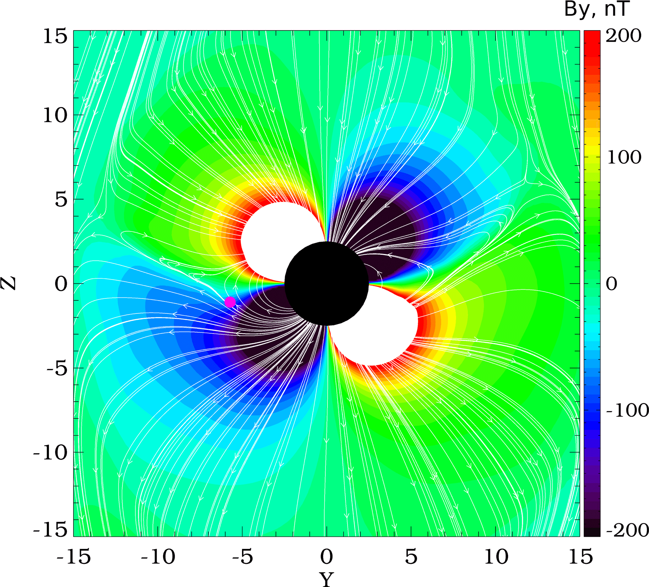
Figure 6 Color isocontours of model B_y (nT) in the GSM YZ plane (x=0) at 04:00 UT together with magnetic lines projected to the plane. Van Allen Probe A near 04:00 UT has the following GSM XYZ coordinates: 0.0;−5.65; − 1.17 R_E. The location of Probe A is denoted by the magenta circle. The effect of a thinner current sheet in the dawn sector is the effect of projection onto the YZ plane. These field lines are highly stretched in the tailward direction and appear near the OCB boundary.

To address this interpretation, in Fig. 6 we plot the B_y component in the GSM YZ plane (x=0) at 04:00 UT, with magnetic field lines (white) projected onto the GSM YZ plane and color indicating magnetic field strength (nT). At this time the Van Allen Probe A spacecraft was at GSM XYZ coordinates (0.0,−5.65, −1.17) R_E, as denoted by the magenta circle. The quadrupole structure of B_y near the Earth is a consequence of Earth's dipole field. (The effect of a thinner current sheet in the dawn sector is the effect of projection onto the YZ plane. These field lines are highly stretched in the tailward direction and appear near the OCB boundary). At larger geocentric distance, the B_y structure is strongly modulated by the IMF. Probe A was located in the region of near-Earth B_y quadrupole structure close to the Equator and also close to the OCB in the Southern Hemisphere. The satellite location is less than 1 R_E outside the region of open magnetic field lines and strong negative B_y up to −200 nT. The combination of the geometry of magnetic field lines and spacecraft location leads to strong negative B_y excursions when Probe A crosses the OCB in the Southern Hemisphere. The effect is independent of IMF orientation, at least in a first approximation, because the strong B_y field in this region is controlled by the Earth dipole. As shown by Di15, the HOPE observations indicate field-aligned particles traveling from the southern magnetic pole during the dropout, also confirming the lobe plasma population.

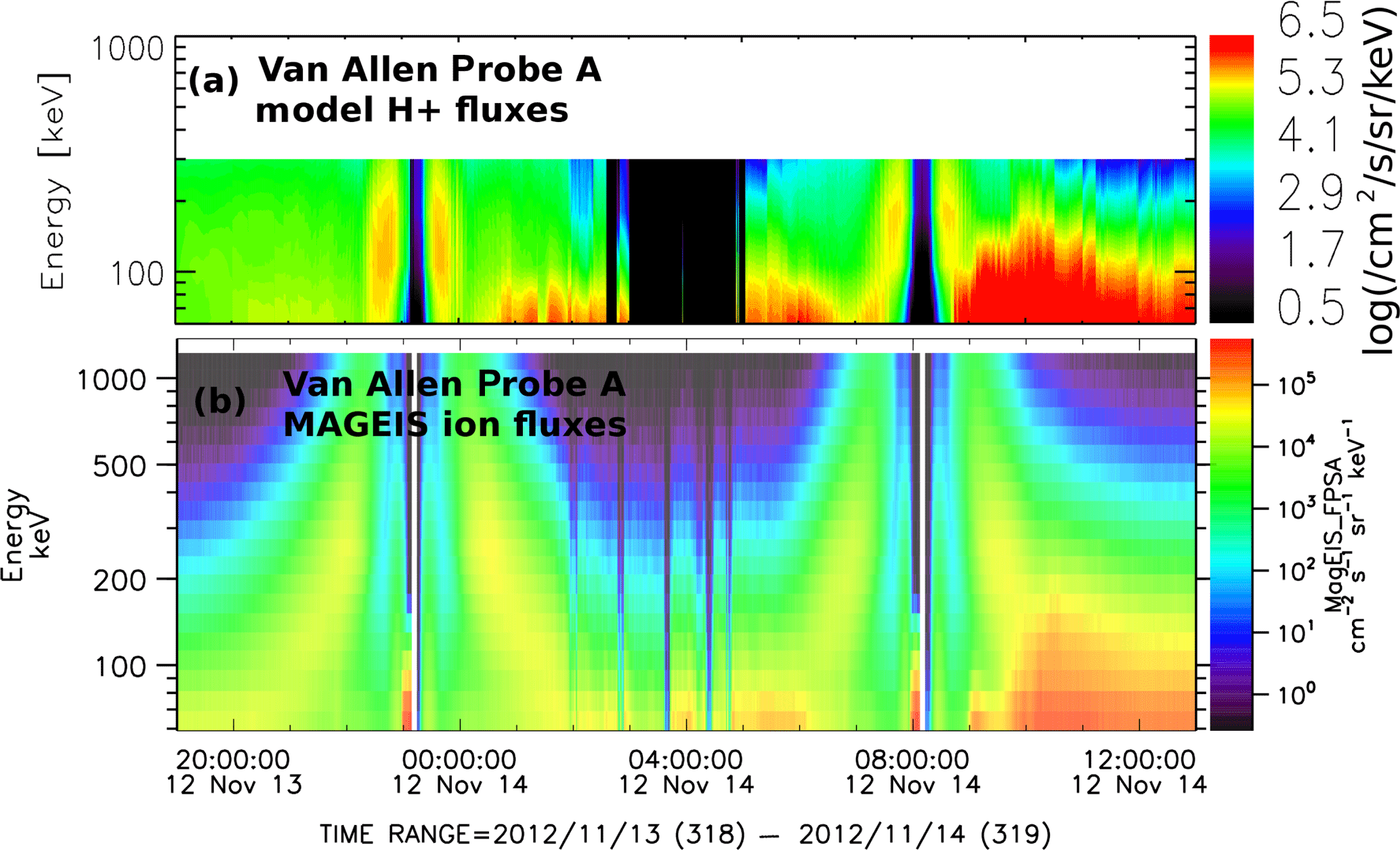
Figure 7 Modeled ion fluxes (a) along Probe A trajectory together with MAGEIS ion fluxes (b). The color scale is logarithmic. The units are cm⁻²/s/sr/keV for both panels. The black area between ∼ 03:00 and 05:00 UT in the modeled spectrogram denotes the modeled dropout.

The OCB distance from Van Allen Probes was calculated using the coupled BATS-R-US–CRCM model by Di15 with a model setup similar to the one we use for the present study. For both Probes A and B, the distance to the OCB oscillated from 01:05 UT through 05:00 UT and reached a minimum of 0.2 R_E for RBSP A at ∼ 04:30 UT (Fig. 8 from Di15). There was no OCB crossing by the virtual spacecraft in the model. However, because the spacecraft flew so close to the modeled OCB, we expect that dropouts should be visible in the ring current model results. Figure 7 shows modeled ion fluxes along the Van Allen Probe A trajectory (top) together with MAGEIS ion fluxes (bottom). The black area between ∼ 03:00 and 05:00 UT in the modeled spectrogram shows the modeled dropout, during which time the spacecraft was in the outer magnetosphere region beyond the CRCM-modeled polar boundary. This black region represents an interval favorable for dropouts to occur and is consistent with the calculations of the distance from the OCB performed by Di15. Although this modeled region is not a precise recreation of the dropouts because there was no OCB crossing, the virtual spacecraft did cross the CRCM polar boundary. This broad interval of modeled dropout cannot be explained by reconnection bubbles or the flux rope hypothesis; this is a geometrical effect caused purely by exiting the inner magnetosphere by crossing the CRCM-modeled polar boundary.

Di15 left unanswered the question of what caused the fluctuations of the OCB. From the analysis of the data and model results we conclude that dropouts 1 and 2 are related to substorm activity. Data showed the same pattern repeated for dropouts 1 and 2: namely, particle injection as seen by TWINS, weakening of FAC structure in the midnight sector before the dropouts, intensification of R2 currents in the midnight sector after the dropouts, and different SYMH rates of change (negative for dropouts 1 and 2). In addition, the model also predicted intensification of R2 currents and bipolar field-aligned currents interpreted as a substorm signature (Birn et al., 1996). Therefore, dropouts 1 and 2 are linked to OCB motion during substorm activity. This result is consistent with previous studies from geosynchronous spacecraft, in which the lobe encounters were explained by the reconfiguration of magnetospheric current systems and magnetic field lines during the growth phase of substorms. These changes are global, and local observation of the dropouts by Van Allen Probes is a manifestation of global magnetospheric reconfiguration. The ring current injections seen by TWINS are not observed in the Van Allen Probe data since spacecraft were located close to OCB and not in the inner magnetosphere, but substorm-related changes are causally related to both observations of the dropouts and ring current injections.

During dropouts 3 and 4, both TWINS and AMPERE data showed a relatively stable pattern with gradual ring current buildup and no signatures of injection or Birkeland current reconfiguration. These later two dropouts are interpreted as resulting from smaller motions of the OCB boundary not connected with global reconfigurations of field-aligned currents or particle injections (otherwise these structures would be observable in TWINS and AMPERE data). The remaining question is what caused the fluctuations of the OCB for dropouts 3 and 4? Since the OCB is defined as the topological boundary dividing regions between closed magnetospheric magnetic field lines and solar wind field lines (e.g., Glocer et al., 2016), any fluctuations in the interplanetary magnetic field will cause OCB fluctuations. The chance of observing the effect of these fluctuations will be higher if the spacecraft is located closer to the OCB. As reported by Di15, Van Allen Probe A in the model approached significantly closer to the OCB during dropouts 3 and 4 than during dropouts 1 and 2. We therefore suggest that before dropouts 1 and 2, the distance between spacecraft and the OCB was larger, and substantial disturbances (substorms) were needed to move the OCB to the spacecraft. Before dropouts 3 and 4, the distance between spacecraft and the OCB was minimal, and smaller disturbances were needed to achieve lobe encounters.

Our model results were used to interpret the data and choose between two different hypotheses, even though the model does not exactly reproduce all the measurements from different spacecraft in different regions of the magnetosphere. There are real, indisputable limitations of a first-principles model that takes solar wind data as an input and then simulates the data along a particular virtual spacecraft trajectory. However, we assert that the general, phenomenological, model-to-data concordance indicates that when combined with the observations, the model serves as a useful tool to link different processes in the magnetosphere and to aid interpretation. For example, the model does not reproduce ring current injections of the same strength as seen in TWINS data, but the modeled injection strength is sufficient to produce enhancement in R2 currents as seen by AMPERE. As a second example, the model cannot exactly reproduce OCB fluctuations at the location of the Van Allen Probes spacecraft, but it does show that the spacecraft were close to the OCB during the dropouts. Identification of such similarities – and discrepancies – leads to increased understanding and suggests future directions for improvements in the models.

8 Conclusions

We present a study of multipoint measurements by Van Allen Probes, TWINS, and AMPERE spacecraft with the two-way coupled global BATS-R-US–CRCM model in order to relate the particle dropouts in Van Allen Probe data to substorm activity and global M–I coupling.

1. For the two earlier dropouts (1 and 2), we find the following pattern: (1) weak nightside Birkeland currents before and during the dropout; (2) intensification of R2 currents after the dropout; and (3) particle injection detected by TWINS after the dropout. The model predicted similar behavior of Birkeland currents, indicating the occurrence of substorm activity related to these dropouts. TWINS low-altitude emissions demonstrated high variability during these intervals, indicating high geomagnetic activity in the near-Earth tail region.

2. For the two later dropouts (3 and 4), we find relatively stable Birkeland current structure and ENA emissions. The model also showed quasi-stationary behavior of Birkeland currents and ENA emissions with gradual ring current buildup, which is consistent with the storm main phase.

3. We interpret the first two dropouts as open–closed boundary (OCB) motion related to global changes in the magnetosphere during substorm activity and the second two dropouts as a result of smaller OCB disturbances when the distance between the OCB and spacecraft was minimal.

4. Although the model was not able to reproduce all dynamical features observed by TWINS or the exact OCB crossings by the Van Allen Probes spacecraft, we find that the multipoint analysis of the event together with the model results is very helpful in reconstructing the global picture.

Appendix A: Coupled model approach and setup

The near-Earth plasma region is described by multiscale physics reflecting a variety of processes and conditions in the complex, coupled magnetosphere–ionosphere system. To describe this system quantitatively, different physics domains should be described using different physical models (De Zeeuw et al., 2004; Ridley et al., 2004; Tóth et al., 2005; Fok et al., 2006; Moore et al., 2008). The global structure of the magnetosphere is well reproduced with magnetohydrodynamic (MHD) modeling. Global 3-D MHD models have proven to be an efficient tool for the description of the magnetosphere and its dynamic response to changing solar wind conditions. Several MHD codes, including BATS-R-US (Powell et al., 1999), LFM (Lyon et al., 2004), OpenGGCM (Raeder et al., 2008), and GUMICS (Laitinen et al., 2007), are widely used by the geophysical community. Global MHD codes for the Earth's magnetosphere are normally coupled with a separate ionosphere electrodynamics module to calculate the 2-D electric field patterns from the field-aligned currents at the MHD inner boundary.

In the inner magnetosphere, particles with mean plasma energy experience non-negligible or significant magnetic drift. Near-equatorial charged particles with energies in the range 1–200 keV and at distances of 3–10R_E are sensitive to this energy-dependent magnetic drift, which incurs an azimuthal drift that is oppositely directed for ions and electrons. In this situation the MHD assumption (single fluid with Maxwellian distribution function) fails, necessitating the inclusion of a “ring current model” into the global MHD code (De Zeeuw et al., 2004). A ring current model can be considered as a bounce-averaged kinetic code and normally operates with a large number (from hundreds to thousands) of “species”, i.e., distributed in energy, pitch angle, or first and second adiabatic invariants. Currently, there are several major ring current models used by the community: the standard Rice Convection Model (RCM) (Harel et al., 1981; Toffoletto et al., 2003) or the RCM-E, a version that includes frictional dissipation (Lemon et al., 2003; Chen et al., 2015); the Magnetospheric Specification Model (MSM) (Wang et al., 2003, 2004); the Comprehensive Ring Current Model (CRCM) (Fok et al., 1993, 1995, 2001, 2014) and its successor, the Comprehensive Inner Magnetosphere–Ionosphere model (CIMI) (Fok et al., 2014); the Ring current–Atmosphere interactions Model (RAM) (Jordanova et al., 1994, 2001, 2006) and its extended version with magnetic equilibrium solver (Zaharia et al., 2006; Zaharia, 2008); the Hot Electron and Ion Drift Integrator (HEIDI) code (Liemohn et al., 1999); and the Inner Magnetosphere Particle Transport and Acceleration model (IMPTAM) (Ganushkina et al., 2012).

For each species in a ring current model, an advection equation is solved with boundary conditions usually derived from empirical models for the electric field potential (Volland, 1973; Stern, 1975; Weimer, 2001) and plasma density and temperature (Tsyganenko and Mukai, 2003). A model magnetic field is specified in the simulation domain, e.g., the Tsyganenko family of models (Tsyganenko, 1995; Tsyganenko and Stern, 1996; Tsyganenko and Sitnov, 2005). A ring current model driven by empirical inputs is called a “stand-alone ring current model”. Stand-alone ring current models have been shown to adequately describe inner magnetosphere populations of H⁺, O⁺, He⁺, and e⁻ plasma with energies up to ∼ 200 keV at equatorial distances of 3–10 R_E at the magnetic equator (cf. the review by Ebihara and Ejiri, 2003, and the statistical survey by Wang et al., 2011). Two common drawbacks of these models are the lack of self-consistency between different inputs and a limited simulation domain.

A two-way coupled model combines an MHD code with a ring current model, allowing ring-current-induced electric and magnetic field feedback to the MHD code. A pressure correction to the MHD solution is calculated from the ring current model. Magnetic fields are calculated with ring current corrections (including the diamagnetic effect) and passed back to the ring current code. In this symbiotic approach, there are benefits for both components of the coupled system. For the ring current model, all inputs become self-consistent (i.e., no longer “stand-alone”); for a global MHD code, the inner magnetosphere description is better able to recreate the strong ring current buildup during geomagnetic storms and Region 2 Birkeland current intensifications. Recently developed versions of two-way coupled MHD–ring-current models have demonstrated their ability to quantitatively describe the global dynamics of the magnetosphere and inner magnetosphere and provide reasonable agreement with THEMIS ion fluxes, GOES magnetic field, and energetic neutral atom (ENA) maps from TWINS (Glocer et al., 2013).