Solar wind driving of the auroral outflow during the 23–26 September 1998 storm

Data from the FAST spacecraft are used to study the temporal progression of the energy inputs to the dayside cusp and the nightside aurora, including Poynting flux, electron number flux and amplitude of extremely low frequency (ELF) waves, during a storm driven by CME (Coronal Mass Ejections), and the resulting H⁺ and O⁺ outflows. The results show that (1) On the dayside, Poynting flux, ELF waves activity and soft electron precipitation are all enhanced during the initial and main phases of the storm, and decrease during the recovery phases. On the nightside, the Poynting flux increases during the initial and main phase, but the enhancements are smaller than on the dayside. The variations in the ELF wave activity and electron precipitation are similar before and during the storm. (2) The energy inputs are strongly correlated with the solar wind – magnetosphere coupling functions, $\mathrm{d}{\mathrm{\Phi }}_{\text{MP}}/\mathrm{d}t$ and $p^{\mathrm{1}/\mathrm{2}}\mathrm{d}{\mathrm{\Phi }}_{\text{MP}}/\mathrm{d}t$, especially in the dayside cusp region where the energy inputs and the ion outflows are localized. (3) The O⁺ and H⁺ ion outflow flux, $f_{{\mathrm{O}}^{+}}$ and $f_{{\mathrm{H}}^{+}}$, and the flux ratio $f_{{\mathrm{O}}^{+}}/f_{{\mathrm{H}}^{+}}$ all increase during the storm. Both the fluxes and the flux ratio reach their peaks on the initial phase and are enhanced during the main phase. Nightside auroral H⁺ and O⁺ outflows have lower outflow number fluxes than that in the dayside cusp region. These observations show how the solar wind changes characteristics of CME storms and results in strong sustained ion outflow during the initial and main phases.

1 Introduction

In the Solar wind–Earth's Magnetosphere–Earth's Ionosphere (S–M–I) coupled system, energy and momentum are transferred from the solar wind to the magnetosphere and ionosphere. However, the plasma of the magnetosphere is not only contributed by the solar wind. Plasma of ionospheric origin, including O⁺ ions, also populates the magnetosphere (Shelley et al., 1972; Geiss et al., 1978). The plasma from the solar wind as well as electromagnetic energy can penetrate to the ionosphere through magnetic reconnections in the dayside cusp (Peterson et al., 1998), heating and accelerating the ionospheric ions. The plasma of ionospheric origin gains energy and escapes from the Earth's ionosphere in both the dayside cusp region and the nightside aurora. Outflows can be either beams, which are correlated with field-aligned potential drops (McFadden et al., 1998; Möbius et al., 1998), conics, which show a significant correlation with wave activities and get energized through transverse heating (Lund et al., 2000), or polar wind (also called the ambipolar outflow), which consists of both low-energy ions and electrons that are moving along the field lines at high latitudes (Ganguli, 1996).

In recent years, statistical studies have been also carried out to investigate the dependence of the outflow on the solar wind and illumination (Yao et al., 2008; Peterson et al., 2006; Cohen et al., 2015), the storm time substorms (Nosé, et al., 2009), and the IMF control (Hatch et al., 2017). Using satellite observations, many studies have investigated the factors driving the escape of ions of ionospheric origin. Outflowing O⁺ ions are reported to be correlated to the energy inputs, including auroral electron energy deposition (Wilson et al., 2001), Poynting flux (Zheng et al., 2005; Strangeway et al., 2005), soft precipitating electrons (Strangeway et al., 2005), broadband extreme low frequency (BBELF) waves (Lund et al., 1999), and Alfvén waves (Chaston et al., 2007; Hatch et al., 2016). Using the FAST observations in the dayside cusp region during a geomagnetic storm, Strangeway et al. (2005) evaluated the relations between the outflowing ions, measured by the ESA instrument, and the energy inputs. They found that the Poynting flux and the electron density are the best controlling factors. Empirical models are also given in their study. Similar results were found by Zheng et al. (2005), using multi-instrument data from the Polar satellite. Wave-particle interactions allow ions to gain energy. At medium altitudes between 2000 and 4000 km, ions are more preferentially heated by BBELF waves than EMIC waves, which are correlated with the acceleration of He⁺ ions (Lund et al., 1999). Using FAST/ESA observations, Kitamura et al. (2021) found that the dependence of the outflow flux on Poynting flux is not significantly affected by the solar illumination but the slope of the dependence on precipitating electron density decreases with the solar zenith angle.

Recent work has used a recalibrated FAST/TEAMS dataset to examine how the outflow of O⁺ and H⁺ vary during geomagnetic storms. Nowrouzi et al. (2023) used a solar cycle of FAST data to examine how the outflow varies with storm phase for different types of storms. They found that for both CME (coronal mass ejections) and SIR (streaming interaction regions) storms, the outflow peaks in the main phase, and declines, but is still significant, in the recovery phase. In addition, they found that for CME storms, there was a strong increase in outflow during the initial phase that was not observed for SIR storms. Zhao et al. (2020) and (2022) examined the correlation between energy inputs and O⁺ and H⁺ outflow flux in both the dayside cusp region and the nightside auroral region for one CME-driven storm, the 24–25 September 1998 storm event. This is the same event examined by Strangeway et al. (2005). Consistent with the findings of Strangeway et al. (2005), the Poynting flux and the soft electron are strongly correlated with both the O⁺ and the H⁺ outflows in the cusp region. However, the best controlling factor for O⁺ is the Poynting flux (r=0.85) while the H⁺ outflows correlate best to the electron number flux (r=0.76). In the nightside auroral region, Zhao et al. (2022) found that O⁺ outflow is correlated with both Poynting flux and electron precipitation while H⁺ outflow is only correlated with electron precipitation on the nightside.

Thus, we know that the outflow changes significantly during a storm, and we know that both precipitating electrons and electromagnetic energy input play roles in driving the outflow. The outstanding link in the chain is to understand the driving factors in the solar wind that best control the energy input, leading to the storm phase-dependent ion outflow. A recent paper (Hull et al., 2023) examined the chain of energy flow using Cluster data in the cusp and Wind in the solar wind. They found that pressure enhancements in the solar wind and northward excursions of the IMF were associated with enhancements in Alfvén wave activity and plasma, which then led to enhanced O⁺ outflow. However, this study was for just one pass during the main phase of a storm, and did not address how the range of parameters that can occur in the solar wind will drive outflow. If we understand which solar wind and IMF parameters lead to the enhanced energy input that then leads to outflow, and how these parameters change during a storm, we can use this knowledge to better predict storm development.

To supplement our previous work on the correlations between energy input and ion outflow, this work takes the additional step to address the changes in the solar wind that correlate best with the energy inputs into the aurora. The solar wind and IMF are driving the energy input into the aurora region, and the energy input then drives outflow. That outflow then flows along the field and, depending on convection, may end up closer or further down the field. Papers have addressed the correlations between the solar wind input and the outflow flux (e.g. Lennartsson et al., 2004; Peterson et al., 2024), and between the solar wind input and the total escape rate (e.g. Schillings et al., 2019; Ramstad and Barabash, 2021). But there are still questions on the direct connection between the solar wind parameters (pressure, B_z, etc) and the resulting energy flux, both Poynting and precipitation, into the auroral zone.

In this paper, we again use the 24–25 September 1998 CME-driven storm event to examine the changes that are observed in the solar wind and IMF as the storm progresses, and how those are related to the changes in the energy input and the outflow in the cusp and nightside auroral regions. In particular, we will address: (1) How do the energy input and the outflow flux change with time during the storm? (2) Which solar wind drivers are responsible for the enhanced energy input? In Sect. 2.1, the 24–25 September 1998 geomagnetic storm will be reviewed in brief. In Sect. 2.2, the FAST/TEAMS measurement is introduced, and the data sets of this study are shown. In Sect. 2.3, we introduce how we calculate the parameters. Results will be given in Sect. 3, where the proposed questions will be discussed in Sect. 3.1–3.4. Discussion and conclusions are given in Sect. 4.

2 Methodology

2.1 Overview of the geomagnetic storm

An interplanetary shock from a large CME arrived at the Earth's magnetopause with a space speed of 769 km s⁻¹ at 23:45:00 UT on 24 September 1998 (Russell et al., 2000). It was observed at 25 September 1998/00:00:00 UT by the FAST satellite when it entered the dayside cusp region, 16 min later. During the storm, the Earth's magnetopause was moved inward and the dayside magnetospheric boundaries are pushed tailward. Significant energy was injected into the ionosphere in both the dayside cusp region and the nightside auroral oval zone, producing remarkable outflows. The storm, which occurred during the rising phase of solar cycle 23, had a solar radio flux at 10.7 cm wavelength (F10.7) between 136.2 and 144.1 s.f.u. (${\mathrm{10}}^{-\mathrm{22}}\mathrm{W}({\mathrm{m}}^{\mathrm{2}}\mathrm{Hz}{)}^{-\mathrm{1}}$) from 23–26 September 1998.

Figure 1A panels (a–c) show the interplanetary magnetic field (IMF) and the solar wind dynamic pressure (P_dyn) propagated to the Earth's magnetopause. IMF first turns northward and starts to show strong perturbations at around 24 September 1998/23:45:00 UT. The IMF B_z component alternates between northward and southward, fluctuating between 20 and −20 nT. Meanwhile, the Dst index (panel e) sharply increases by 45 nT after the pulse of the shock, indicating the SSC. The IMF B_z component (panel b) reaches its first minimum of −20 nT at 25 September 1998/00:21:30 UT, when the solar wind dynamic pressure approaches its first peak value of 14 nPa. The Kp index is 7⁺ at the sudden storm commencement (SSC), as shown in panel (g). Panel (h) shows the quantity $\sin ({\mathit{\theta }}_{\mathrm{c}}/\mathrm{2})$, an indicator of the southward orientation of the IMF, with 1 for a purely southward field and 0 for a northward field. Panels (i) and (j) show two solar wind-magnetosphere coupling functions $\mathrm{d}{\mathrm{\Phi }}_{\text{MP}}/\mathrm{d}t$ and $p^{\mathrm{1}/\mathrm{2}}\mathrm{d}{\mathrm{\Phi }}_{\text{MP}}/\mathrm{d}t$, from Newell et al. (2007). The first,

$${\displaystyle \frac{\mathrm{d}{\mathrm{\Phi }}_{\text{MP}}}{\mathrm{d}t}}=v^{\frac{\mathrm{4}}{\mathrm{3}}}{B}_{\mathrm{T}}^{\frac{\mathrm{2}}{\mathrm{3}}}{\sin }^{\mathrm{8}/\mathrm{3}}\left({\displaystyle \frac{{\mathit{\theta }}_{\mathrm{c}}}{\mathrm{2}}}\right),$$

combines the information from the rate IMF field lines approaching the magnetopause (proportional to the solar wind speed v), the percentage of the field lines merging (proportional to ${\sin }^{\mathrm{8}/\mathrm{3}}({\mathit{\theta }}_{\mathrm{c}}/\mathrm{2})$, where θ_c is the IMF clock angle), and the length of the merging line (proportional to $(B_{\text{MP}}/B_{\mathrm{T}}{)}^{\mathrm{1}/\mathrm{3}}$, where B_T is the IMF magnitude and B_MP is the field magnitude at the magnetopause), to give an approximation to the rate magnetic flux is opened at the magnetopause. This function has been found to correlate well with many indicators of geomagnetic activity. The second function, which is scaled by the dynamic pressure, was found to have a better correlation with Dst (Newell et al., 2007). As shown in the plot, multiple parameters change during the storm. B_z drops significantly during the storm main phase, while the dynamic pressure increases significantly. In addition, the intensity of both coupling functions increase during the initial phase of the storm, remain enhanced during the main phase, and decline during the recovery phase. In Sect. 3.4, we will calculate the correlations between the different drivers that change on storm time scales and the energy inputs to discuss the factors driving the energy inputs to the ionosphere, which accelerate ions to outflow.

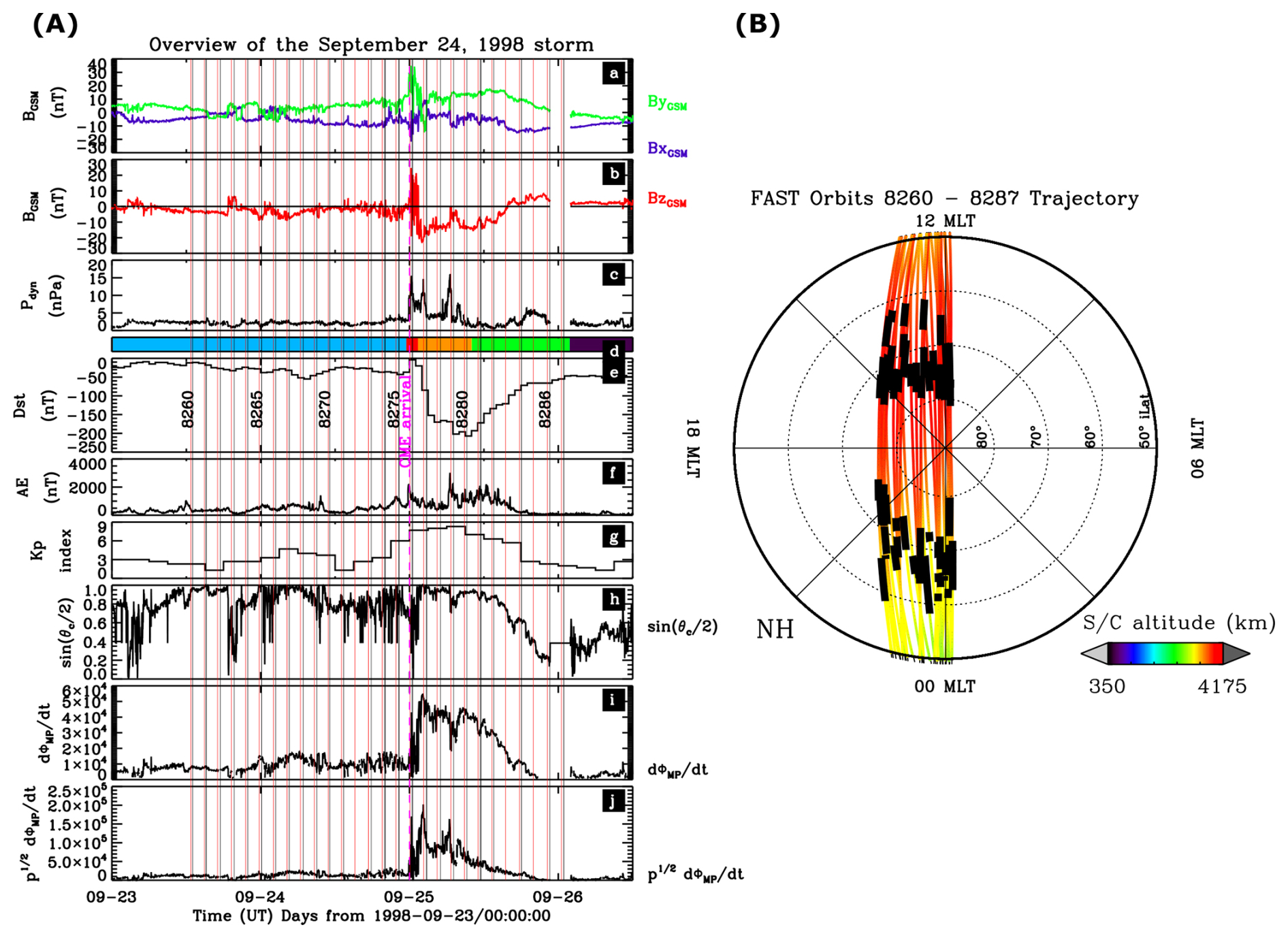
Figure 1 Left-hand plot (A): overview of the storm. From top-down, the plot shows (a) the interplanetary magnetic field B_x and B_y, (b) B_z, (c) the solar wind dynamic pressure, (d) the color code of the storm phase (blue for pre-storm times, dark red for the initial phase, orange for the main phase, and green for the recovery phase), (e) the Dst index, with some orbit numbers labelled at the vertical lines which indicate the start times of the dayside outflows (in red) and the nightside outflows (in black), (f) the AE index, and (g) the Kp index, (h) $\sin ({\mathit{\theta }}_{\mathrm{c}}/\mathrm{2})$, where θ_c is the IMF clock angle, (i) the rate magnetic flux is opened at the magnetopause, $\mathrm{d}{\mathrm{\Phi }}_{\text{MP}}/\mathrm{d}t$, and (j) $p^{\mathrm{1}/\mathrm{2}}\mathrm{d}{\mathrm{\Phi }}_{\text{MP}}/\mathrm{d}t$, where p is the solar wind dynamic pressure (Newell et al., 2007). The magenta vertical line indicates the time of the coronal mass ejection (CME) arrival. Right-hand plot (B): trajectories of the 28 FAST orbits. The coordinate system is magnetic local time by magnetic invariant latitude. The Sun is in the upward direction. The bolded segments represent the time intervals when outflows are observed in either the nightside auroral oval zone or the dayside cusp region, as Strangeway et al. (2005) did but they used 33 orbits and considered data acquired only on the dayside. The color code indicates the spacecraft altitude above the Earth's surface.

The FAST spacecraft was traveling through the dayside cusp region over the polar cap to the nightside auroral oval zone, observing a large amount of H⁺, He⁺, and O⁺ outflows. The arrival time of the coronal mass ejection, during orbit 8276, is marked by the magenta vertical line in Fig. 1A (see Strangeway et al., 2005 and Zhao et al., 2020 for the summary plot of this orbit).

2.2 Instrumentations and data sets

Fast Auroral Snapshot Explorer (FAST) travels through the auroral oval four times each orbit (133 min orbital period) at altitudes from 350–4175 km, due to its orbit configuration with a high inclination angle (83°). It was designed to study the particle transportations and accelerations in the polar ionosphere, providing measurements of the electric and magnetic fields, plasma waves, energetic particles including electrons and ions, ion composition, and the density and temperature of plasma with a high temporal (microseconds) and spatial resolution (Pfaff et al., 2001; Carlson et al., 2001; Ergun et al., 2001; Elphic et al., 2001; Klumpar et al., 2001), allowing us to study the process of the outflows, electric currents, and plasma waves in the magnetosphere-ionosphere coupling system. There are four scientific instruments and an instrument data processing unit (Harvey et al., 2001; Pfaff et al., 2001).

This study uses the data from all the instruments. The Electrostatic Analyzer (ESA) measures the electron (eESA) and ion (iESA) distribution function over a 180° of field of view (FOV) in 48 energy channels and 32 pitch-angle bins every 78 ms (Carlson et al., 2001). The measured energy ranges from 4 eV–32 keV for electrons and 4 eV–25 keV for ions. The Electric Field Sensors (Ergun et al., 2001) and the Magnetic Field Experiment sensors (Elphic et al., 2001) measure electric field data, plasma density, and temperature, and magnetic field data. The electric field covers frequencies from DC (0 Hz) to ∼2 MHz. The AC magnetic field data spans frequencies from 10 Hz–500 kHz. The TEAMS instrument measures the full 3D distribution function of the major ion species (including H⁺, He⁺, O⁺) with an instantaneous 360×8 field of view with energies between 1 eV charge⁻¹ and 12 keV charge⁻¹. The time resolution depends on the mode of the instrument. At the fast-sampling mode, the data is transmitted to the ground every 2.5 s (a half spin period), while the data is transmitted every 10 or 20 s (2 or 4 spins) for H⁺ and O⁺ in slow modes (Klumpar et al., 2001).

Recently, the TEAMS instrument has been recalibrated by similar methods to those used for the similar Cluster/CODIF instruments (Kistler et al., 2013). The calibration methods are described in Zhao et al. (2022), Lund et al. (2025), and the appendix section of Nowrouzi (2022). This study uses the level 2 pitch-angle energy product for the TEAMS analysis. In particular, the level-2 TEAMS data have been corrected for spacecraft potential to ensure that the calculated outflow flux of the low-energy ions is less affected by the spacecraft charging. The data is also transformed to the E×B plasma frame to eliminate effect by the spacecraft motion, which distorts particularly the distribution of low-energy ions, the so-called ram effect. The level 2 datasets are available at the NASA Space Science Data Center (NSSDC).

FAST observations are selected during the period from 12:00:00 UT on 23 September 1998 to 01:00:00 UT on 26 September 1998. There are 28 orbits during the period, with 16 orbits before the storm, 1 orbit during the initial phase, 4 orbits during the main phase, and 7 orbits during the recovery phase. The start times of the dayside outflows and the nightside outflows are marked by the red and black vertical lines, respectively, in Fig. 1A. The trajectories during this time are near the noon-midnight meridian plane, covering the cusp region and the nightside aurora. Outflows, including both H⁺ and O⁺, are observed by FAST in those regions, allowing us to investigate the change in the outflows with time from the dayside cusp and nightside aurora zone and make a comparison between the two source regions. Figure 1B shows the trajectories of the orbits in this study. The outflow time intervals are shown in bold lines. The method used to identify the outflow time intervals is described in Zhao et al. (2022). Some orbits show multiple bold intervals because the nightside outflow is not continuous and can occur at multiple latitudinal locations. The source region of the outflows has good coverage in magnetic local time (MLT) from 21:00 to 01:00 UT, and in ILAT from 60–80°. There are a total of 865 (1114) spin-averaged measurements (the spin period is 5 s at the fast mode) for O⁺ and H⁺ collected by the TEAMS instrument in the nightside (dayside) source region. All observations are collected above 2500 km altitude, and more than 92 % are collected between 3000 and 4000 km. The average altitude is ∼3400 km (∼4100 km) for the observations on the nightside (dayside). All fluxes, including the H⁺ and O⁺ outflow number flux, the Poynting flux, the electron energy flux, and the electron number flux, are mapped to 100 km.

The FAST field instruments can measure the electric field components E_x, E_z and the magnetic field $\mathit{B}=(B_x,B_y,B_z)$. The E_x component is along the spacecraft velocity in the northern hemisphere (in the southern hemisphere, it is anti-parallel to the spacecraft velocity) and E_z is near the magnetic field direction at high latitudes. The three components of the magnetic field are determined in both the spacecraft spin plane coordinates (B_sc) and the geocentric equatorial inertial coordinates (B_gei). The difference in the magnetic field, δB, is calculated in field-aligned spacecraft coordinates, with δB_x along the spacecraft velocity vector, along track, δB_y in the direction of B cross spacecraft velocity vector, across track, and δB_z along the model magnetic field B. This study focuses on the downward Poynting flux, $S=E_x\cdot \mathit{\delta }{B}_y/{\mathit{\mu }}_{\mathrm{0}}$, where μ₀ is the permeability of vacuum.

2.3 Calculations of the energy-input parameters and the outflow flux

The parameters analyzed in this study include (1) the number flux of the individual ion species, H⁺ and O⁺, recorded as $f_{{\mathrm{H}}^{+}}$ and $f_{{\mathrm{O}}^{+}}$, respectively, (2) the amplitude of the extremely low frequency (ELF) waves, recorded as A_elf, (3) the quasi-static Poynting flux, S_dc, (4) the Alfvénic Poynting flux, S_ac, and (5) the electron number flux, f_en. We also use P_dyn, B_Z, and the two Newell et al. (2007) coupling functions to analyze the correlation of between the energy input and the solar wind parameters.

The outflow flux and the energy input parameters are determined from the FAST data by the same method as described in Zhao et al. (2020, 2022). The outflow number flux is calculated by integrating the differential energy flux aligned to the field line over energy and over pitch angle. The energy is integrated from 1 eV to a dynamic energy, E_dyn, which separates the outflowing ions from the isotropic ions of plasma sheet origin (see Hatch et al., 2020, for details of the method). The pitch angle ranges from 0–180° so that it gives the net flux. The ELF waves cover the frequencies from 32 Hz–16 kHz, a combination of the very low frequency (VLF) and the ELF bands (Ergun et al., 2001). The amplitude of the waves is calculated by integrating the electric field power density over the frequencies covering the band from 32 Hz–16 kHz collected from 118 frequency channels. Thus, the band covers high-frequency Alfvén waves, oxygen and hydrogen cyclotron waves, low-frequency whistler mode waves, and BBELF waves. The eESA data is used to determine the electron number flux. The electron fluxes are integrated over energies above 50 eV to exclude the photoelectrons. This threshold value was used by Strangeway et al. (2005), and we are following them. Observations also show significant fluxes by photoelectrons below 60 eV in the FAST altitudes (Peterson, 2021). The despun magnetic field (Strangeway et al., 2005) is sorted into two frequency bands, 0.125–0.5 Hz, corresponding to the fluctuations of Alfvénic waves, and <0.125 Hz, corresponding to the quasi-static fluctuations. Thus, the DC Poynting flux, S_dc, is associated with the fluctuations below 0.125 Hz, while the Alfvénic Poynting flux covers the frequencies of 0.125–0.5 Hz.

We first determine the time intervals of the outflows by the method described in Zhao et al. (2022). Once the time intervals are determined, averages or maxima are calculated for all the quantities over the time interval. In this study, averages are obtained for the outflow fluxes, the electron number flux, and the amplitude of ELF waves, while maxima are computed for the Poynting fluxes since we found that the Poynting flux is concentrated spatially in a narrow region compared to the selected wide range for outflows. We integrate and average the solar wind parameters from the previous hour prior to the outflows observed by the FAST satellite to include a more integrated picture of the energy input. The beginning and ending times of the outflowing intervals are the same as Zhao et al. (2022). The day side picks up the cusp and surrounding region broadly, while the night side picks up only a small part of the auroral zone where significant outflows are observed. In the 28 FAST orbits (numbered from 8260–8287), there are 5 orbits on the nightside (8272, 8283; 8270, 8271, 8278) and 5 orbits on the dayside (8260, 8270, 8271, 8272, 8280) with no TEAMS observations (the instruments were off during the time period) or with significant TEAMS data gaps during the outflow time period. These time periods are not used for the TEAMS data. There are a few orbits on the nightside with multiple outflow regions, and we use the most poleward region, which has the largest outflow. In addition, the nightside H⁺ number flux is too low in orbit 8285, so that time period is deleted from our study. Thus, we have 23 outflow time periods on the dayside and 22 outflow time periods on the nightside. The iESA data and the energy input data are available for all 28 orbits. With these samples, the questions proposed in the introduction section will be discussed in the following sections.

3 Observations

3.1 Sample orbits during the storm

Figure 2 shows the data quantities of this study for three orbits: orbit 8275 (left panel (A)), before the SSC of the storm, orbit 8277 (middle panel (B)), two hours after the SSC, and orbit 8279 (right panel (C)), towards the end of the main phase, indicating the progression during the storm. FAST was moving through the dayside cusp region over the polar cap and over the nightside auroral oval zone during each orbit, as shown at the far right in the plot. For each orbit, the panels, from top to bottom show (a) electron spectrograms from the eESA instrument, (b) omnidirectional ion spectrum from the iESA instrument, (c and d) H⁺ and O⁺ omnidirectional energy spectra from the TEAMS instrument, (e and f) pitch angle distributions of H⁺ and O⁺ integrating from 1–500 eV, (h–k), the DC Poynting flux, the Alfvénic Poynting flux, the electron number flux, and the amplitude of the ELF waves. Panel (l) shows the ion outflow flux for the three species H⁺, O⁺, He⁺, as well as the all-ion outflow flux from the iESA instrument. We note that there are significant differences between the iESA instrument and the TEAMS instrument. Their minimum energy is slightly different, the iESA measures a 2D distribution while TEAMS measures the full 3D distribution, the iESA is more susceptible to penetrating electron background, and TEAMS requires a large dead time correction during high fluxes, which leads to a larger uncertainty. Thus, we do not expect the two measurements to be identical, but we certainly expect them to show the same trends.

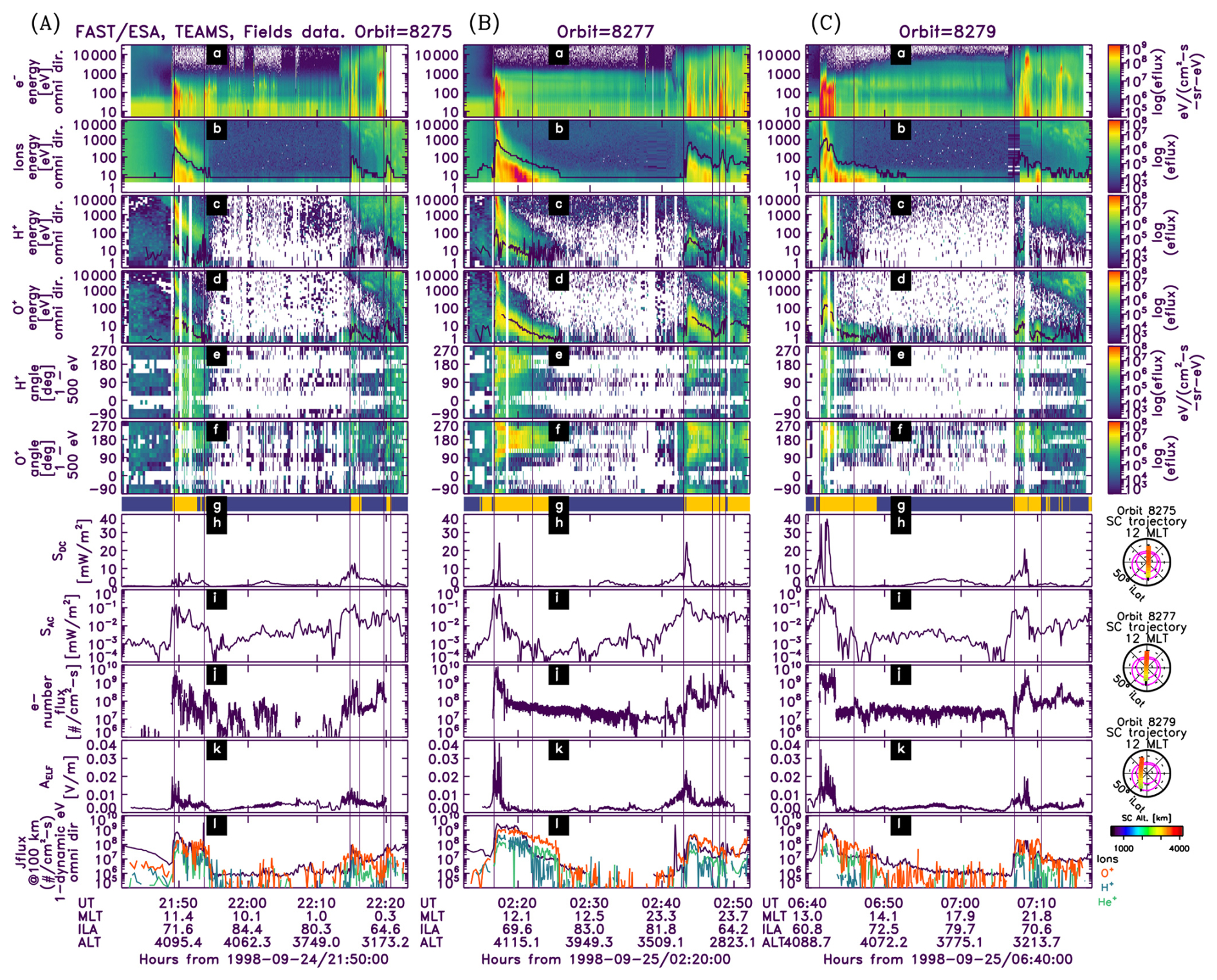
Figure 2 The FAST observations in orbit 8275, left panel (A), before the storm sudden commencement (SSC), orbit 8277, middle panel (B), during the main phase of the storm, and orbit 8279, right panel (C), near the end of the main phase. From top down, this plot shows (a) the electron energy-time spectrogram, (b) the ions energy-time spectrogram, with the cutoff energy (black line) superimposed determined by the ESA instrument, (c) the TEAMS H⁺ energy-time spectrogram with the characteristic energy (black line) superimposed, (d) the TEAMS O⁺ energy-time spectrogram with the characteristic energy (black line) superimposed, (e) the TEAMS H⁺ pitch angle spectrogram for energies between 1 and 500 eV, (f) the TEAMS O⁺ pitch angle spectrogram for energies between 1 and 500 eV, (g) the outflow bar, showing the outflow time interval with yellow, (h) the quasi-static Poynting flux, (i) the Alfvénic Poynting flux covering frequencies of 0.125–0.5 Hz, (j) the 50 eV–35 keV electron number flux, (k) the amplitude of ELF waves covering frequencies of 32 Hz–16 kHz, (l) the field-aligned number flux $f_{{\mathrm{O}}^{+}}$ for O⁺ (red), $f_{{\mathrm{H}}^{+}}$ for H⁺ (blue), and $f_{{\mathrm{He}}^{+}}$ for He⁺ (green). The outflow flux measured by iESA is overplotted (black line). Data will be averaged over the outflow time in the dayside cusp (the first couple of the vertical lines), the poleward segment of the nightside aurora (the second couple of the vertical lines), and the equatorward of the nightside aurora (the third couple of the vertical lines). The trajectories of the three orbits are shown in the right-side small dial plots, with the magenta line indicating the empirical location of the auroral oval zone.

The first orbit illustrates the energy input and outflow during a relatively quiet time. The plot shows the passage through cusp from ∼21:49–21:53 UT and the passage over the nightside aurora from ∼21:14–21:21 UT. The cusp has two ion populations, a higher energy latitude-dispersed population that is predominantly H⁺ and a lower energy population that is predominantly O⁺. The high-energy population is the magnetosheath population entering through reconnection (Peterson et al., 1998). The latitude dispersion is due to a time-of-flight effect due to the tailward convection of the reconnected field line, with higher energy ions entering earlier than lower energy ions (Connor et al., 2015). The pitch angle distributions show that the low energy population consists of upflowing conics. The nightside aurora also shows two ion populations. In this case, the higher energy population is the plasma sheet precipitating or mirroring at low altitudes. The low energy population is dominantly O⁺ and has a conic distribution. Panels (h)–(k) show that in both the cusp and nightside auroral regions, the DC and AC Poynting flux, the precipitating number flux, and the EFL amplitude are enhanced. The resulting outflow from the upflowing conic distributions is seen in panel (l). This shows that even prior to a storm, during relatively quiet time, there is energy input and outflow in the cusp and auroral regions. The next two orbits show the changes during the storm. In orbit 8277, after the SSC, the DC and AC Poynting flux and precipitating electrons are all enhanced, particularly close to the low latitude boundary. This drives much stronger outflow, evident both in the energy and pitch angle spectra, and in the number flux. The outflow number flux increases by an order of magnitude from 10⁸–${\mathrm{10}}^{\mathrm{9}}\mathrm{ions}{\mathrm{cm}}^{-\mathrm{2}}{\mathrm{s}}^{-\mathrm{1}}$ in the cusp, as shown by panel (l). The nightside auroral region also has increased energy input, in particular close to the polar cap boundary, which also drives enhanced outflow. In the 3rd orbit, the cusp S_dc exceeds 35 mW m⁻², while f_en reaches $\mathrm{5}\times {\mathrm{10}}^{\mathrm{9}}\mathrm{ions}{\mathrm{cm}}^{-\mathrm{2}}{\mathrm{s}}^{-\mathrm{1}}$, driving strong localized outflow. Although the precipitating electrons are still intense on the nightside, the Poynting flux and the wave activity have decreased. As a result, the outflows become less intense.

3.2 Energy and pitch angle distributions of H⁺ and O⁺ outflows

The progression of the O⁺ and H⁺ outflows during the storm can also be seen in the energy–pitch angle distributions. The TEAMS data is sorted into an array with 48 energy channels and 16 pitch angle directions. The data are averaged over the outflowing time interval by the method described above to get the energy–pitch angle distributions. The pitch angle goes from 0–360°, considering the 360° field of view (FOV) of the TEAMS instrument. The energy of the ions moving in the direction of the pitch angle 0 represents the parallel velocity, V_|| (units, eV), while the energy of the ions moving in the direction of either pitch angle 90 or 270° represents the perpendicular energy, V_⊥ (units, eV). Based on the distribution, we can compare the characteristics and the intensity of the outflows from different ion species and different locations.

Figure 3 shows the energy–pitch angle distribution of O⁺ and H⁺ outflows from the nightside aurora and the dayside cusp region, respectively. The time gap between two distinct orbits is about 2 h. Orbit 8278 was an orbit with a large data gap during the outflow time on the nightside for TEAMS. As was observed in the energy spectra in Fig. 2, two populations are evident in each panel. The first, the ion outflow, is seen at the center of each panel, the low energies, with a pitch angle distribution symmetric about 180°, and peaks located between 180 and 90 (or 270) degrees. These are the classic conic distributions, which result from wave acceleration at or below the observation location. The second population is at high energies, and relatively isotropic except for the low flux in angles close to 180°. On the nightside, this is the precipitating plasma sheet distribution, while on the dayside it is the entering magnetosheath population.

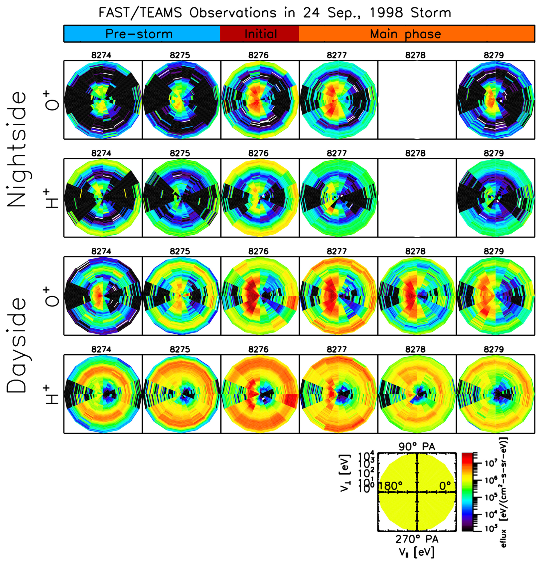
Figure 3 Energy–pitch angle plots of the outflowing number flux for the nightside aurora O⁺ (top row), the nightside aurora H⁺ (second row), the dayside cusp O⁺ (third row) and the dayside cusp H⁺ (fourth row), averaged over each outflowing time interval. It shows six consecutive orbits with two orbits (8274 and 8275) before the storm, one orbit (8276) on the initial phase and three orbits (8277–8279) on the main phase. Only the poleward segment of the nightside outflows is shown in this plot. Energy from 0.9 eV–12 keV is divided into 48 bins. Pitch angle, ranging from 0–360°, is divided into 16 pitch angle directions. The field line direction points to the right and the anti-field line direction points to the left, as shown by the right-bottom plot. The orbit number is labeled on the top of each panel. SSC occurs in orbit 8276. Panels for the nightside outflows in orbit 8278 are blank due to the data gap.

The top row shows the O⁺ distributions on the nightside. Before the storm, in orbits 8274 and 8275, as indicated by the blue mode bar, the outflow flux is comparatively low. The conic population becomes most intense just after the storm onset, orbits 8276 and 8277. Later in the main phase, the outflows become less intense and less energetic. The second row shows H⁺ on the nightside. The low-energy H⁺ ions also show the conic distributions. For the H⁺, the precipitating plasma sheet distribution is more continually present than for the O⁺. While there are clearly conics in orbits 8276 and 8277 after the storm commencement, they are not significantly more intense than some of the pre-storm orbits, such as the orbits 8265 and 8267 (not shown in Fig. 3) when the outflow flux is comparable to that of orbits 8276 and 8277. The third and fourth rows show the O⁺ and H⁺ distributions in the cusp. Overall, the cusp outflows are more intense than the nightside outflows. O⁺ shows a similar dependence on storm phases to the nightside. The flux is suddenly enhanced to its peak at the SSC to the level of ${\mathrm{10}}^{\mathrm{9}}\mathrm{ions}{\mathrm{cm}}^{-\mathrm{2}}{\mathrm{s}}^{-\mathrm{1}}$ and is intense during the main phase. The O⁺ flux is higher on the dayside than the nightside during the storm. The H⁺ outflow characteristics are similar, but less intense than O⁺. The precipitating population, from the magnetosheath, is much stronger for H⁺ than for O⁺.

3.3 Responses of the outflow to the energy input

The time history of the outflow flux and the energy input during the storm is shown in Fig. 4, with cusp on the left and nightside on the right. Panels (c) and (j) show both the O⁺ flux and the all-ion flux. The fluxes track very well indicating good cross-calibration between the two instruments. As was seen in Fig. 3, the cusp O⁺ flux (panel c) shows a clear strong increase in the initial phase, stays enhanced during the main phase, then returns to the level of the pre-storm times. The averaged intensity of O⁺ outflow in the nightside aurora (panel j) is generally weaker than the dayside cusp region (panel c). It also increases during the initial and early main phase, and then decreases. There is also a pre-storm increase in O⁺ in orbit 8265 and 8267, so the trend is less clear. The H⁺ ion outflow flux is shown in Fig. 4 (panels d and k). The cusp H⁺ has a clear peak during the initial phase and then decreases. As was clear in Fig. 3, the nightside H⁺ outflows are less affected by the conditions during storm times than the O⁺ outflows, with only a small increase, no larger than observed during some pre-storm periods.

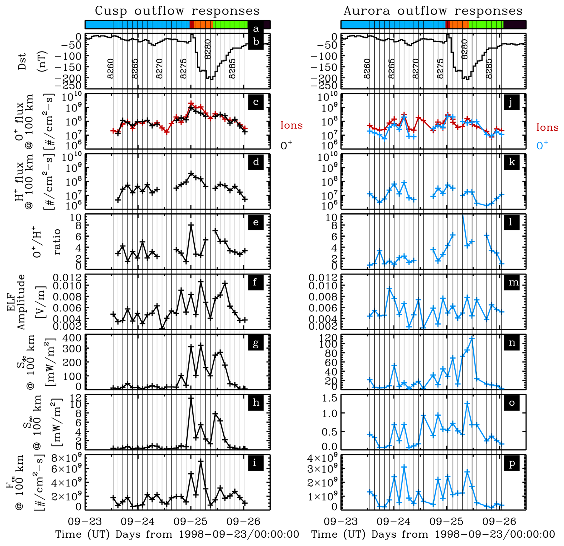
Figure 4 The evolution of the dayside cusp (left plot) and the nightside aurora (right plot) O⁺ and H⁺ outflows and the energy inputs during the storm. It shows (a) the storm phases (the color is the same as Fig. 1), (b) the Dst index, with some orbit numbers labeled, the averaged O⁺ outflowing number flux and the iESA outflow number flux, mapped to 100 km, over the dayside cusp region (c) and the nightside auroral oval zone (j), the averaged H⁺ outflowing number flux (d, k), the averaged ${\mathrm{O}}^{+}/{\mathrm{H}}^{+}$ flux ratio (e, j), and the averaged A_elf (f, m), the maximum S_dc (g, n), the maximum S_ac (h, o), and the averaged f_en in each dayside outflow segment and each poleward nightside outflow segment. The vertical reference line represents the start time of each outflow segment. There are 27 segments on the dayside since the orbit 8280 is excluded due to large fraction of missing data. There are 25 segments on the nightside as explained in Sect. 2.

The cusp energy input shows a very coherent storm-phase picture, with the ELF amplitude, S_ac and S_dc and f_en all increasing at storm onset. S_ac, reaches its maximum at the SSC while S_dc reaches its first peak value at the SSC, and both remain enhanced into the recovery phase. The wave activities and the precipitating electrons are most intense during the main phase. The nightside response is much less coherent. The nightside Poynting flux, S_dc, is enhanced during the storm time while the ELF wave activity, S_ac, and the electrons are variable throughout the magnetically quiet and active times, with no clear enhancement during the storm.

The ${\mathrm{O}}^{+}/{\mathrm{H}}^{+}$ flux ratio, panels (e) and (l) in Fig. 4, show a clear dependence on the storm phase. On the dayside, the ratio increases from a mean of 2.8 before the storm to 8.0 during the initial phase and ∼4.0 during the main and recovery phases. On the nightside, it starts lower, at 1.9 before the storm, increasing to 4.3 during the initial phase, 5.8 in the main phase, and 3.8 in the recovery phase. Thus, the storm increases the average ${\mathrm{O}}^{+}/{\mathrm{H}}^{+}$ flux ratio by a factor of 1.5 on the dayside and 2.5 on the nightside (ratio of storm-time average to quiet-time average). The ${\mathrm{O}}^{+}/{\mathrm{H}}^{+}$ changes more on the nightside than on the dayside during the storm mainly because of the small change in the H⁺ flux on the nightside, and because the ${\mathrm{O}}^{+}/{\mathrm{H}}^{+}$ ratio is higher before the storm on the dayside.

3.4 Solar wind controlling the energy input

To find the likely driving factors of the energy inputs, we test the correlation between the expected drivers of magnetospheric response, IMF B_z and solar wind dynamic pressure. In addition we test the solar wind-magnetosphere coupling function (Newell et al., 2007),

$${\displaystyle \frac{\mathrm{d}{\mathrm{\Phi }}_{\text{MP}}}{\mathrm{d}t}}=v^{\frac{\mathrm{4}}{\mathrm{3}}}{B}_{\mathrm{T}}^{\frac{\mathrm{2}}{\mathrm{3}}}{\sin }^{\mathrm{8}/\mathrm{3}}\left({\displaystyle \frac{{\mathit{\theta }}_{\mathrm{c}}}{\mathrm{2}}}\right),$$

which, as described in Sect. 2.1, estimates the rate of magnetic reconnection at the magnetopause. We use this function because Newell et al. (2007) found it a better parameter for representing the interaction between the solar wind and the magnetosphere than other coupling functions, including B_z, the solar wind dynamic pressure p, the half-wave rectifier vBs, and $\mathit{\epsilon }=v{B}_{\mathrm{T}}^{\mathrm{2}}{\sin }^{\mathrm{4}}({\mathit{\theta }}_{\mathrm{c}}/\mathrm{2})$. In addition, because we are examining the changes in the outflow during a storm, we also test the modified coupling function, $p^{\mathrm{1}/\mathrm{2}}\mathrm{d}{\mathrm{\Phi }}_{\text{MP}}/\mathrm{d}t$, which was found to have the best correlation with Dst. Because we are examining the effects of the large scale changes in the solar wind and IMF, we use a one-hour average of the solar wind and coupling parameters from one hour before the FAST outflow measurement. Tests of the correlations using simultaneous solar wind measurements and other smaller time intervals gave similar results, indicating that the large scale changes are dominating the correlation. For completeness, we also show the correlation between the outflow flux and the solar wind parameters, but we note that the connection between the solar wind input and the outflow flux is through the energy input.

Figure 5 shows the dependence of the three energy inputs and the outflow flux on the hourly average of the drivers. The correlation coefficients are listed in Table 1. The energy inputs show the strongest correlation with the coupling functions (panels c, d, g, and h). In the cusp region, S_dc and S_ac are well correlated to the coupling functions, $\mathrm{d}{\mathrm{\Phi }}_{\text{MP}}/\mathrm{d}t$, with correlation coefficients of 0.74±0.23 and $\mathrm{0.74}\pm \mathrm{0.23}.$ However, the correlation between f_en and the coupling function is weak. On the nightside, the correlations are weaker than the dayside with a coefficient of about 0.5.

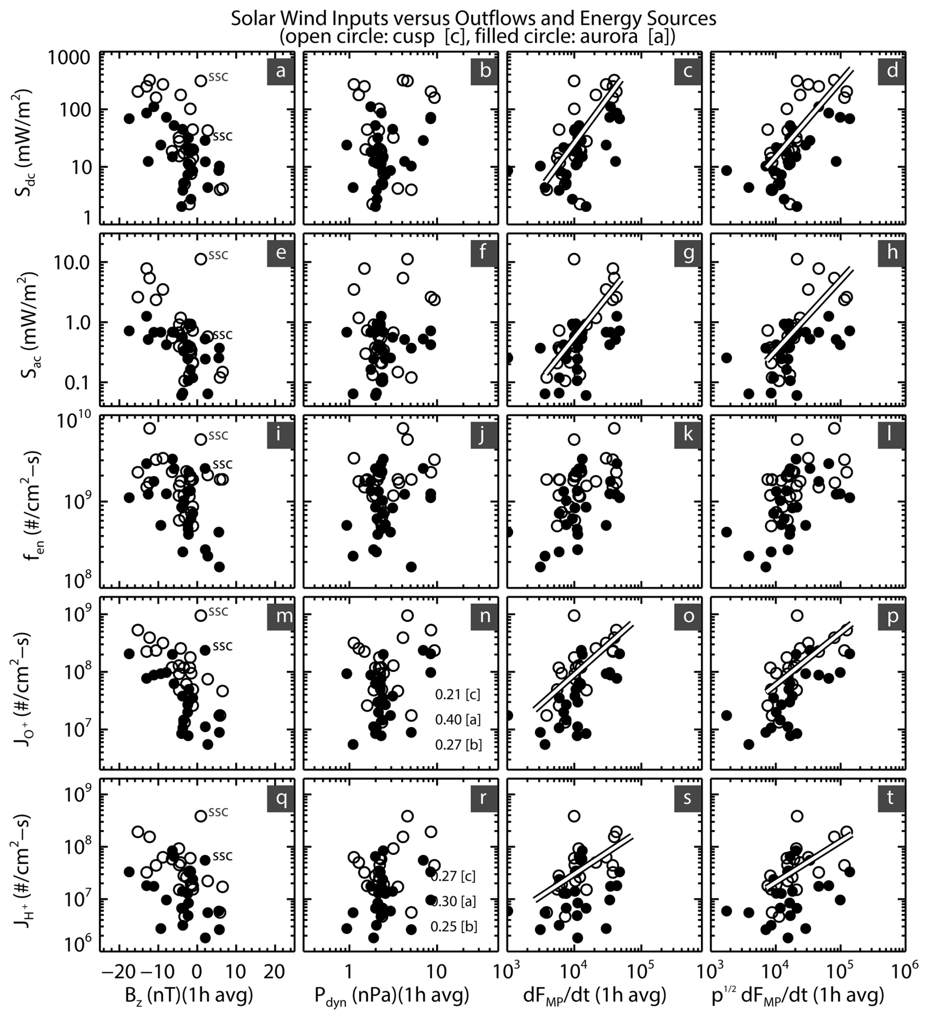
Figure 5 Scatter plots of the solar wind-magnetosphere coupling functions, B_z (leftmost column), P_dyn (second column from the left), $\mathrm{d}{\mathrm{\Phi }}_{\text{MP}}/\mathrm{d}t$ (third column from the left) and $p^{\mathrm{1}/\mathrm{2}}\mathrm{d}{\mathrm{\Phi }}_{\text{MP}}/\mathrm{d}t$ (rightmost column) versus the energy inputs, including S_dc, S_ac, and f_en , and the outflow fluxes, including $J_{{\mathrm{O}}^{+}}$ and $J_{{\mathrm{H}}^{+}}$. Intensities of the particle fluxes are averaged over the time period of the dayside cusp outflow (open circle) and the nightside aurora outflow (filled circle), while the maxima of S_dc and S_ac are used. The coupling functions are the averages over one hour prior the outflows observed by FAST. Correlations are computed for the dayside cusp, the nightside aurora, and the both regions, individually. In panels (c), (d), (g), (h), (o), (p), (s), (t), the best fitting lines are added to the scatters of the solar wind coupling functions, $\mathrm{d}{\mathrm{\Phi }}_{\text{MP}}/\mathrm{d}t$ and $p^{\mathrm{1}/\mathrm{2}}\mathrm{d}{\mathrm{\Phi }}_{\text{MP}}/\mathrm{d}t$ versus the energy inputs and the outflows in the cusp region.

Table 1 Correlation coefficients between the outflows, the energy inputs (rows) and the coupling functions (columns).

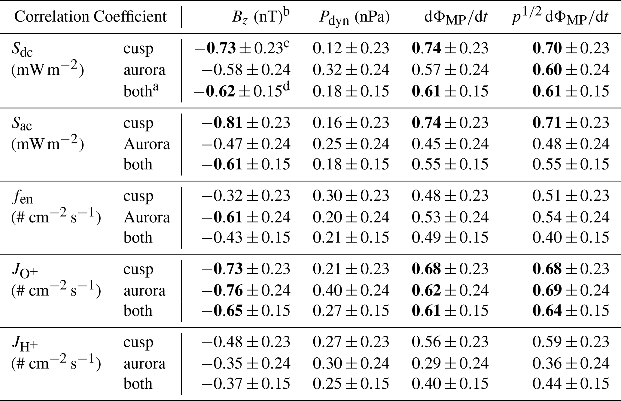
^a The data from both the cusp and the aurora are combined in this case. ^b The scatter in the initial phase is excluded in the correlation to B_z. ^c The uncertainty covers one standard deviation from the mean (approximately α≈0.30). ^d The absolute correlation coefficients above 0.60 are marked in bold.

The energy inputs show a clear negative trend with the IMF B_z, as shown in panels (a, e and i) in Fig. 5. However, because the average value of B_z is significantly positive during the period of SSC, as shown by the two labeled points when the FAST satellite passed the dayside and the nightside, we exclude the point of SSC when computing the correlation coefficients for B_z. It indicates that the energy inputs become enhanced when IMF turns southward and increase with decreasing B_z after the storm SSC. The intensity of the energy inputs does not show a significant correlation with the solar wind dynamic pressure, as shown in panels (b), (f), and (j) in Fig. 5.

As was shown in Zhao et al. (2020, 2022), the O⁺ outflow flux showed the most significant correlation with the DC and AC Poynting flux. Thus, we would expect the outflow to show correlations with the solar wind functions that are best correlated with the Poynting flux. The scatter plots of the orbital outflow flux versus the solar wind-magnetosphere coupling functions are shown in Fig. 5o, p, s and t. As expected, the result shows that the outflow flux scales with the coupling functions, $\mathrm{d}{\mathrm{\Phi }}_{\text{MP}}/\mathrm{d}t$ and $p^{\mathrm{1}/\mathrm{2}}\mathrm{d}{\mathrm{\Phi }}_{\text{MP}}/\mathrm{d}t$ which had the best correlation with the Poynting flux. As shown in Table 1, the correlation coefficients are $r(J_{{\mathrm{O}}^{+}},\mathrm{d}{\mathrm{\Phi }}_{\text{MP}}/\mathrm{d}t)=\mathrm{0.68}$, $r(J_{{\mathrm{O}}^{+}},p^{\mathrm{1}/\mathrm{2}}\mathrm{d}{\mathrm{\Phi }}_{\text{MP}}/\mathrm{d}t)=\mathrm{0.68}$ for the cusp O⁺ outflow and $r(J_{{\mathrm{O}}^{+}},\mathrm{d}{\mathrm{\Phi }}_{\text{MP}}/\mathrm{d}t)=\mathrm{0.62}$, $r(J_{{\mathrm{O}}^{+}},p^{\mathrm{1}/\mathrm{2}}\mathrm{d}{\mathrm{\Phi }}_{\text{MP}}/\mathrm{d}t)=\mathrm{0.69}$ for the nightside O⁺ outflow. Similar to the energy inputs, the outflow shows a negative correlation with IMF B_z and no significant correlation with the dynamic pressure.

The significant correlation between the energy sources and the coupling functions indicates that reconnection is the most significant cause of energy input into the auroral region. The lack of correlation with dynamic pressure emphasizes that it is not just the energy carried by the solar wind that is important, but the degree to which the energy is able to penetrate the magnetosphere.

4 Summary and conclusions

Nowrouzi et al. (2023) showed that the ionospheric outflow follows a clear pattern during a CME storm, increasing during the initial phase, remaining enhanced during the main phase, and then decreasing during the recovery phase. This study uses one event to track how the IMF and solar wind changes characteristic of a CME-driven storm drive this sequence. The leading edge of a classic CME has a fast forward shock, with increased plasma density and velocity that leads to the sharp dynamic pressure enhancement. The shock is often followed by a magnetic cloud that has a strong rotating field (Tsurutani and Gonzalez, 1997). When the magnetic field is southward, it drives the storm main phase. These characteristic signatures are clearly observed in this storm, as shown in Fig. 1, with a strong increase in the dynamic pressure and magnetic field magnitude during the initial phase, followed by the strongly southward B_z that coincides with the drop in Dst. The enhanced dynamic pressure and southward B_z both drive energy into the magnetosphere. Newell et al. (2007) tested multiple coupling functions to identify the parameters in the solar wind and IMF that most strongly drive the magnetosphere. The two best coupling functions are shown in the last two panels of Fig. 1. Clearly, the coupling increases strongly during the initial phase of the storm, remains high during the main phase and then decreases during the recovery phase. Figures 3 and 4 show that the outflow observed in this storm is consistent with the statistical picture shown in Nowrouzi et al. (2023), with strong outflow during the initial and main phase on both the dayside and nightside, but the strongest outflow on the dayside.

Figure 4 shows how the energy input into the auroral region measured in situ increases during the times when the coupling is strong. The dayside cusp shows a clear response to the changes in the solar wind, with both AC and DC Poynting fluxes as well as soft electron precipitation enhanced during the initial phase and main phase. On the nightside, the overall changes in the energy input are not as clear. The DC Poynting flux shows the clearest increase during the initial phase and main phase, while the AC Poynting flux and the electron precipitation variations with time do not show a strong consistent pattern. Figure 5 shows the correlation between the energy input into the cusp and nightside auroral regions and the driving parameters from the solar wind and IMF. Consistent with Fig. 4, the cusp Poynting flux input is well correlated with the coupling function. The dynamic pressure and B_z individually are not so well correlated, but the combination of parameters in the coupling function increases strongly during the storm initial and main phases and drives Poynting flux into the cusp region. The energy from precipitating electrons has a weaker correlation with the driving parameters. Correlations between the nightside energy input and the driving parameters are much weaker.

On the dayside, the sequence of events leading to enhanced outflow is clear. The changes in the solar wind due to the CME structure strongly drive the magnetosphere. This enhanced coupling at the magnetopause drives enhanced energy, particularly AC and DC Poynting flux, into the cusp region. This energy input then drives the enhanced outflow. The clear correlations observed on the dayside in this study are possible because during this storm the FAST orbit routinely passes through the localized region of strong energy input on the dayside. That the same clear chain is not observed as strongly on the nightside is likely due to two factors. First, there is some delay between the changes in the solar wind at the magnetopause and the effects on the nightside. The effects of enhanced dynamic pressure are observed almost without delay in the magnetosphere (Gamarra et al., 2020), but the response to a southward turning has some delay. The auroral electrojets respond to a southward turning with a delay of less than 5 min, and the tail-like deformation of the tail begins in ∼10 min (Sauvaud et al., 1987). But the onset of a substorm driven by the southward turning can take 40–80 min (Sauvaud et al., 1987; Samsonov et al., 2024), which is outside our 1 h averaging time. These delays will reduce the correlation between the averaged solar wind parameters and the energy input. The second factor is that the energy deposited on the nightside is spread over a larger, less continuous region. Thus, it is likely that one spacecraft measuring deposited energy in situ, will sometimes miss the energy input, even if it is significant. That the O⁺ outflow does show a clear flux increase on time scales similar to those observed on the dayside indicates that the outflow resulting from energy input may have a longer time duration than the energy input. The outflow would then show a steadier profile, even if the energy input is sporadic. A statistical study of the energy input using a large database of storms, similar to that done by Nowrouzi et al. (2023) for outflow, is needed to provide a better statistical estimate of the nightside energy input and response during a storm over a broader region to fully cover the auroral nightside energy input and output.

Following the progression of the energy input and the outflow in the auroral zone during a storm with satellite observations is difficult because of the long time scales of the storm compared to the time scales of a low altitude orbit. This storm was fortuitous in that the FAST satellite orbit was in the noon-midnight meridian, and so gave snapshots of the energy input and ion outflow in both the cusp and the nightside aurora every two hours during the course of the storm. This allowed the time series of the solar wind and IMF, the energy inputs to the dayside and nightside auroral regions, and the dayside and nightside ion outflow to be tracked for the first time during all phases of a single storm. This clearly showed that, while changes in individual solar wind and IMF parameters did not correlate well with the energy inputs to the aurora, the combined changes captured in the Newell et al. (2007) coupling functions do correlate with the changes in Poynting flux into the auroral regions. The changes in the Poynting flux drive the strong increases in the outflow observed during the storm.