Pre-earthquake Electric Field Disturbances and Interference Analysis Based on CSES-01 Satellite Observations

Anomalous electromagnetic phenomena in the ionosphere before seismic activity have been identified as potential indicators for earthquake early warning. Data from the CSES-01 satellite were analyzed using the STL decomposition method to break down electric field time series into longitudinal, latitudinal, and residual components. To quantify disturbance intensity, we use the C-value, a spectrum-fitting index derived from the power-law relationship between electric-field power spectral density and frequency. The longitudinal and latitudinal components reveal the electric field's double periodicity, characterized by a V-shape from south to north and a bimodal shape from east to west. After isolating conventional periodic disturbances with a strength of 0.87, unconventional disturbances in the residual component were examined to identify seismic precursor anomalies. Electric field power density disturbances associated with the 11 May 2023, Tonga Islands magnitude 7.6 earthquake were extracted. Multiple significant anomalies in the ionospheric electric field were detected within 20 d prior to the earthquake: an initial anomaly with a C-value exceeding 3.5 appeared 20 d before; a persistent anomaly with a peak C-value of 3.9 occurred 13 to 11 d prior; a sharp increase to a peak C-value of 4.4, three times the standard deviation, was observed 7 d prior; disturbances decreased until a resurgence 4 d prior, with a peak C-value of 3.5 lasting 2 d; the C-value returned to baseline 1 d before the earthquake. The STL-C method effectively differentiates various causal disturbances in the ionospheric electric field, offering novel approaches and insights for studying seismic precursors.

1 Introduction

The ionosphere, as part of the upper atmosphere, plays a crucial role in the Earth's atmospheric system. Situated at an altitude of approximately 60 to 1000 km above the Earth's surface, this layer is characterized by a high degree of ionization, containing numerous ions and free electrons. Its uniqueness lies in its ability to reflect radio and other electromagnetic waves, fundamentally impacting global communication systems and radar detection technologies. The ionosphere's state is influenced by various external factors, including geomagnetic effects, solar activity, diurnal and seasonal variations, and natural phenomena such as magnetic storms and earthquakes. Diurnal variations in the ionosphere primarily manifest as differences in ionization levels between daytime and nighttime, caused by the increased solar radiation during the day. Seasonal variations relate to changes in the Earth's orbital position, affecting the angle and duration of solar radiation incidence. Although solar activity is considered the primary source of ionospheric variability in ionospheric physics, recent studies have established that significant effects on the ionosphere, such as those from volcanic eruptions and magnetic storms are substantial (Sokolov, 2011; Pulinets et al., 2022). Strong earthquakes are also recognized as important perturbation sources, as documented in numerous publications (Silina et al., 2001; Astafyeva et al., 2013). During the preparation and occurrence of earthquakes, the ionosphere in and around the source region exhibits varying degrees of electromagnetic phenomena, typically appearing days or hours before the onset of an earthquake, making them potential precursor indicators (Sarkar et al., 2007).

Since the 1960s, the phenomenon of pre-seismic ionospheric disturbances has garnered extensive attention from scientists (Astafyeva, 2019). As early as 28 March 1964, following the Alaska earthquake, Leonard and Barnes (1965) observed two forms of ionospheric disturbances at four ionospheric stations and found that the disturbances' nature depended on the distance between the observatory and the earthquake's epicenter. In the same year, Davies and Baker (1965) observed irregular disturbances in various high-frequency bands (10, 5, and 4 MHz) before and after the main shock. This discovery sparked significant interest among scientists in detecting earthquakes within the near-Earth spatial range, leading to studies exploring the relationship between earthquakes and ionospheric variations using both ground-based and space-based observations. Using data from the Sugadaira Space Radio Observatory (SRO) in Japan, Silina et al. (2001) recorded electromagnetic signals with amplitudes 15 dB higher than usual prior to the mainshock. Similarly, Larkina et al. (1983), using data from Intercosmos 19, found an unusual increase in VLF signal strength in the F-region of the ionosphere both before and hours after the earthquake. Parrot and Mogilevsky (1989), using data from the geosynchronous satellite GEOS 2 and the polar satellite Aureol 3, discovered a significant increase in VLF signal strength in the F-region of the ionosphere. They also found that earthquakes can cause electromagnetic disturbances in the ionosphere, manifesting as electromagnetic wave disturbances and electron density enhancements in the Es layer. Chmyrev et al. (1989), using data from the Intercosmos Bulgaria 1300 satellite, studied an earthquake on 21 January 1982, and found significant electrostatic and magnetic field disturbances over the epicenter within the first ten minutes. Serebryakova et al. (1992) studied ELF electromagnetic radiation detected by the low-orbiting satellites COSMOS 1809 and AUREOL-3 as they passed over the seismic region. They found strong electromagnetic radiation in the frequency band below 450 Hz in the magnetic crust parameters corresponding to the earthquake's epicenter, persisting throughout the region of seismic activity. Together, these pioneering works laid the foundation for studying earthquake-related ionospheric disturbances; however, investigations into how various external factors may interfere with the observed electromagnetic signals remain relatively limited.

Since then, numerous studies have focused on seismic ionospheric disturbances, with scholars deepening their understanding of the seismic ionosphere's response mechanisms through various observational means and data analysis methods. As short-term precursors to earthquakes, seismic electromagnetic phenomena primarily manifest within days to hours before seismic events. Bhattacharya et al. (2007) found that Ultra Low Frequency (ULF), Extremely Low Frequency (ELF), and Very Low Frequency (VLF) electromagnetic waves, due to their greater penetration depth and reduced attenuation, are observed more prominently during seismic events. Since the 20th century, both ground-based and satellite observations have demonstrated that a broad spectrum of electromagnetic (EM) signals can be detected in the vicinity of major earthquakes (Pulinets, 2004). These EM disturbances persist for a longer duration on the ground, whereas they are consistently observed in space within days or even hours before an earthquake (Shen et al., 2018).

On 2 February 2018, China's first space-based platform for three-dimensional earthquake observation, the pilot satellite of the National Geophysical Field Exploration Satellite Project, CSES-01, was successfully launched, playing a significant role in global space environment monitoring. The satellite's primary mission is to construct a space-based experimental platform for monitoring key physical quantities, such as global electromagnetic fields, electromagnetic waves, ionospheric ions, and energetic particles (Zhima et al., 2022; Martucci et al., 2022). This enables quasi-real-time monitoring and tracking of China and its neighboring regions, as well as research on electromagnetic information for earthquakes of magnitude 7 or above globally and magnitude 6 or above in China (Marchetti et al., 2020; Li et al., 2022). Additionally, it aims to explore the characteristics and mechanisms of ionospheric response to earthquakes (Chen et al., 2023). In this study, night-side electric field data collected by the CSES-01 satellite before and after the 7.6 magnitude earthquake in the Tonga Islands on 11 May 2023, are analyzed. Using a time series decomposition algorithm, cyclic disturbances affecting the observed ionospheric effects in the longitudinal and latitudinal directions are identified and removed. Further analysis is conducted on the residuals, accurately extracting the anomalous disturbance characteristics of the earthquake's precursor electric field, proving the method's effectiveness.

2 Data and Methods

2.1 Study Area and Data Selection

A strong earthquake, with a magnitude of 7.6, struck the Tonga Islands (15.50° S, 174.50° W) on 11 May 2023, at 00:02 Beijing Standard Time (BST; 16:02 UTC on 10 May 2023) and occurred at a depth of 200 km. According to the empirical formula for the lithospheric seismogenic zone proposed by Dobrovolsky et al. (1979):

$$\begin{array}{}\text{(1)}& R={\mathrm{10}}^{\mathrm{0.43}M},\end{array}$$

in which “M” represents the earthquake magnitude and “R” represents the radius of the seismogenic zone in kilometers, the radius of the seismogenic zone for the Tonga Islands earthquake is determined to exceed 1850 km. Consequently, the study area has been defined to encompass a region extending ± 20° from the earthquake's epicenter.

In this study, electric field data in the ELF band (19.5–250 Hz) observed by the CSES-01 satellite were utilized. The orbital revisit period of CSES-01 is approximately 5 d. The onboard Electric Field Detector (EFD) can measure electric fields in the ULF, ELF, VLF, and HF bands, providing three-component time-series data as well as Power Spectral Density (PSD) data. The ELF data are recorded with 1024 frequency bins covering 6 Hz–2.2 kHz, with a frequency resolution of 0.225 Hz. For the ELF analysis, the x-component of the electric field PSD was selected.

To date, the CSES-01 satellite has generated one of the most comprehensive datasets in the field of ionospheric electric field observations. The CSES-01 satellite and its payload, both in good operating condition, have demonstrated strong performance in monitoring natural phenomena such as magnetic storms and seismic activity. Research has confirmed the high reliability of the satellite observations, yielding significant results, particularly in the validation of electric field data (Huang et al., 2023a). These results have provided robust data support for scientific research and disaster prevention. In this study, observations from the night-side of the satellite were primarily utilized to enhance data quality. Night-time data exhibit smaller daily amplitude variations and are more sensitive to sudden ionospheric disturbances.

2.2 Research Methodology

2.2.1 STL decomposition

STL (Seasonal and Trend Decomposition using Loess) is a versatile and robust method for time series analysis. Developed by Cleveland et al. (1990), this method is based on Loess (Locally Weighted Scatterplot Smoothing). It is not only fast to compute but also maintains its efficiency even for very long time series with extensive trend and seasonal smoothing. STL decomposes a time series into seasonal, trend, and residual components. The seasonal component captures regular, repeating patterns, the trend component indicates the underlying direction of the data, and the residual component represents irregular fluctuations. Recent studies have demonstrated the usefulness of STL in geophysical satellite applications, such as GNSS-based tropospheric and ionospheric time-series analysis during volcanic eruptions (Barba et al., 2023) and MODIS sea surface temperature reanalysis (Jonasson et al., 2023).

In a mathematical formulation, the data in a time series can be represented by the following Eq. (2):

$$\begin{array}{}\text{(2)}& y_{\mathrm{t}}=S_{\mathrm{t}}+T_{\mathrm{t}}+R_{\mathrm{t}},\end{array}$$

Where y_t is the data, S_t is the seasonal component, T_t is the trend component, and R_t is the residual component.

The design of the STL decomposition allows flexible control of the seasonal and trend components, offering advantages such as robustness to outliers and adaptability to different temporal scales. Firstly, it allows control over the rate of change of seasonality and the smoothness of the trend period – including monotonic seasonality – which enables optimal tailoring of the specificity of the time series being analyzed. Secondly, STL exhibits robustness to outliers. Even in the presence of missing values and outliers, these anomalies do not affect the estimation of the trend cycle and seasonal components(Sohrabbeig et al., 2023). Consequently, these properties render STL particularly suitable for analyzing satellite data with large volumes. In this study, STL decomposition was implemented using a seasonal window of 7 and a period of 5200, applied to the transformed electric field time series. These settings were chosen to capture the dominant orbital-scale periodicity while suppressing short-term fluctuations.

2.2.2 Intensity Calculation

STL decomposition, as a method of analyzing time-series data, can clearly identify the intensity of seasonal and trend changes. Based on the results of STL decomposition, the seasonal intensity F_S can be calculated using:

$$\begin{array}{}\text{(3)}& F_{\mathrm{S}}=\text{max}\left(\mathrm{0},\mathrm{1}-{\displaystyle \frac{\text{Var}\left(R_{\mathrm{t}}\right)}{\text{Var}(S_{\mathrm{t}}+R_{\mathrm{t}})}}\right)\end{array}$$

Where F_S denotes the intensity of the seasonal component, Var(⋅) denotes variance, declaring R_t as the residual component and S_t as the seasonal component. Var(R_t) is the variance of the residual, and Var(S_t+R_t) is the variance of the seasonal-plus- residual component.

Similarly, the trend strength F_T can be calculated as follows:

$$\begin{array}{}\text{(4)}& F_{\mathrm{T}}=\text{max}\left(\mathrm{0},\mathrm{1}-{\displaystyle \frac{\mathrm{Var}\left(R_{\mathrm{t}}\right)}{\text{Var}(T_{\mathrm{t}}+R_{\mathrm{t}})}}\right)\end{array}$$

Where F_T denotes the intensity of the trend component. Var(R_t) is the variance of the residual, and Var(T_t+R_t) is the variance of the trend-plus-residual component.

F_S(F_T) takes values from 0 to 1, with 0 representing the absence of seasonality (trend) in the time series, and values close to 1 indicating a significant seasonal (trend) component. F_S and F_T therefore not only provide mathematical measures of seasonality and trend, but also have clear physical meaning in the context of ionospheric electric field analysis. A higher F_S value implies that the observed fluctuations are largely governed by regular periodic variations, whereas a lower F_S indicates that irregular or non-seasonal processes dominate. Similarly, a higher F_T reflects a persistent underlying trend in the data, while a lower F_T indicates the absence of systematic drift. These indices allow us to quantitatively evaluate the relative contribution of conventional periodic and trend-like processes, providing a reference baseline for identifying anomalous disturbances in the residual component.

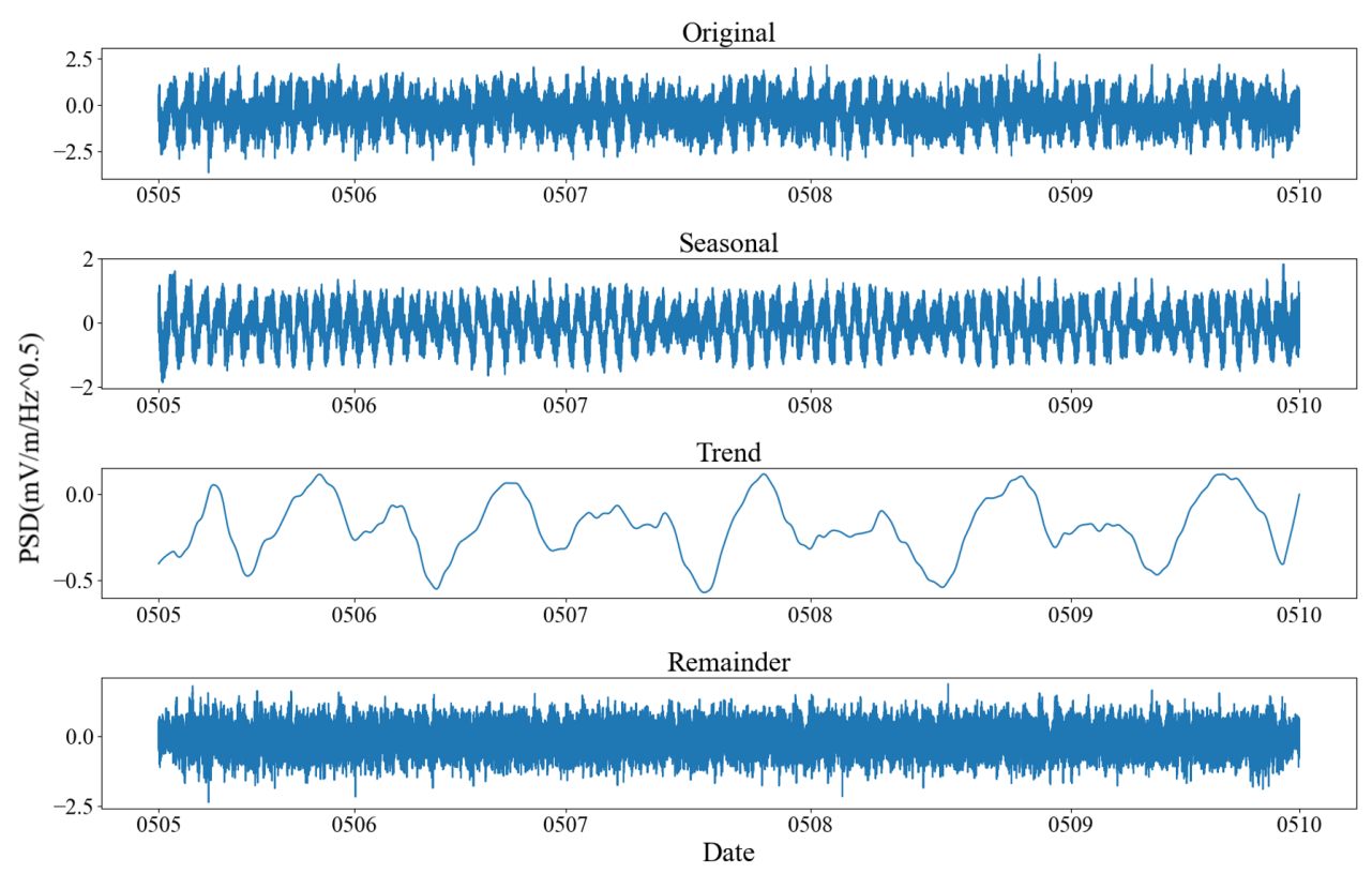
Figure 1 STL decomposition results for 6–10 May. From top to bottom: original PSD series after amplification and logarithmic transformation; seasonal (periodic) component; long-term trend; and remainder (residual) after removing the seasonal and trend components.

2.2.3 C-value

In previous studies, electromagnetic signals have been shown to exhibit fractal features in some ground-based ULF magnetic field data processing. Based on this, Zhang et al. (2010) proposed a method for identifying low-frequency electric field perturbations, defining an exponential relationship between the spectral data S_E and the frequency f using Eq. (5). In this study, the fitting is applied to the ELF band within 19.5–250 Hz. The following Eq. (5) is used to identify low-frequency electric field perturbations:

$$\begin{array}{}\text{(5)}& S_{\mathrm{E}}=a\cdot f^{-b},\end{array}$$

Further, Eq. (6) is constructed by logarithmically converting Eq. (5) and taking the absolute value, defining the function C:

$$\begin{array}{}\text{(6)}& C=a_{\mathrm{0}}+b\times \left|R\right|,\end{array}$$

Where a₀=loga. In applying this method, the parameters a, b, and the correlation coefficient R are extracted by fitting the spectral data S_E to the frequency f, and the value of C is calculated based on the result. The interpretation of the C-value is relative to a quiet-time baseline: values close to the baseline indicate ordinary background variations, whereas elevated values above the baseline suggest enhanced disturbances that may be associated with anomalous ionospheric activity. The C-value is used in this study to measure the perturbation of the electric field power density (Huang et al., 2023b).

3 Experimental Results

3.1 Satellite Data Analysis

STL decomposition, a method widely used for time series analysis, decomposes time series data into three components: seasonal, trend, and residual. The primary distinction between this study and prior applications of this method is the shift from predictive analyses to residual-based analysis of anomalous pre-seismic electric field perturbations. This approach reduces conventional perturbations, thereby revealing or emphasizing unconventional perturbations associated with earthquakes. Additionally, utilizing the isolated seasonal and trend components enables the study of conventional perturbations that affect observed ionospheric effects and their underlying physical causes. Figure 1 illustrates the STL decomposition results for the five-day revisit cycle that precedes the earthquake.

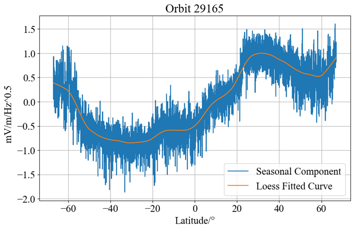
Figure 2 Latitudinal profile of the seasonal component for orbit 29165. (The orange line shows the Loess fit to the seasonal data).

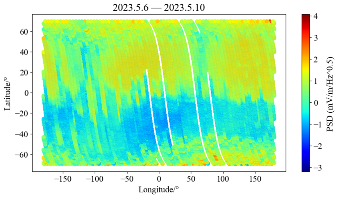
Figure 3 Spatial distribution map of the Original PSD data observed by CSES-01 from 6 to 10 May 2023.

The Original subplot in Fig. 1 presents the results of the original data after amplification and logarithmic processing, revealing distinct dual-periodic fluctuations in the PSD. The Seasonal subplot illustrates the data's periodic trend, depicting periodic changes in the longitudinal direction of the electric field. In the seasonal component, a stable cyclical trend that decreases and then increases within a single orbit forms a V-shaped trend. The Trend subplot depicts the long-term trend of the data, corresponding to variations between satellite orbits and representing periodic variations in the latitudinal component of the electric field. This subplot distinctly shows a dual-peak trend with clear daily periodicity. The Remainder subplot displays the raw PSD, subtracting the seasonal and trend components, and reveals the residual data that clearly retains the anomalous features suggested by the data.

3.2 Analysis of Influencing Factors

Among the three components decomposed by STL, the seasonal and trend components both exhibit distinct periodicity. The origin of this periodicity is primarily linked to the orbital cycle of the satellite and geographic variation in the ionospheric environment. Since the satellite orbits the Earth 15 times per day, the repeat cycle of ascending and descending passes produces orbit-related periodic signatures. In addition, longitudinal differences in ionospheric electrodynamics, such as lightning activity and current systems, contribute to the observed spatially dependent periodic fluctuations.

Specifically, the seasonal component follows a single satellite orbit as a cycle, revealing variations in the electric field from 65° S to 65° N latitude. As shown in Fig. 2, the seasonal component, decomposed from the night-side ascending orbit 29165, corresponds to the first V-shaped trend of the seasonal component in Fig. 1 and is associated with an orbit within the 0–50° E range in the orbital projection of the PSD in Fig. 3. From the trend fitted by Loess, the value of the component decreases from 65° S, enters a trough at about 40° S, rises near the equator, reaches a peak at about 30° N, then decreases slightly, and rises again. The spatial distribution of the PSD in Fig. 3 corroborates this.

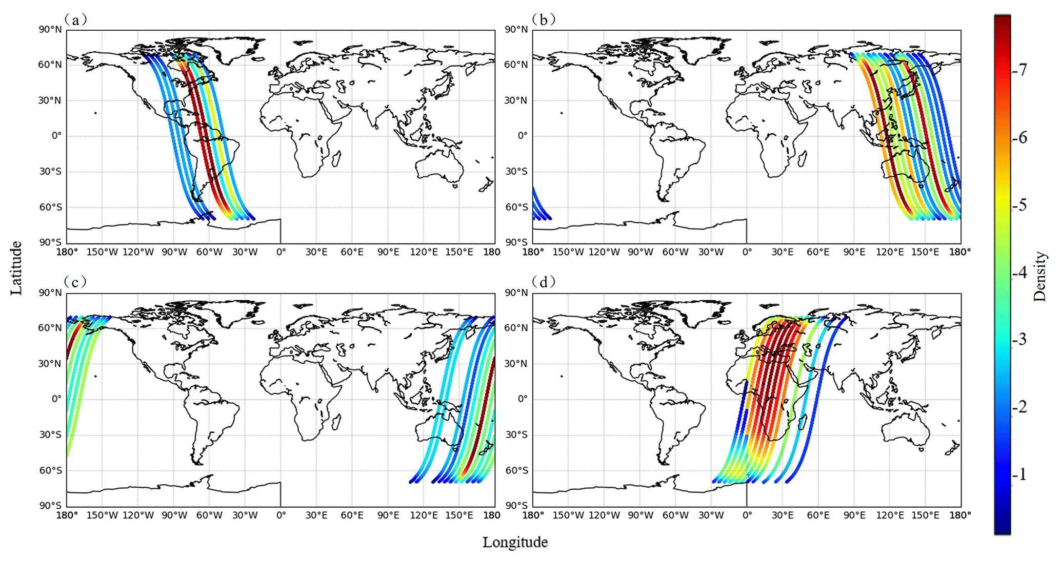
Figure 4 Spatial density distribution of the trend component peaks observed during May 2023. The colorbar indicates the density of peak occurrences (Unit: Counts). The subplots show the distributions for: (a) the first peak of the ascending orbits; (b) the second peak of the ascending orbits; (c) the first peak of the descending orbits; and (d) the second peak of the descending orbits.

The seasonal intensity is determined to be 0.67 according to Eq. (3), which indicates that the seasonal component comprises a larger proportion of the overall time series perturbations. Specifically, the perturbation of the longitude term explains 67 % of the total perturbations in the data. This high contribution reflects the systematic variation of the electric field with latitude along each orbital pass, as the satellite samples from high latitudes through the equatorial region. The perturbations observed in the high latitude and equatorial regions are likely due to the ionospheric electric field being significantly influenced by interactions between the polar region's auroral current and magnetic field, and by the equatorial current band(Weimer, 1995; Forbes, 1981).

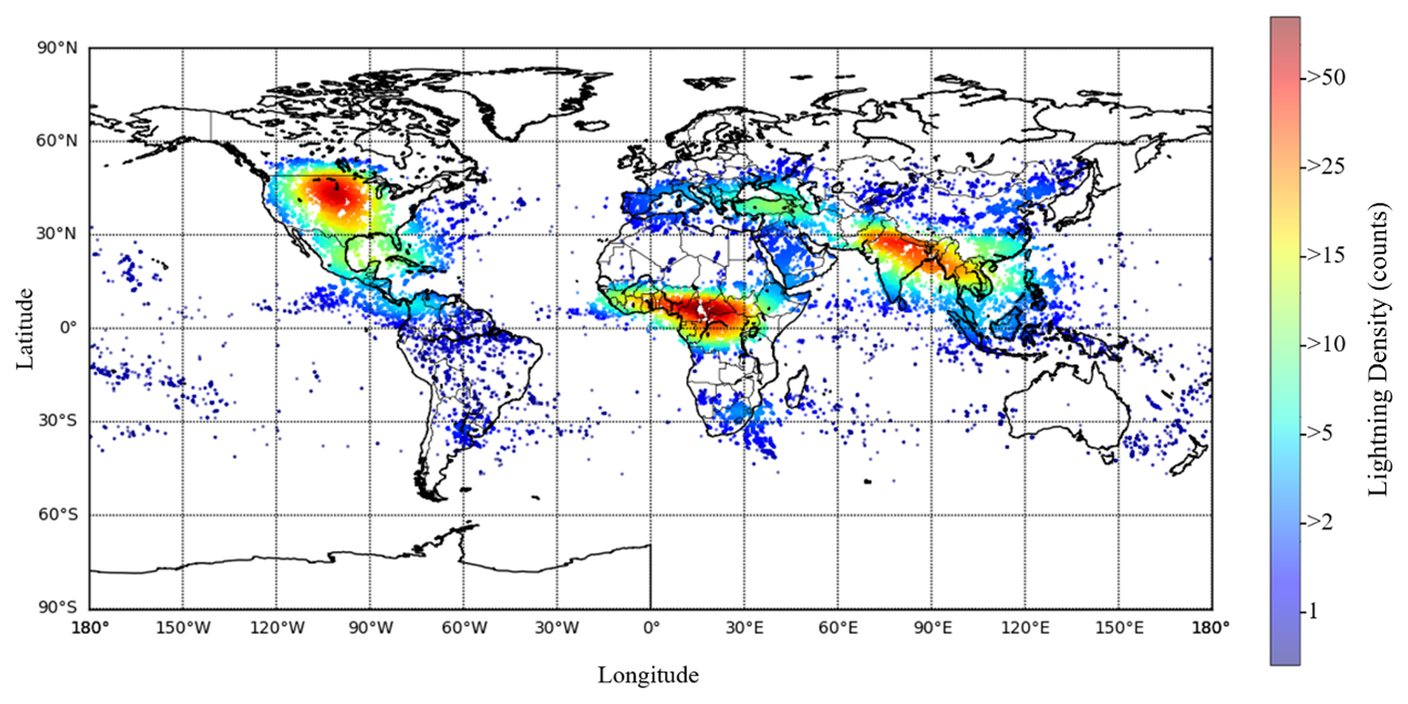
Figure 5 Global distribution of lightning activity in May 2023, based on data from the Lightning Imaging Sensor (LIS).

Given that the satellite orbits the Earth 15 times in a single day, with its orbital position continuously shifting westward, the latitudinal spacing between adjacent ascending or descending orbits is approximately 24°, resulting in a total daily shift of approximately 360°. Consequently, the dual-peak cyclic fluctuations in the trend component, observed daily, reflect variations between successive orbits and meridional changes in the ionospheric electric field from east to west. The bimodal peak regions in the daily ascending and descending orbits in May are statistically summarized in Fig. 4, which presents the density distribution of the peak-orbit data. Figure 4a and b display the spatial density distribution of the first and second peaks of the ascending orbits, respectively; Fig. 4c and d display the spatial density distribution of the first and second peaks of the descending orbits. The first peak of the ascending orbit is distributed over the American continent, with the highest data density near 60° W, indicating frequent peak occurrences at this location. The spatial distribution of the second peak of the ascending orbit is wider, spanning the eastern regions of Asia and Australia, as well as the western region of the Pacific Ocean, with two high-frequency peak areas near 110 and 160° E. The first peak of the descending orbit is located in the Pacific region, with a high-frequency peak area near 170° E. The second peak of the descending orbit is primarily located in Europe and Africa, with a wide range of high-frequency peak areas from 0 to 30° E. In addition, the spatial distribution of the peaks in the four subplots transitions from edge areas with lower frequency to high-frequency peak areas and then back to edge areas. The relationship between distribution frequency and longitude approximates a normal distribution. The peak distribution area shows a high degree of overlap with the lightning aggregation areas. To facilitate a direct comparison, the trend component peaks in Fig. 4 were statistically summarized for the entire month of May 2023, ensuring a one-to-one correspondence with the global distribution of lightning in May 2023, as illustrated in Fig. 5.

The calculated intensity of the trend component from Eq. (4) is 0.20, indicating that approximately 20 % of the total variance is attributed to long-term systematic variations. Although this proportion is smaller than that of the seasonal component, the trend still captures physically meaningful background fluctuations in the ionospheric electric field. Given that lightning-dense regions can affect the F layer – where the satellite measurements are made – through mechanisms such as electromagnetic pulses, atmospheric electric field perturbations, gravity waves, and ionochemical reactions, it is hypothesized that the peak of the disturbance in the trend component may be influenced by high-density lightning activity.

The sum of the seasonal and trend strengths is 0.87, indicating that a majority of the time series fluctuations are decomposed into periodic regular perturbations. Furthermore, this suggests that the STL decomposition algorithm possesses significant explanatory power for the satellite data. The residuals mainly capture random noise and anomalous disturbances, which comprise only a minor portion of the data. These perturbations become more pronounced upon removal of the significant periodic components associated with latitude and longitude coordinates. By eliminating prevalent disturbances in the ionospheric electric field, the residuals now more closely align with the assumption of randomness. Consequently, when anomaly detection algorithms are applied to the residual data, enhanced performance is anticipated.

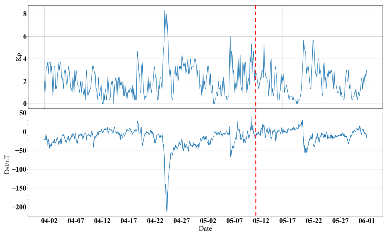
Figure 6 Variations in Kp and Dst indices from 1 April to 31 May 2023 (Red Dashed Line Indicates the Time of Earthquake Occurrence).

3.3 Case Study of Earthquakes

At satellite altitudes, the electromagnetic field, in addition to exhibiting background variations from regular solar activity (such as diurnal and seasonal changes), is also significantly affected by geomagnetic activity, earthquakes, and solar eclipses. Prior to extracting information about anomalous perturbations associated with seismic precursors, it is essential to consider and eliminate these spatial perturbation factors within the studied time period. For this study, geomagnetic activity is assessed using the Dst and Kp indices. The effects of the Kp and Dst indices on magnetic storm activity both before and after the earthquake are illustrated in Fig. 6. The results indicate that strong magnetic storms – characterized by a Dst value less than −200 and a Kp greater than 8 – occurred on 23–24 April, while moderate magnetic storms – with a Dst value less than −50 and a Kp greater than 4 – occurred on 6 and 20 May. Furthermore, no solar eclipses or artificial transmission signals were present in the study period and region. Therefore, any ionospheric anomalies identified after excluding these known disturbances can be considered signals of this earthquake's precursor.

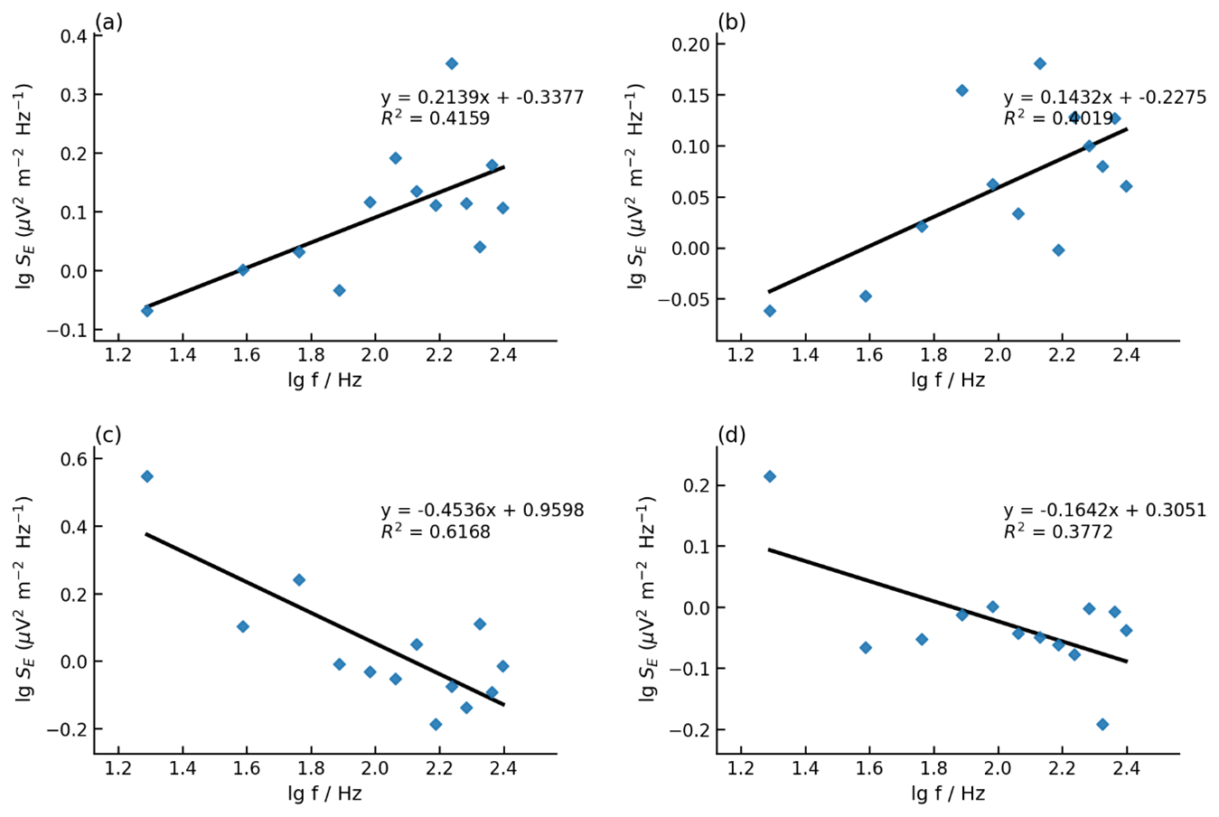
Figure 7 Linear fitting at four randomly selected observation points within one orbital cycle. (Each panel displays the logarithm of the electric field spectrum (blue diamonds) as a function of the logarithm of the frequency. The black line indicates the regression fit, with the corresponding equation and coefficient of determination (R²) shown in the top right corner of each panel).

To analyze the unconventional perturbation information embedded in the power density residuals and to extract electric field perturbation features associated with earthquakes, an STL decomposition of the PSD values across multiple frequencies is initially performed to obtain the PSD residuals for each frequency. Subsequently, the residual values and frequencies are fitted to the parameters a and b, and correlation coefficients R, as delineated in Eq. (5). Finally, the STL-C values are calculated as per Eq. (6). Representative examples of the spectral fitting and regression are shown in Fig. 7.

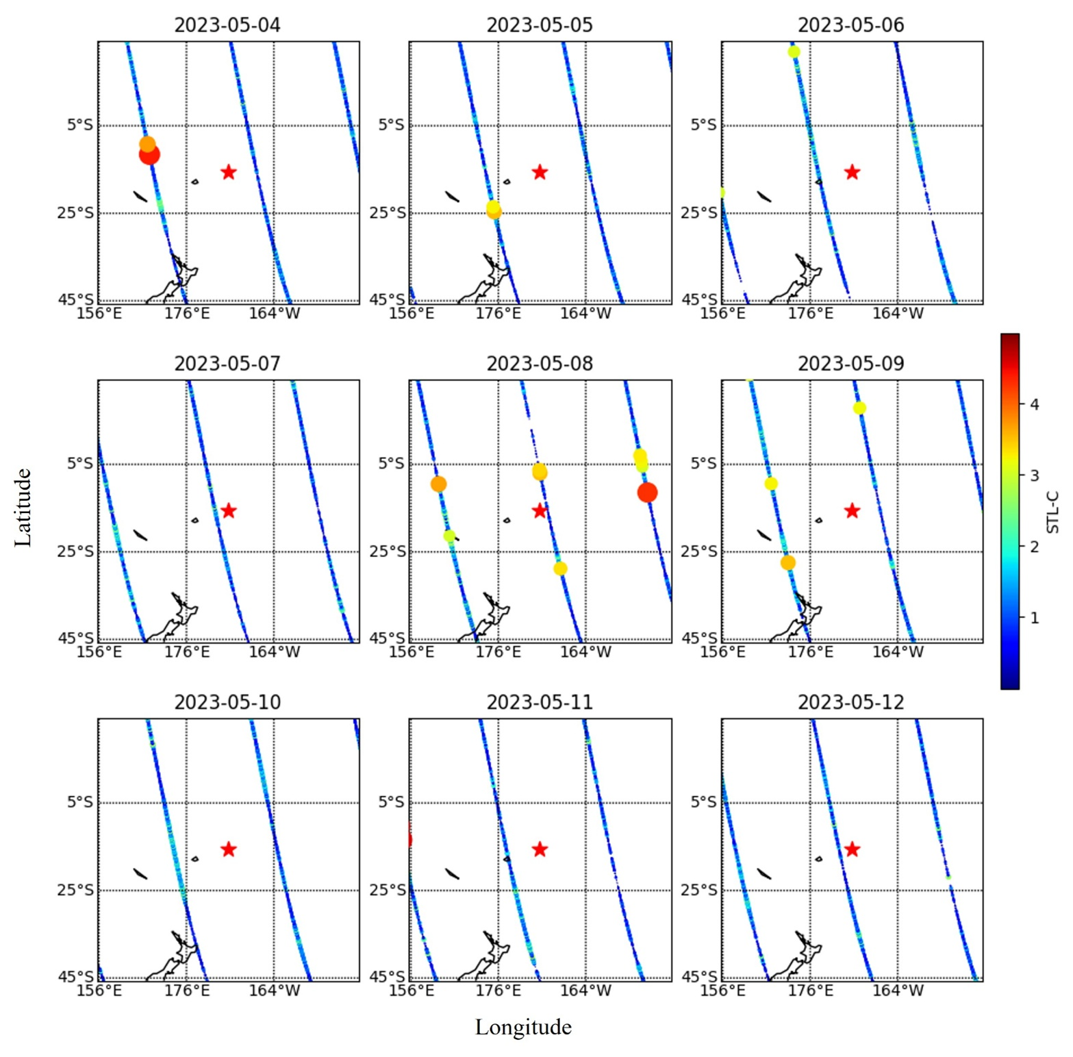
Figure 8 Daily variations of anomalous STL-C values surrounding the M_w  7.6 Tonga earthquake epicenter (red star) from 4 to 12 May 2023. The colored dots represent these anomalous STL-C values along the satellite ground track; both the size and color of the dots are scaled to their magnitude. The colorbar indicates this magnitude (Unit: unitless).

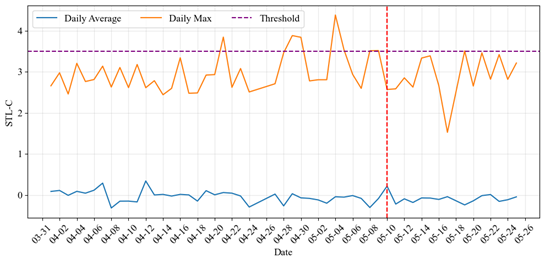
Figure 9 Variation Characteristics of STL-C Maximum and Average Values from 1 April to 26 May 2023. (Red Dashed Line Indicates the Time of Earthquake Occurrence).

For spatial visualization of the anomalies, the satellite data were mapped within a ± 30° latitude/longitude window centered on the epicenter. The data were gridded and plotted using a cylindrical projection with 20° meridian and parallel intervals. Color scales were normalized to the full data range for each event, and marker sizes were scaled with the magnitude of the STL-C values. This approach ensures that spatial resolution is sufficient to capture regional anomaly patterns while maintaining comparability across different orbits. To clearly illustrate the spatial evolution of the anomalies as a case example, Fig. 8 is presented in a nine-panel format covering 7 d before and 1 d after the event (the temporal evolution over a longer period is detailed in Fig. 9).

Electric field power spectrum data collected by the CSES-01 satellite before and after the M_w  7.6 earthquake in the Tonga Islands on 11 May 2023, were processed and analyzed. The period spanning 7 d before to 1 d after the earthquake (4–12 May 2023) was selected for the study. As illustrated in Fig. 8, on 4 May, the C-value exhibited an anomaly in the northwestern region of the seismogenic zone, reaching a peak of 4.4. On 5 May, the C-value in the southwestern region declined slightly to 3.5. On 6 and 7 May, the highest C-value further decreased to 2.5, indicative of a low-level state. On 8 and 9 May, anomalies were observed in various directions near the center of the seismogenic zone, with the highest C-value rising above 3.5. On 10 May the day before the earthquake, the C-value dropped to 2.5. No significant changes were observed on the day of the earthquake or in the days following, indicating a return to baseline levels. This pattern suggests an anomalous increase in the C-value prior to the earthquake, indicating a discernible trend in the extreme values.

Figure 9 depicts the temporal variation characteristics of the C-value maxima in the seismogenic zone from 40 d before the earthquake to 15 d after the earthquake. The anomalous disturbance, characterized by a C-value greater than 3.5, first appeared on 21 April (20 d before the earthquake) and was of short duration. The disturbance re-emerged from 28 to 30 April (13–11 d before the earthquake), lasting 3 d, with the C-value maxima reaching 3.9 and a disturbance amplitude approximately two times the standard deviation. On 4 May (7 d before the earthquake), the maximum C-value rose to 4.4, the highest value in the two months before and after the earthquake, with a perturbation amplitude approximately three times the standard deviation. The perturbation amplitude then declined from 5 to 7 May (6–4 d before the earthquake), rebounded on 8 May (3 d before the earthquake) with a maximum C-value of 3.5 for 2 d, and stabilized at a relatively low level on 10 May (1 d before the earthquake). After the earthquake on 11 May, the electric field remained stable.

4 Discussion and Conclusion

4.1 Discussion

In this study, we utilize the latitude and longitude components decomposed by STL to investigate the periodic disturbances impacting the ionospheric effects observed in satellite data. Additionally, we analyze the ionospheric effects before and after earthquakes using residual data obtained by removing these disturbances. Excluding the effect of conventional disturbances in the ionospheric electric field can make the information about earthquake precursor anomalies in the data more apparent. This exclusion also enables unconventional anomalous disturbances to emerge more prominently over the timescale of several weeks, as supported by the detection of multiple anomalies within the 20 d preceding the M_w  7.6 Tonga Islands earthquake. The spatial and temporal distributions of these anomalous disturbances display a distinct pattern.

Before discussing possible physical implications, we emphasize that the STL-based components and the derived metrics provide primarily a descriptive partition of the observations into periodic variations and residual disturbances. At this stage, the physical interpretations of the extracted patterns should be regarded as tentative and require further validation. The seasonal and trend components of the STL decomposition of the electric field data, respectively reflect the longitudinal and latitudinal variations of the ionospheric electric field. These components reveal a V-shaped periodic trend from south to north and periodic bimodal fluctuations from east to west in the satellite observation data. The seasonal component, which has a period corresponding to a single satellite orbit, is markedly influenced by latitudinal effects. In high-latitude regions, interactions with auroral currents and the magnetic field substantially influence the ionospheric electric field. In equatorial regions, factors including the equatorial electrojet among others, contribute to the seasonal component, thereby influencing the ionospheric electric field. The cyclic bimodal fluctuations of the trend component daily reflect changes in the electric field's latitudinal direction from orbit to orbit. A comparison of the bimodal peak distribution with global lightning distribution indicates a significant overlap between regions of high-density lightning and the distribution of the trend wave. This suggests that lightning can influence the ionospheric F-layer through mechanisms such as electromagnetic pulses, changes in the atmospheric electric field, gravity waves, and ionochemical reactions, resulting in partial perturbations of the peaks of the trend component wave.

The calculated seasonal strength of 0.67 and trend strength of 0.20 suggest that 87 % of the data fluctuations in variance can be attributed to conventional perturbations. Thus, seismic precursor information needs only to be extracted from the remaining 13 % of unconventional perturbations, which significantly reduces the interference with the observed seismic ionospheric effects. After the removal of the seasonal and trend components, characteristics of the anomalous perturbations in the pre-seismic electric field are extracted from the residual fraction. The C-values, computed according to Eqs. (5) and (6), indicate the strength and variability of these anomalous perturbations. During the studied period, especially in the week before the earthquake, several significant anomalies in the C-values were noted. The highest value reached 4.4, with a perturbation amplitude of three times the standard deviation, substantially higher than that observed during the quiet period before the earthquake. Moreover, the STL algorithm's nature ensures that global or large-scale perturbations are generally captured in the trend or seasonal components, whereas the residuals predominantly contain local or random anomalous perturbations. Consequently, geophysical events such as magnetic storms, which alter the global ionospheric electric field, are filtered out of the residuals, facilitating the identification and extraction of earthquake precursor information from the residuals.

Although STL is advantageous compared with other decomposition techniques such as EMD, EEMD, SSA, and wavelet analysis, and has shown effectiveness in distinguishing trend and seasonal components from residuals, we note that the residual component may still contain certain non-seismic disturbances. We acknowledge that the anomaly threshold may appear ad hoc in a single-case study and will be systematically evaluated in future multi-event analyses. This possibility does not alter the present findings but indicates a valuable direction for further research. Regarding the V-shaped feature, its consistent occurrence in both ascending and descending single-orbit observations suggests that it is unlikely to be solely a processing artifact; nevertheless, potential geometry-related effects associated with geographic coordinates and UTC sampling will be further examined in future work (e.g., using geomagnetic coordinates). Future studies will aim to refine the separation of residual signals and conduct comparative analyses across multiple events and decomposition methods to better validate the robustness of STL in identifying seismo-ionospheric anomalies.

4.2 Conclusion

By analyzing the PSD data observed by the CSES-01 satellite before and after the M_w  7.6 earthquake in the Tonga Islands on 11 May 2023, this study demonstrates the capability of the proposed STL–C framework to separate periodic background variability from residual disturbances and to facilitate the identification of candidate pre-seismic anomalies. The main findings are as follows:

The seasonal and trend components of the electric field data, decomposed using STL, respectively reflect variations in the longitudinal and latitudinal directions of the ionospheric electric field. They reveal the electric field's double periodicity, characterized by a V-shape from south to north and a bimodal shape from east to west. The variance of these periodic conventional perturbations accounts for 87 % of the total variability. Therefore, seismic precursor information can be sought primarily from the remaining 13 % of unconventional perturbations, which reduces interference from conventional background variations.

Anomalous perturbations in the residual component are more readily extracted after the removal of conventional perturbations. In this case, anomalous perturbations associated with the Tonga Islands M_w  7.6 earthquake first appeared 20 d prior to the event. In the week preceding the earthquake, the C-value exhibited several significant anomalies, and the disturbance amplitude reached approximately three times the standard deviation, returning to baseline levels one day before the event.

The STL decomposition algorithm shows strong capability for interpreting satellite observations by isolating disturbances with different directional characteristics and potential sources in the ionospheric electric field, and it can help suppress the influence of large-scale background disturbances (e.g., magnetic-storm-related variations) that are typically reflected in the seasonal or trend components. The longitudinal component highlights latitudinal effects on the ionospheric electric field. Meanwhile, the spatial distribution of the bimodal peaks of the latitudinal component overlaps with regions of frequent lightning, suggesting a possible link between lightning-related processes and part of the observed variability.

Notably, the above observations are based on a single earthquake case; further multi-event analyses and control periods are required to evaluate the robustness and generalizability of these conclusions.