Next-generation Ionospheric Model for Operations – validation and demonstration for space weather and research

The Next-generation Ionospheric Model for Operations (NIMO) is an assimilative geospace model developed to address the space weather operational needs in the ionosphere. NIMO harnesses contributions from both near real-time data and state-of-the-art implementation of ionospheric theory to provide hindcasts, nowcasts, and forecasts for operational or research purposes. NIMO is currently configured to assimilate various types of electron density measurements through the Ionospheric Data Assimilation Four-Dimensional (IDA-4D) data assimilation schema. Information from the neutral atmosphere is provided by empirical models. The ionospheric chemistry and transport calculations are handled within NIMO using a version of SAMI3 is also a Model of the Ionosphere (SAMI3) designed to have a realistic geomagnetic field and work effectively on a parallel processing system. NIMO was designed to be more adaptive than previous systems that couple first-principle and assimilative models. This article discusses how NIMO is configured, demonstrates potential use cases for the research community, and validates hindcast runs using a new suite of metrics designed to allow repeatable, quantitative, model-independent evaluations against publicly available observations that may be adopted by any ionospheric global circulation or regional space weather model. Future versions of NIMO and other empirical, first-principle, or assimilative models may compare their performance against these results.

1 Introduction

The Earth's ionosphere is the region of the atmosphere in which solar Extreme Ultraviolet (EUV) and X-ray radiation ionizes atoms and molecules, creating a plasma of electrons and ions that extends upwards from roughly 80 km until it merges with the inner magnetosphere. The ionosphere consists of three main altitude regions that form distinct density peaks; the D region lies primarily in the mesosphere (60–90 km) and is the only region that includes negatively charged ions, the E region extends from 90 km to about 130 km, and the F region is the uppermost region that reaches to the inner magnetosphere and plasmasphere. The F region is characterized by the largest concentrations of electrons and ions, with a peak at roughly 250 to 350 km in altitude that varies with solar cycle conditions, latitude, and day-to-day conditions. In the absence of solar irradiance, the D and E regions largely disappear, while the F region persists due to the influence of plasma transport processes (e.g., Schunk and Nagy, 2009, and references therein).

The ionosphere is of paramount importance for medium- and long-range High Frequency (HF) direct and Over-the-Horizon Radar (OTHR) communication. Such systems are able to propagate signals over very long distances by reflecting HF radio waves off of the bottomside ionosphere (∼ 100–350 km altitude). Knowledge of the ionosphere is also important for space-based assets that must communicate through this region. Historically, simple maps of the ionosphere or empirical models, such as the International Reference Ionosphere (IRI-2016) have been employed in operational environments. However, there is a desire to provide higher fidelity nowcasts and forecasts of ionospheric electron density that can capture the day-to-day variations of ionospheric weather and capture meso-scale features (e.g., Eccles, 2004). The Next-generation Ionospheric Model for Operations (NIMO) has been developed to address these challenges by providing real time global electron density specifications.

NIMO is built on a foundation of two well-known and sufficiently mature algorithms; both the Ionospheric Data Assimilation Four-Dimensional (IDA-4D) data assimilation scheme and the SAMI3 is also a Model of the Ionosphere (SAMI3) physics-based model have over 20 years of heritage. The predecessor to IDA-4D, IDA-3D, is comprehensively described in Bust et al. (2004). IDA-4D includes the temporal evolution of electron densities using a Gauss-Markov Kalman filter technique (Bust et al., 2007). More recently, IDA-4D evolved to solving for the log of the electron density (Bust and Datta-Barua, 2014).

This article provides an overview of NIMO version 1.0 (v1.0), the immediate precursor to NIMO v1.1.2 that began running operationally at the U.S. Fleet Numerical Meteorology and Oceanography Center. As required for operations, the methods used are mature and robust, rather than cutting edge. This manuscript provides a demonstration of its capabilities, and a validation of its output when run in its hindcast mode. Section 2 provides an overview of the NIMO architecture and outputs, while Sect. 3 discusses the model configuration. This is followed up by a validation in Sect. 4, which evaluates the performance of this new model against the community standard at the time that the validation was performed (IRI-2016), when compared to observational data. Finally, Sect. 5 summarizes the key aspects of NIMO and the findings of the validation.

2 NIMO Architecture

As shown in Fig. 1, NIMO ingests ionospheric data sets and outputs specifications and forecasts of three-dimensional (3D) electron density profiles. Figure 2 shows an example of the NIMO specification as a function of geographic latitude and altitude at a given geographic longitude. Enhancements in the electron density at ∼ 15–20° N/S of the magnetic equator, known as the Equatorial Ionization Anomaly (EIA), are a typical feature of the ionosphere; electron density in the mid-latitudes is generally lower. The global map of the peak electron density in the F region (N_mF₂) is shown in Fig. 3 at 15:00 Universal Time (UT); here, the EIA is strongest during the daytime, and persists into the evening hours.

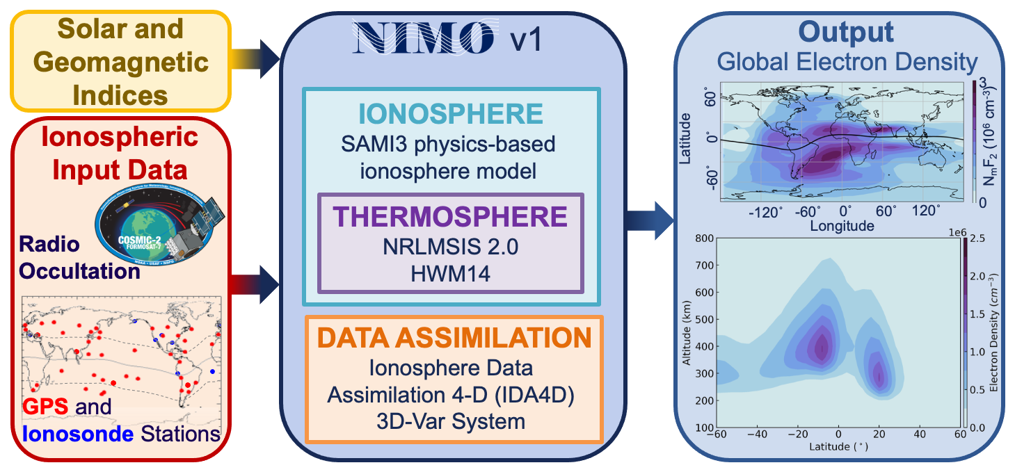
Figure 1 NIMO consists of a data assimilation system, IDA-4D, and a physics-based ionosphere model, SAMI3. NIMO ingests a number of different data sets that can be represented as an electron density. The output is a 3D representation of the ionospheric electron density over the entire globe.

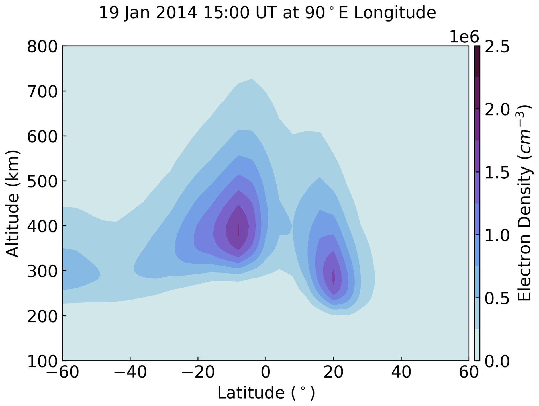
Figure 2 NIMO specification of electron density as a function of latitude and altitude at a longitude of 90° E at 15:00 UT for 19 January 2014.

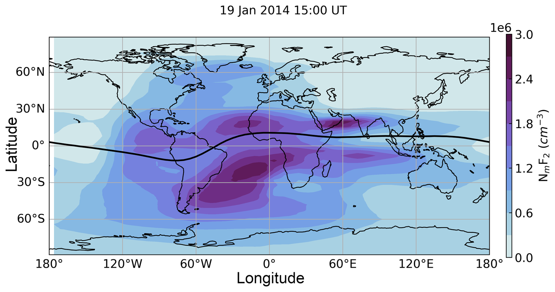
Figure 3 NIMO specification of global peak electron density in the F region at 15:00 UT for 19 January 2014.

The design of NIMO is similar to that of numerical weather forecast systems in that it consists of a forecast model and Data Assimilation (DA) system that runs in real time to generate both analysis states and weather forecasts at a regular cadence. The NIMO forecasts, as well as the background ionospheric state for the DA system, are generated by SAMI3 (SAMI3 is also a Model of the Ionosphere), which is a physics-based model of the ionosphere developed at the Naval Research Laboratory (NRL) (Huba et al., 2000, 2008, 2019). The DA is performed by the Ionospheric Data Assimilation Four-Dimensional (IDA-4D) system. IDA-4D uses a mathematical formulation that closely follows the meteorological 3D Variational Assimilation (3DVar) methodology and is described in detail in Bust et al. (2004, 2007).

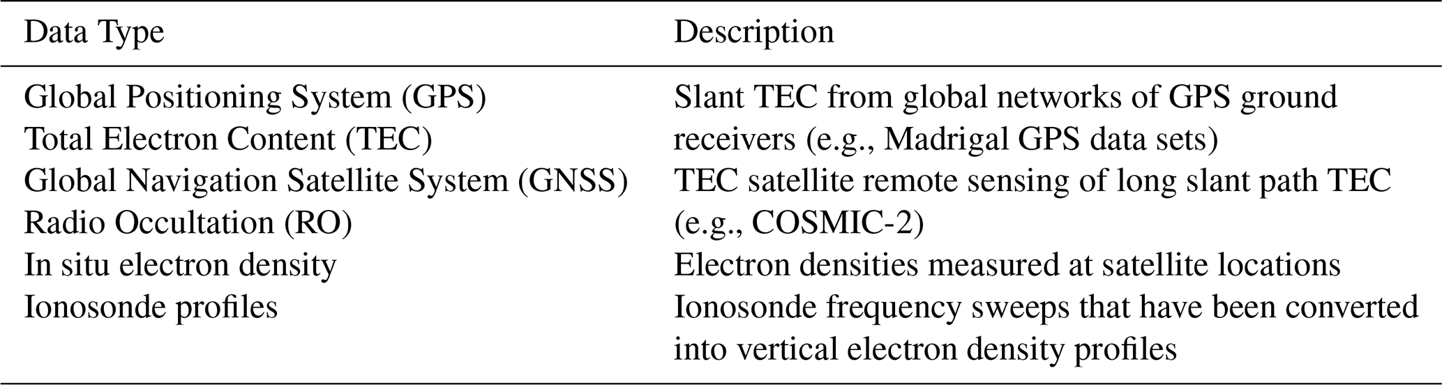
NIMO includes a data pre-processor that reads in the various data sets, performs checks to verify the data is usable, and generates a file with all the data that will be assimilated within a given time step. The code was designed to be easily extensible to new data sources as they become available. This was done by requiring only that the data be manipulated to provide some form of electron density and a grid specifying the data locations in geographic coordinates. The extensibility of the data pre-processor to new data sets has been tested with multiple data sources not included in this study, including Total Electron Content (TEC) derived from lightning measurements (Lay et al., 2022) and nighttime ultraviolet (UV) measurements of oxygen airglow from the Special Sensor Ultraviolet Limb Imager (SSULI) and Special Sensor Ultraviolet Spectrographic Imager (SSUSI) instruments aboard the Defense Meteorological Satellite Program (DMSP) satellites. Supported real-time data sets for NIMO v1.0 are listed in Table 1. As noted previously, more recent versions of NIMO (v1.2 and greater) have successfully added the capability to ingest UV radiance observations from SSULI and SSUSI.

Table 1 Data types that can be ingested into NIMO version 1.0.

Because IDA-4D is a 3DVar system, all the data collected within a single iteration is assimilated at the same time. Due to the highly variable nature of the ionosphere, we have set this iteration step to be 15 min. Thus, every 15 min NIMO collects the available operational data sets for the current time period, ingests them into the data pre-processor, and performs the assimilation with IDA-4D using the SAMI3 background state from the previous time step.

The data pre-processor uses a Gauss-Markov filter to update the background electron density state with the model errors based on an empirical model of the model covariance consisting of three independent Gaussian distributions in magnetic longitude, magnetic latitude, and geographic altitude (details found in Bust et al., 2004; Bust and Datta-Barua, 2014). The IDA-4D electron densities are then provided on a global geographic longitude, latitude and altitude grid (extending up to 10 000 km). These geographic locations are interpolated onto the SAMI3 magnetic grid using the Earth System Modeling Framework (ESMF) by Collins et al. (2005) and partitioned into the SAMI3 ion constituents using ratios determined in the previous time step.

SAMI3 then runs forward 15 min to generate the background state for the next iteration. NIMO may be run in hindcast or real time mode, depending on the needs of the user. NIMO also generates short-term forecasts; however, because IDA-4D is only updating the SAMI3 ion densities, and not thermospheric or electromagnetic drivers of the ionosphere, the NIMO forecasts revert to free-running SAMI3 within 30 min to several hours depending on the location, local time and geomagnetic conditions. For the purposes of this study, only the hindcast mode is used and forecasts are not evaluated.

3 Model Configuration

This section provides a summary of the model configuration and data sets used to perform the validation runs.

3.1 SAMI3 and IDA-4D Configuration

For global runs, such as presented here, SAMI3 is configured to run with a low-resolution grid that has 160 points along each magnetic field line, 160 field lines at each magnetic longitude, and 90 magnetic longitude slices. This grid yields a 4° resolution in longitude and 1° resolution in latitude and extends from 70 km to greater than 20 000 km in altitude. The auroral model and high-latitude convection model are not used in these runs, as further testing is required for their integration. The NIMO thermosphere is specified by the Horizontal Wind Model (HWM14; Drob et al., 2015) and the NRL Mass Spectrometer Incoherent Scatter (NRLMSIS-2.0, Emmert et al., 2021). Solar and geomagnetic inputs are provided by the 10.7 cm solar radio flux (F_10.7), three-hour a_P (a linear measure of the planetary geomagnetic disturbance level), and the 81 d, centered average of the F_10.7 (F_10.7a).

Within the NIMO validation runs, IDA-4D was configured with a global equal area grid with 300 km grid spacing in latitude and longitude, and altitudes ranging from 100 to 1500 km. The January 2021 global run was performed with two different IDA-4D grids. These grids differed in the range of their topside altitudes, in operations the IDA-4D grid extended up to 10 000 km. Although not used in the standard validation runs, the newer IDA-4D grid led to a small improvement in the ionospheric specification.

An early version of NIMO, called IDA-4D/SAMI3, ingested non-real time GPS data from ground stations available from the International Global Navigation Satellite System (GNSS) Service with a 5 min assimilation time step to study localized enhancements of electron density following geomagnetic storms (Chartier et al., 2021). In this study, IDA-4D/SAMI3 N_mF₂ was validated for two storm periods in November 2003 and August 2018 using in situ electron density data, autoscaled ionosonde N_mF₂ and reference GPS data. The assimilation model was found to reduce the Root Mean Squared Error (RMSE) of N_mF₂ in SAMI3 by up to 35 %–50 %. This early version of the model was functionally similar to NIMO v1.0. The primary difference between IDA-4D/SAMI3 and NIMO v1.0 is that the pre-processor portions of IDA-4D were moved into a separate routine and the code was reconfigured to run in real-time.

3.2 Ingested Data Sets

Data sets ingested for the validation runs include Global Positioning System (GPS) relative Total Electron Content (TEC) (Martire et al., 2024), Electron Density Profiles (EDPs) from the National Oceanic and Atmospheric Administration (NOAA) Mirrion 2 ionosondes (McNamara, 2005; National Centers for Environmental Information, 2025), and space-based radio occultation (RO) data. The ionosonde EDPs come from the .EDP files on the NOAA database. The RO data is obtained from the Constellation Observing System for Meteorology, Ionosphere, and Climate (COSMIC) and COSMIC-2 constellations, which is publicly available at the University of Colorado (UCAR COSMIC Program, 2019, 2022). NIMO processes the slant TEC from the podTEC files. NIMO is also capable of ingesting commercial RO data (such as data sets provided by Spire and GeoOptics).

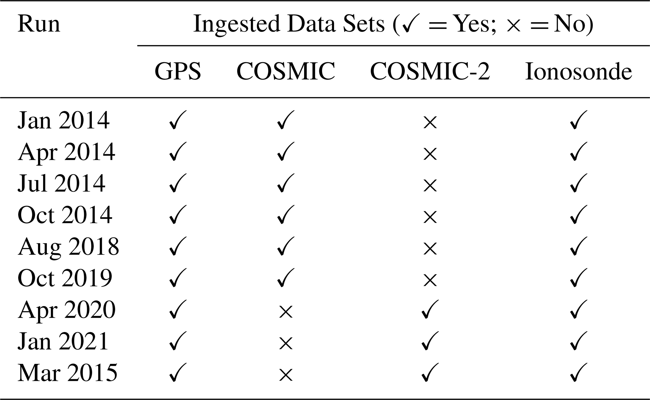
The data included in each of the different validation runs are shown in Table 2. The combination of ground- and space-based observations leads to reasonable global coverage, though there is less data to ingest at high latitudes and over the oceans.

Table 2 Data ingested for the validation runs tabulated in Table 3.

4 Model Validation

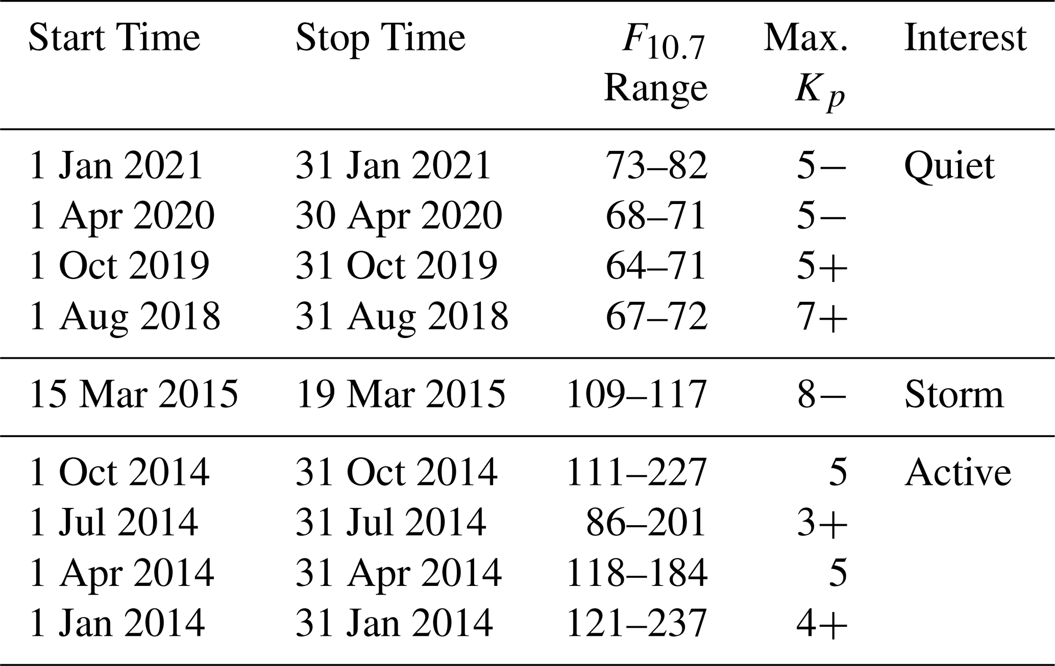
The purpose of this validation is to evaluate the accuracy of the electron density against observations in different spatio-temporal regions, ionospheric layers, and under different solar and geomagnetic conditions for the global NIMO runs. A variety of different validation periods, shown in Table 3, were chosen to ensure representative seasonal and solar cycle coverage under quiet geomagnetic conditions. An additional run that includes a significant geomagnetic storm is also considered to allow evaluation during disturbed geomagnetic times, bringing the total of runs up to nine.

Table 3 Validation periods.

The validation process involves establishing meaningful comparison metrics from different observational or empirical data sets and evaluating the new model's performance against the International Reference Ionosphere (IRI-2016), a climatological model primarily based on ionosonde measurements (Bilitza, 2018). The IRI-2016 was run using a compiled executable with the default flags as of Sep 2021, except for the h_mF₂ model, which was set to SHU-2015 Shubin (2015). The SHU-2015 model was set as the default for IRI-2016 in October 2021.

IRI-2016 was chosen to compare against because it was the most up-to-date version at the time this validation was performed. Since 2014, IRI has been recognized as the official standard for the Earth's ionosphere by the International Standardization Organization (ISO) (ISO 16457:2014, 2014; ISO 16457:2022, 2022). It is similarly endorsed by the International Union of Radio Science, the Committee on Space Research, and the European Cooperation for Space Standardization (Bilitza et al., 2022). Future versions of NIMO and other ionospheric models (empirical, first-principles, or assimilative), may compare their performance against these results.

IRI-2016 was run at a one hour temporal cadence with a 5° N × 4° E× 10 km latitude × longitude × altitude grid. The altitude range was chosen to allow the Joint Altimetry Satellite Oceanography Network (JASON) TEC to be compared against modeled TEC calculated up to the altitude of 1300 km, similar to the nominal orbital altitude. Some of the validation methods interpolate between these times, while others simply calculate statistics at a lower cadence. The interpolation method showed little difference in results between a one hour resolution and a 15 min resolution, as IRI-2016 varies smoothly. The matching method was found to work well as long as enough paired data points were available to calculate the desired statistics.

Seven different observational data sets and one empirical model were used to calculate validation metrics for this study. Each data set has its own intricacies, which are discussed in Sect. 4.1. Finally, the different metrics used in this validation study are presented in Sect. 4.2.

4.1 Data Sources

This section provides an overview of the ground- and space-based observational data sets used to validate the electron density provided by NIMO.

4.1.1 Ionosondes

Ionosondes measure the time delay of vertically propagated Medium Frequency (MF) and HF radio waves (the combined MF-HF range spans from 0.3 to 30 MHz), which reflect off of the bottomside of the ionosphere. The transmitter sweeps through a subset of the MF and HF range to obtain information about the electron density at multiple altitudes. To analyze ionosonde data, the frequency-altitude output must be scaled and inverted from delay as a function of frequency to electron density as a function of altitude. This can be done using an auto-scaler program or performed manually by an experienced analyst. The data for these validation studies was collected from the Lowell GIRO Data Center (LGDC), which collects data from ionosondes around the world (Reinisch and Galkin, 2011). The majority of the validation data in this study has been scaled using versions 4, 4.5, and 5 of an autoscaler called Automatic Real-Time Ionogram Scaler with True height (ARTIST), although some of the outputs from LGDC indicate that the scaling method used is unknown (Galkin and Reinisch, 2008). These were likely scaled by other autoscalers used by different institutions. The ARTIST outputs do not include errors in the measurements but they do include a confidence score that can be used to determine if the profile is usable.

Using hand-scaled ionograms is generally considered preferable to using autoscaled ionograms, since the results have been verified by a knowledgeable data processor. However, it can be very time consuming and the results may not be available for a real-time operational validation. Themens et al. (2022) discusses the challenges and best practices for using ARTIST autoscaled parameters. They describe how to use the autoscale scores and conclude that it varies depending on parameter and is not as simple as using a cutoff value. Based off this analysis, we use a cutoff of 70 for both f_oF₂ and h_mF₂ to use the same times for both analyses. In Galkin et al. (2008) they discuss the f_oF₂ error for three sites by comparing the f_oF₂ to hand scaled ionosondes. They found that 95 % of automatically determined f_oF₂ from ARTIST 5 fell within −0.3 to 0.4 MHz of the hand scaled profiles. The hand scaled profiles also have errors associated with them that are harder to quantify. Only auto-scaled ionosondes were used in this study to replicate what would done in a real-time verification. Since the autoscale confidence score does not catch all issues in scaling, it is likely that poorly scaled ionosonde data were included in the data validation, despite efforts to ensure a clean data set. The ingested data uses a different error analysis and may also include poorly scaled data.

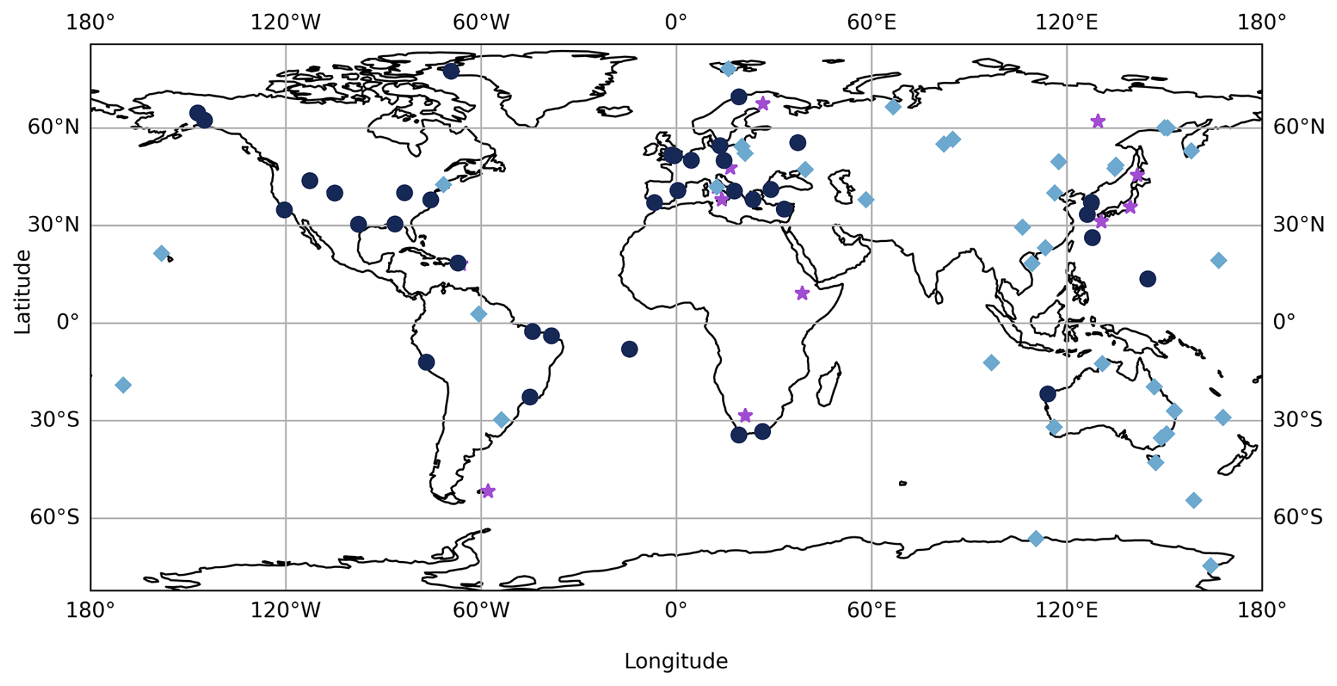
Figure 4 Map of ionosonde locations used for data assimilation and validation. The purple stars are sites that are only used for data assimilation. The light blue diamonds are sites that are used for validation only. The navy circles are sites that are used for ingestion and validation.

Ionosondes are relatively inexpensive instruments to install and operate, making them a popular source for ionospheric measurements across the globe. Figure 4 shows the locations of the sites used in this study for both assimilation and validation. Different time periods are used in this study, so different ionosondes are used for assimilation and validation for each run. For each model run, not every ingested site and not every validation site from the map is used. Sites that are used for assimilation and ingestion were ingested for at least one of the runs and also used to validate at least one run but for any given time period they may not have been used for both ingestion and validation. Additionally, since the assimilated data are processed differently from the validation data, the ingested data is not identical to the validation data at these sites that are used for both. When specific ionosonde sites are used for validation, they are identified by station name and location. Another complication for this validation effort is that some of these ionosondes are also used in NIMO's data assimilation. The NOAA Mirrion 2 ionosonde database includes some of these ionosondes, but not all of them. This database also includes ionosondes that are not included in the validation. Although the ingestion process does remove some of the provided data to prevent the dominance of one data set on the assimilation, this information is not available post-processing. Due to this complication, instances where ionosonde data is or is not assimilated are addressed on a case-by-case basis and the regional statistics do not make a distinction between these two possible states. Additionally, the distribution of ionosonde locations means global statistics will be biased towards mid-latitude results.

4.1.2 Incoherent Scatter Radars

An Incoherent Scatter Radar (ISR) probes the ionosphere through very weak stochastic collective Thomson backscatter from thermal electrons in the ionosphere, electrostatically modified by the presence of ions (Dougherty and Farley, 1960). The very weak nature of the scatter allows full altitude profiles of plasma parameters into the topside ionosphere. The ISR systems need to be large and powerful (Farley, 2009), since the electron radar scattering cross-section is roughly 10⁻²⁸ m² and the plasma in the ionosphere is at least 90–100 km away. There are only six ISR systems in the American sector, located in Alaska, Nunavut (Canada), Massachusetts, Puerto Rico, and Peru. This study uses the available ISR data, which comes from the Millstone Hill (MH), Arecibo Observatory (AO), and Jicamarca Radio Observatory (JRO) ISRs.

The MH ISR is operated as part of the Millstone Hill Geospace Facility at the Haystack Observatory, a sub-auroral/mid-latitude location (42.62° N, −71.95° W). This ISR transmits 2.5 MW maximum peak power at Ultra-High Frequencies (UHFs, ranging from 300 MHz to 1 GHz), and has a wide field of view with a 46 m fully steerable antenna and a 68 m zenith/vertical antenna. The data presented in this document were acquired with the fixed zenith antenna using an interleaved combination of uncoded and alternating code (Lehtinen and Häggström, 1987) waveforms, and yields a changing altitude resolution from 4.5 km at the E region to less than 60 km at an altitude of 400 km. MH data uses a radar calibration constant to yield absolute electron density values; two different methods of obtaining electron density profiles were used for the experiments in this study. Before 2015, MH “ion line” observations, yielding full altitude plasma parameters including electron density, were calibrated against F₂ region peak electron density values from the co-located UM Lowell digisonde (station code MHJ45) at the observatory. After 2015, MH “ion line” observations were self-calibrated to simultaneous extremely weak but precise F₂ peak altitude Langmuir mode/“plasma line” observations, which by their nature produce absolute electron density referenced to fundamental physical constants.

The AO is located in Puerto Rico at (18.3° N, 66.7° W), and is considered a low-latitude site. It had the largest single dish ISR until 2019, when it ceased operations. The ISR instrument consisted of two 430 MHz radar antennas that could be used together or independently, in addition to other antennas that transmitted different frequencies used for radio astronomy, planetary, and HF studies. The Arecibo ISR had the highest sensitivity among all ISRs, with range resolution of 150 m, time resolution of the order of ms, and frequency resolution of 0.7 kHz. The data in this study uses the calibrated ion line to validate the NIMO simulations.

The JRO is located in Peru at (11.9° S, 76.9° W), under the magnetic equator, with a magnetic dip angle around 1°. The JRO ISR is an array of 18 432 crossed-dipole 50 MHz antennas, covering an area of 85 000 m², that transmits up to 4.5 MW of power. The JRO ISR dual-polarization makes it possible to measure the Faraday rotation of the incoherent backscatter waves, which allows an absolute estimate of electron density independent of any other instrumentation (Farley, 1969). The range resolution of the data is set by the radar transmitted codes (Hysell, 2018). JRO uses alternate uncoded pulses that minimize the clutter at F region heights and provide a height resolution of 15 km.

4.1.3 GNSS TEC

TEC is measured by satellite-based transmitters paired with either ground- or space-based receivers that measure the time delay between signals at two different frequencies. The TEC provides a column integrated density measurement rather than vertically resolved electron density profiles, but the high accuracy and vast coverage of this data set make it, arguably, the most complete ionospheric specification data set currently available.

The TEC measured by distributed ground- and space-based receivers and transmitters onboard the GNSS satellite constellation provide line-of-site, or slant TEC (STEC), measurements of the density along the path between the transmitter and receiver. This path typically covers a range of latitude and longitudes, and so is frequently converted to vertical TEC (which projects the STEC vertically using assumptions about the ionospheric structure). The Massachusetts Institute of Technology (MIT) Haystack Madrigal database provides two TEC products as part of Millstone Hill Geospace Facility TEC analysis operations: the STEC and unbinned vertical TEC as well as vertical TEC binned at a resolution of 5 min, 1° latitude and 1° longitude (Rideout and Coster, 2006; Coster, 2026). The sources of uncertainties and biases in the TEC processing are reported in Rideout and Coster (2006) and Vierinen et al. (2016), and the gridded vertical TEC files report data errors for each gridded value. These errors typically range between 0.1 and 1.0 TEC Unit (TECU) (where 1 TECU = 10¹⁶ electrons m⁻²) over the validation region. Figure 5 shows the typical coverage of the vertical TEC data with the area used for validation marked by a green box.

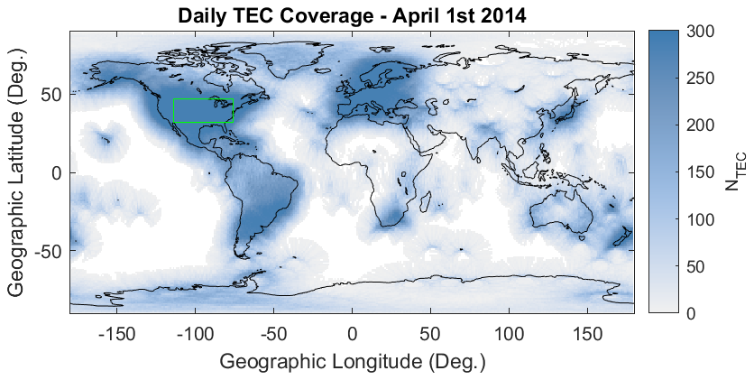
Figure 5 Madrigal binned TEC coverage for 1 April 2014 where N_TEC is the number of observations at each location over the selected day. The green square marks the validation region.

As was the case with the ionosonde data, TEC was also ingested into the NIMO data assimilation. However, in this instance the assimilated TEC was obtained from a different source and does not retain any information about the receiver bias calibration, as the relative TEC (not the total slant or vertical TEC) is assimilated. Thus, the validation data set will be distinct from the assimilated data set, even if the same satellite-receiver pairs are used, especially when considering statistics such as the bias.

4.1.4 JASON TEC

The JASON satellites are part of a mission to supply scientific and commercial data about sea level rise, ocean temperatures and circulation, and climate change. The JASON-3 satellite launched in 2016 and is still operational, and so covers many of the validation periods shown in Table 3. The validation periods in 2014 are covered by JASON-2, which was operational between 20 June 2008 and 9 October 2019. These satellites include dual-frequency altimeters, operating at 13.575 GHz (K_u-band) and 5.3 GHz (C-band), to measure the height of the ocean surface to high accuracy. The JASON satellites fly in an orbit with a 66° inclination and a 10 d repeating reference orbit, advancing approximately 2° d⁻¹.

Corrections must be applied to these measurements due to the dispersive nature of the atmosphere that results in path delay of the radar signal. The ionospheric correction, or delay, is directly proportional to the electron content along the ray path and inversely proportional to the frequency (f) squared of the signal. The difference in delay between the altimeters’ dual-frequency measurements can be used to calculate the TEC in the nadir (vertical) direction from the spacecraft at 1340 km altitude to the surface over the oceans (Imel, 1994). TEC is calculated using the following formula:

$$\begin{array}{}\text{(1)}& \mathrm{TEC}=-\mathrm{dR}\times {\displaystyle \frac{f^{\mathrm{2}}}{\mathrm{40.3}}}\end{array}$$

In Equation 1, TEC is the vertical TEC in the ionosphere measured in TECU, dR is the K_u-band ionospheric range correction in meters provided in the JASON-2 and JASON-3 Geophysical Data Records (GDRs) that are available at, for example, https://www.ncei.noaa.gov/data/oceans/jason3/gdr/gdr/ (last access: 7 October 2025) (NOAA/NESDIS Office of Satellite and Product Operations, 2008; Lillibridge and US DOC/NOAA/NESDIS > Office of Satellite Data Processing and Distribution, 2019). The sampling rate of the JASON-2 and JASON-3 instruments is 1 Hz. However, as recommended by Imel (1994) and the JASON-3 Handbook (Dumont et al., 2017), the ionospheric range correction should be smoothed over 100 km or more to reduce instrument noise. To calculate the JASON-2 and JASON-3 TEC used in this study, we have averaged the measurements over 18 s, which yields approximately ∼ 1° bins. The $\frac{\mathit{\sigma }}{\sqrt{N}}$ precision is ∼ 1 TECU. Because both JASON-2 and JASON-3 satellites are used in this validation study, we have been careful to take the bias between the instruments into account. During the tandem period (February–October 2016), JASON-3 was inserted into the same orbit as JASON-2 and trailing by one minute. An evaluation of the TEC measurements during this time period shows that the JASON-2 instrument has a +2.6 TECU bias with respect to the JASON-3 instrument. For this study, we have subtracted 2.6 TECU from the JASON-2 measurements to account for this bias.

While JASON-3 does not provide a dense set of measurements, it does provide a direct TEC measurement over bodies of water. Altimeter data, such as this, has been used extensively to validate TEC models and other measurement techniques (e.g., Burrell et al., 2008; Li et al., 2018).

4.1.5 CINDI

The Coupled Ion-Neutral Dynamics Investigation (CINDI) mission operated onboard the Communication/Navigation Outage Forecasting System (C/NOFS) satellite (de la Beaujardière and C/NOFS Science Definition Team, 2004) between 2 August 2008 and 26 November 2015. The C/NOFS satellite was launched into a low earth orbit with an inclination of 13° and an orbital period of about 97 min. Initially, the satellite orbit had a perigee of 400 km and an apogee near 860 km. The mission was placed in safety mode (not providing any data) between 5 June 2013 and 22 October 2013, before becoming operational again (at this point the C/NOFS satellite had a perigee of 388 km and apogee of 690 km). This orbit allowed the orbital plane to precess 24 h in local time over a period of 3 months.

Two instruments from the CINDI mission are used in the data validation efforts: the Retarding Potential Analyzer (RPA) and the Ion Drift Meter (IDM) (Heelis and Hanson, 1998). Together known as the Ion Velocity Meter (IVM), these instruments provided the 3D ion velocity, converted into magnetic coordinates using the International Geomagnetic Reference Field (IGRF) (Maus et al., 2005), as well as the ion density, temperature, and composition. The pysat data framework (Stoneback et al., 2018, 2021) includes cleaning routines for these instruments, ensuring a high quality of data when performing validations (Stoneback et al., 2011; Burrell, 2012). The orbital characteristics of the C/NOFS satellite allow CINDI observations to validate model runs in the topside, equatorial ionosphere. The data files were retrieved from the NASA Space Physics Data Facility (, ).

4.1.6 DMSP SSIES

The DMSP Special Sensor for Ions, Electrons, and Scintillation (SSIES), an earlier incarnation of the CINDI IVM, was flown onboard four of the DMSP satellites (F15, F16, F17, and F18) as a part of their mission is to monitor the meteorological, oceanographic, and geospace environment (Hall, 2001). The first DMSP satellite was launched in 1962, and there are currently several satellites operational and in their desired orbits. These orbits are sun-synchronous, polar orbits with altitudes near 830 km. Each satellite crosses the equatorial plane at a different Solar Local Time (SLT), allowing DMSP to validate the topside ionospheric density at a range of latitudes and local times. DMSP SSIES data (Level 1 processing) was processed by Boston College and retrieved from the CEDAR Madrigal database (Groves, 2026).

4.1.7 ICON IVM

The Ionospheric CONnection Explorer (ICON) IVM suite measured the in situ ionospheric drift (Heelis et al., 2017) using RPAs and IDMs at the front (A) and rear (B) of the spacecraft. For the periods used in this validation study, only IVM-A returned observations. The IVM measures the ion density, temperature, 3D drift, and composition. The ion density, which is the density for all species, may be directly compared to the model's electron density as there are only significant populations of singly-ionized species in the topside ionosphere. The data files were retrieved from the NASA SPDF (, ).

4.2 Validation Metrics

This section describes the metrics that are used to evaluate the model. Here and elsewhere, the subscript obs is used to indicate observational data, while the subscript mod indicates modeled data. When two different models are being compared, subscripts will use the model names.

A variety of metrics were employed in this validation. Each metric provides slightly different insight into the model performance and has different weaknesses, and so it was determined that a single metric is not desirable for a comprehensive validation effort. The different observation data sets do not all report an identical set of metrics, due largely to the ease of performance interpretation. For example, the topside plasma density validation using CINDI, ICON, and DMSP uses the median absolute error to reduce the impact of outliers, while the ionosondes used the mean absolute error because the larger quantity of data made outliers less impactful. Despite these differences, all data sets do report the bias (Sect. 4.2.2), allowing a consistent evaluation of the model performance across all observations for this metric.

4.2.1 Difference Histograms

A standard way of visualizing the agreement between two data sets is to plot a histogram of the differences between the two data sets. If there is no systematic offset between the two data sets and any disagreement is randomly distributed, the histogram will have a classic Gaussian bell shape centered about zero. The offset of the peak, pronouncement of the tails, and symmetry of the distribution at the half-maximum point can all be easily assessed using a difference histogram.

4.2.2 Bias or Mean Error

The Bias (B) or the Mean Error (ME) is a scale-dependent bias, measured by differencing the means of two data sets, as shown in Eq. (2). As previously stated, the subscript mod refers to model data and the subscript obs refers to observational data. X acts as a placeholder for the different observations used in the validation efforts, and 〈X〉 denotes the mean of the enclosed data set. B and ME are the same statistic.

$$\begin{array}{}\text{(2)}& B=\langle X_{\mathrm{mod}}\rangle -\langle X_{\mathrm{obs}}\rangle \end{array}$$

4.2.3 Root Mean Squared Error

The Root Mean Squared Error (RMSE) provides a measure of the magnitude of the difference between two data sets. It is defined as:

$$\begin{array}{}\text{(3)}& \mathrm{RMSE}=\sqrt{\langle {\left(X_{\mathrm{mod}}-X_{\mathrm{obs}}\right)}^{\mathrm{2}}\rangle }.\end{array}$$

4.2.4 Mean Absolute Error

The Mean Absolute Error (MAE) is another way to measure the magnitude of the difference between two data sets. Described in Eq. (4), it is simply the mean of the absolute value of the difference between the modeled and observed data sets.

$$\begin{array}{}\text{(4)}& \mathrm{MAE}=\langle |X_{\mathrm{mod}}-X_{\mathrm{obs}}|\rangle \end{array}$$

4.2.5 Median Absolute Error

The Median Absolute Error (Med. AE) is a more robust measure of the magnitude of the difference between two data sets. It is calculated in the same way the MAE is, but instead of taking the mean of the absolute value of the differences between the modeled and observational data sets, the median is calculated. This makes the result less susceptible to outliers, but it does not measure the distribution of differences between the data pairs.

4.2.6 Mean Absolute Percentage Error

The Mean Absolute Percentage Error (MAPE) is a way to measure the magnitude of the difference between two data sets. Described in Eq. (5), it is simply the mean of the absolute value of the difference between the modeled and observed data sets, expressed as a percentage.

$$\begin{array}{}\text{(5)}& \mathrm{MAPE}=〈{\displaystyle \frac{|X_{\mathrm{mod}}-X_{\mathrm{obs}}|}{X_{\mathrm{obs}}}}〉\times \mathrm{100}\mathit{\%}\end{array}$$

4.2.7 Pearson Correlation Coefficient

Correlation coefficients are a way to show how strongly two sets of data are related. The Pearson correlation coefficient (r₁) measures the strength of the linear correlation between two sets of data by determining the ratio between the covariance of two variables and the product of their standard deviation. Positive values indicate a strong association among the two sets, negative values indicate an anti-correlation, and values equal to zero indicate no relationship at all. The correlation of a set of data with itself gives an r₁ of unity. The Pearson correlation coefficient equation between the modeled and observed data sets is calculated using:

$$\begin{array}{}\text{(6)}& r_{\mathrm{1}}={\displaystyle \frac{{\sum }_i^N(X_{{\mathrm{mod}}_i}-\langle X_{\mathrm{mod}}\rangle )(X_{{\mathrm{obs}}_i}-\langle X_{\mathrm{obs}}\rangle )}{\sqrt{{\sum }_i^N(X_{{\mathrm{mod}}_i}-\langle X_{\mathrm{mod}}\rangle {)}^{\mathrm{2}}{\sum }_i^N(X_{{\mathrm{obs}}_i}-\langle X_{\mathrm{obs}}\rangle {)}^{\mathrm{2}}}}}.\end{array}$$

In the above equation, N is the number of samples and i is the index of an individual model-observation pairing.

Correlation and anti-correlation can be differentiated together from the absence of any correlation by using the square of the Pearson correlation coefficient (R²). R² is simply the square of r₁, and is useful for separating data sets that have a relationship from those that have no relationship at all.

4.2.8 Meta Analysis

Meta analysis is commonly performed to obtain a clear picture of a large number of statistics. This study uses meta analysis to clarify the comparative model performance of one particular statistic. More specifically, when evaluating the performance of one of the statistics presented above (S), the percentage of validation runs where NIMO outperforms IRI-2016 (P_S) can be determined using:

$$\begin{array}{}\text{(7)}& P_S={\displaystyle \frac{{\sum }_i^{N}c\left(i,\mathrm{NIMO},\text{IRI-2016}\right)}{N}}\times \mathrm{100}\mathit{\%},\end{array}$$

where:

$$\begin{array}{}\text{(8)}& \begin{array}{rl}c& \left(i,\mathrm{NIMO},\text{IRI-2016}\right)\\ & =\left\{\begin{array}{ll}\mathrm{1},& \mathrm{if}{S}_{i_{\mathrm{NIMO}}}\mathrm{is}\mathrm{better}\mathrm{than}{S}_{i_{\text{IRI-2016}}}\\ \mathrm{0},& \text{otherwise}.\end{array}\right.\end{array}\end{array}$$

In the equations above N is the number of validation runs. The qualifier “better than” is used instead of a numerical description because the numerical condition that indicates a “better” value changes. For example, the RMSE is better when the value is lower, but the B is better when its absolute value is closer to zero.

4.3 Validation Results

4.3.1 Ionosondes

While ionosondes provide a wealth of data that can be used to validate several different aspects of the bottomside ionosphere, this study uses only the f_oF₂ and the h_mF₂. This choice was made to ensure that the most reliable aspects of the auto-scaled ionosonde data were used in the validation process. Focusing on the critical frequency and height of the F₂ peak has the additional advantage of validating the location and strength of a major ionospheric feature.

Figure 6 shows the observed and modeled f_oF₂ for a day at two of the ionosonde sites; the top panel shows data that was included in the data assimilation (Boulder, USA) and the bottom shows data that was not assimilated (Beijing, China). Ionosonde measurements are shown as red dots, the NIMO output is marked by a blue line and triangles and the orange line and squares shows the IRI-2016 output. NIMO shows significantly more variation than IRI-2016, as it is not a climatological model. Additionally, the top panel shows a solar quiet period, while the bottom panel shows a solar active period. This illustrates how NIMO is typically more successful than IRI-2016 at capturing the critical frequency (and therefore density) at the F₂ peak, whether or not data was assimilated at this location.

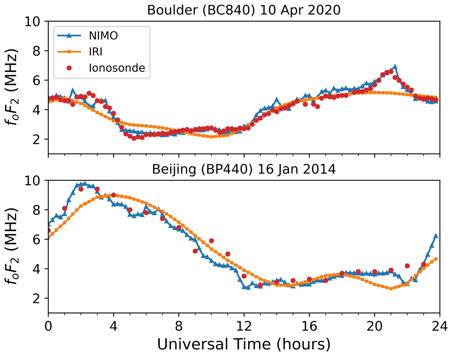
Figure 6 f_oF₂ for ionosonde station locations at Boulder, USA (top) and Beijing, China (bottom). The ionosonde observations are shown by red dots, while the NIMO results are plotted in blue lines and triangles and the IRI-2016 results are plotted in orange lines and squares.

However, it is more challenging to capture the correct h_mF₂. Figure 7 shows the same time periods and stations as Fig. 6, but for the h_mF₂. This demonstrates that the IDA-4D data assimilation process is also blindly successful, meaning that the model will attempt to drive the ionospheric state towards incorrect assimilated values and create unrealistic modeled output. At 01:30 UT the model fits a very high and unrealistic h_mF₂. The error in the EDP did match the true value of the error that was by determined by looking at the ionogram. All ionosonde values, even those with low confidence scores, are plotted here to show how the IDA-4D assimilation uses the data.

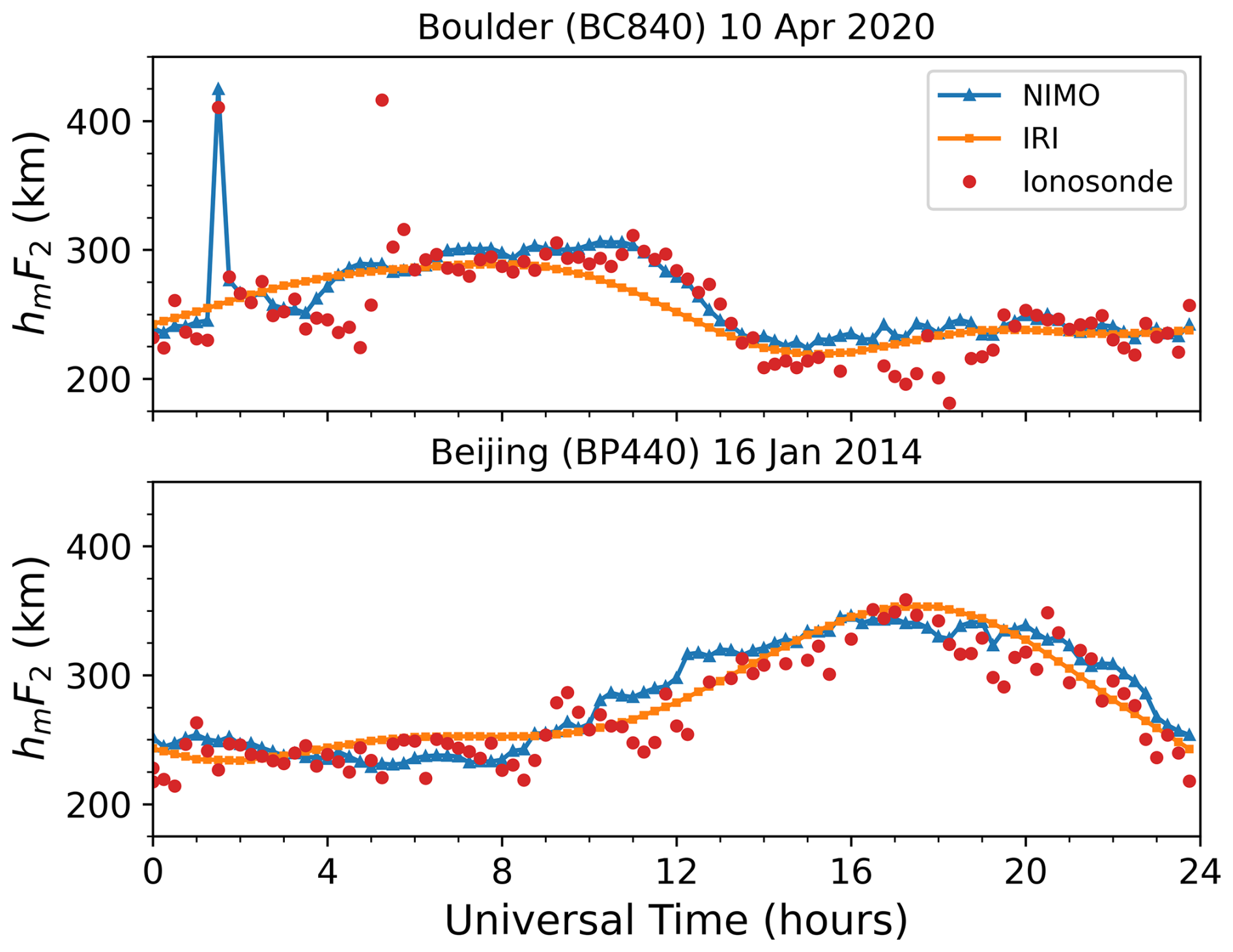
Figure 7 h_mF₂ for ionosonde station locations at Boulder, USA (top) and Beijing, China (bottom). The ionosonde observations are shown by red dots, while the NIMO results are plotted in blue lines and triangles and the IRI-2016 results are plotted in orange lines and squares.

The B, RMSE, and MAE (see Sect. 4.2.2, 4.2.3, and 4.2.4) are used to compare ionosonde observations with NIMO and IRI-2016 outputs. The global results from all available ionosondes are shown in Tables A1 and A2 and plotted in Figs. 8 and 9 for the desired validation periods. These statistics are calculated for all local times, daytime hours (06:00–18:00 SLT), and nighttime hours (18:00–06:00 SLT). Although these local times do contain some overlap of sunlit and non-sunlit locations (as solar zenith angle is not accounted for), they are each dominated by either day- or night-time processes. A subset of these runs was used to evaluate the f_oF₂ using only ionosondes not used in the data assimilation process (see Table 4).

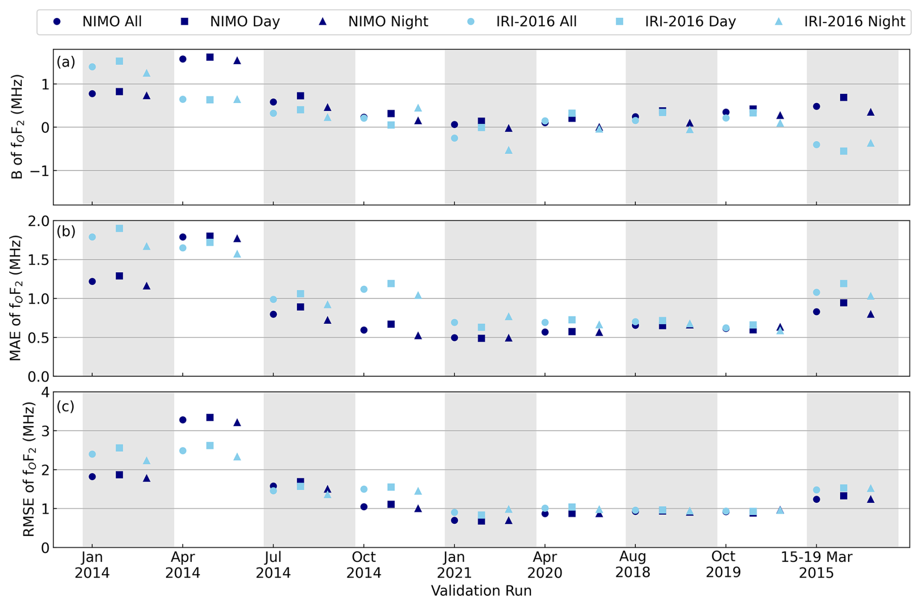
Figure 8 Global f_oF₂ B (a), MAE (b), and RMSE (c) in different local time bins for all ionosonde locations.

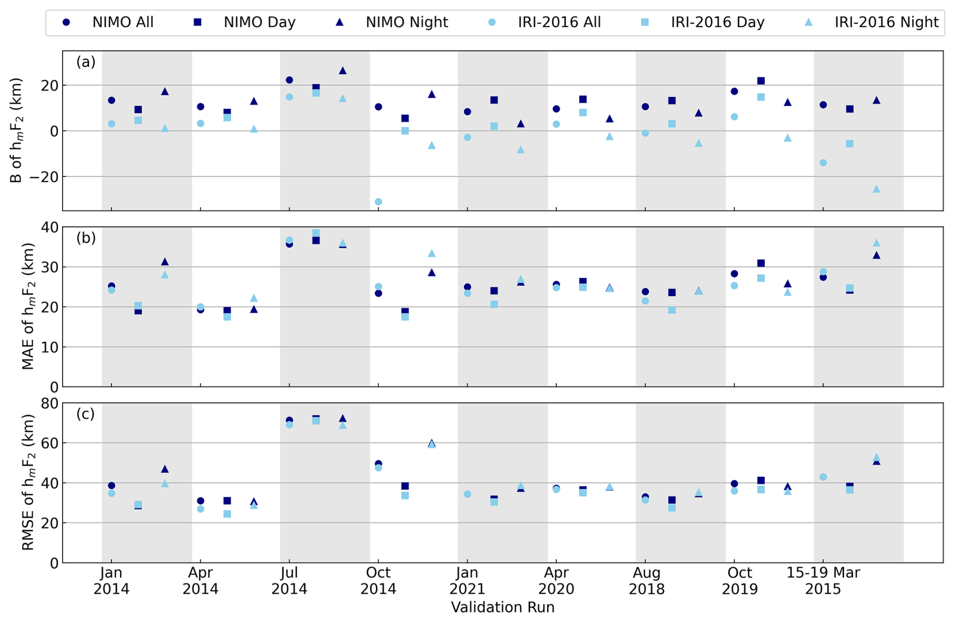
Figure 9 Global h_mF₂ B (a), MAE (b), and RMSE (c) in different local time bins for all ionosonde locations.

Table 4 Global, solar active f_oF₂ for all local times from only non-ingested ionosonde locations.

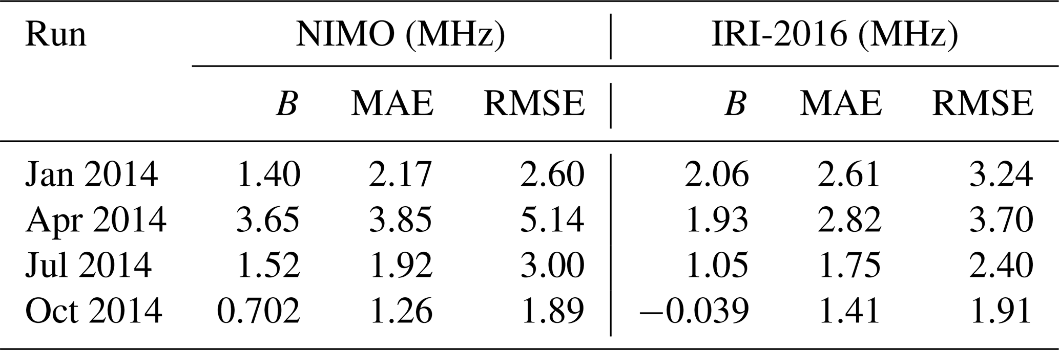
The B shows that both NIMO and IRI-2016 overestimate f_oF₂, while NIMO is more likely to overestimate the h_mF₂. In general, IRI-2016 tends to have a lower B than NIMO. Recall that a low bias may indicate a good performance or that a model is equally likely to overestimate as it is to underestimate for the chosen evaluation period. The interpretation that NIMO tends to overestimate the f_oF₂ and h_mF₂, while IRI-2016 overestimates peaks and underestimates minima for these values is supported by the examples shown in Figs. 6 and 7.

Examining the other f_oF₂ statistics further supports this interpretation. Calculating P_MAE for all validation runs and local time periods shows that NIMO performs better than IRI-2016 in 85.2 % of the cases. Similarly, P_RMSE=74.1 %. When considering the potential impact of removing the comparison with ionosondes used in the data assimilation, Table 4 shows that both NIMO and IRI-2016 have higher biases and errors for these four runs. However, the only time there is a change in relative performance between the two models is the July 2014 MAE, which is now lower for IRI-2016.

A challenge when using ionosondes for validation is that the errors from the ionosondes are not well defined, as previously discussed in Sect. 4.1.1. This impacts both the NIMO output, due to the ingested ionosondes, and the f_oF₂ and h_mF₂ validation with the ionosondes. Since this NIMO validation uses many ionosonde sites over long periods of time, it is likely that poorly-behaved ionosondes are included in the analysis. This will increase the error in an unquantifiable manner, but the robustness of the f_oF₂ and h_mF₂ parameters allows one to consider the ionosonde f_oF₂ as significantly more reliable than the ionosonde h_mF₂.

As expected due to the challenges with obtaining the h_mF₂, the validation against h_mF₂ is less consistent. IRI-2016 typically models the h_mF₂ better than NIMO, with P_MAE=44.5 % and P_RMSE=25.9 %. However, the difference between the MAE and RMSE values are usually less than 1 km, which is not significant.

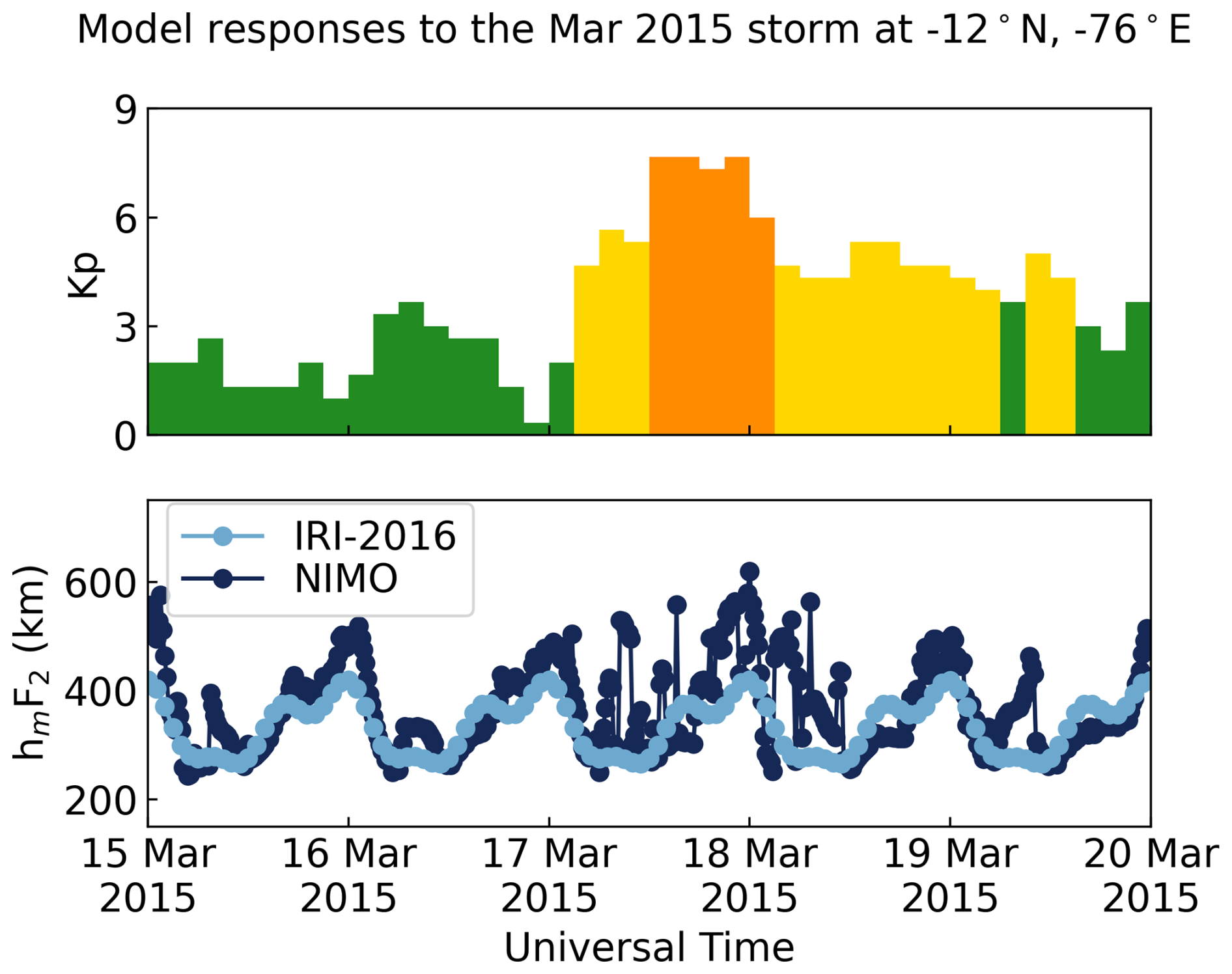
The run where NIMO most consistently performs better than IRI-2016 is the Mar 2015 storm period. During the geomagnetic storm, NIMO more correctly estimates the increases in f_oF₂ and h_mF₂ during the daytime and the nighttime. The nighttime differences between NIMO and IRI-2016 are more significant, though, with an improvement in the RMSE of 0.28 MHz for the f_oF₂ and 2 km for the h_mF₂. This is unsurprising, as NIMO better equipped to handle the combination of drivers needed to correctly specify an individual geomagnetic storm than a climatological model such as IRI-2016. Fig. 10 shows an example for NIMO (dark blue) and IRI-2016 (light blue) at a location near the Jicamarca Radio Observatory that demonstrates NIMO's ability to capture the expected uplifting of the F₂ layer caused by the geomagnetic storm.

Figure 10 K_p (top panel) and h_mF₂ (bottom panel) for the Mar 2015 storm period.

4.3.2 Incoherent Scatter Radars

The observations from ISRs located at AO, JRO, and MH were available for five of the desired validation periods: two active solar times, two quiet solar times, and the geomagnetic storm period. Following the lead of the ionosondes, the ISR data used for validation is currently limited to the h_mF₂ and N_mF₂. The h_mF₂ and N_mF₂ values for the ISR data are obtained by finding the maximum density and the corresponding altitude for each electron density profile at a given time.

Because NIMO captures both sub-hourly variations in the ionosphere and long-term climatological trends, it is useful to evaluate both the standard NIMO output and the trend of the NIMO output (which removes the short-term variations). The NIMO trend was calculated for the model's h_mF₂ and N_mF₂ by taking a boxcar average of the standard NIMO outputs using a full window width of 2 h. The trend results were provided at a 15 min resolution, matching the NIMO output cadence. A similar analysis was performed for the ionosonde validations, but the trend statistics were extremely close to the standard model statistics, and so are not included here in the interest of brevity.

The bias and the r₁ coefficient are calculated to determine both the degree and presence of a correlation between the models and the ISR observations. For the NIMO validation runs, the model trends for h_mF₂ and N_mF₂ are also examined to see whether NIMO captures the main features of the h_mF₂ and N_mF₂ in a manner comparable to IRI-2016. An example of the ISR data and model outputs is shown in Fig. 11, which shows the observations (purple), NIMO results (blue), NIMO trends (green), and IRI-2016 results (yellow).

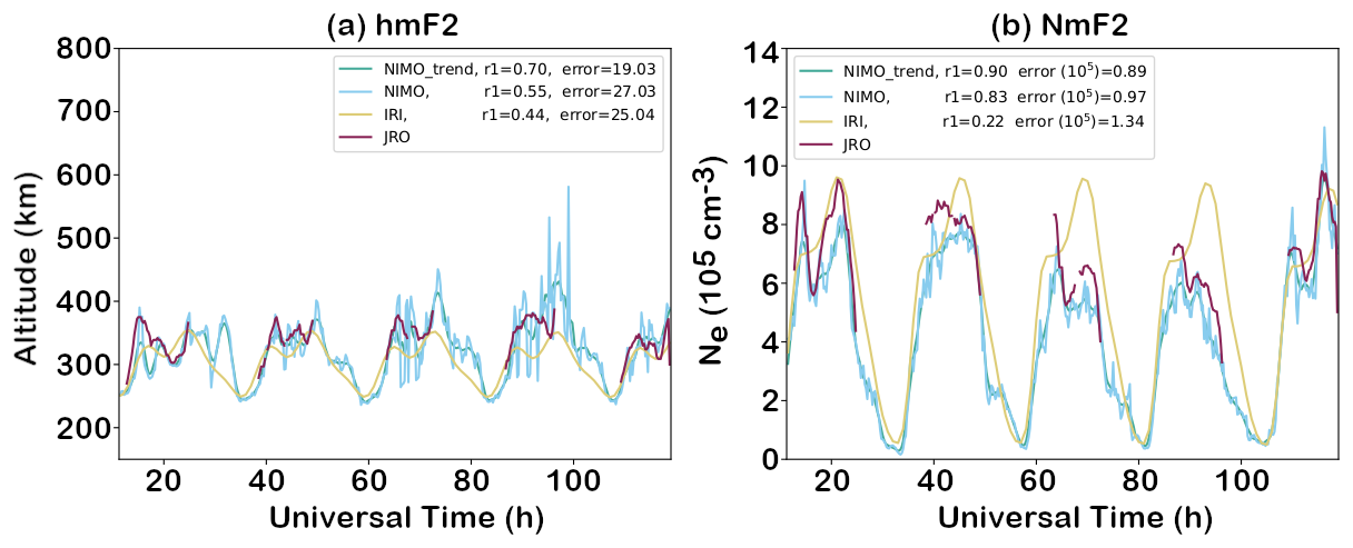
Figure 11 h_mF₂ (a) and N_mF₂ (b) for the JRO ISR starting at 6 January 2021 11:20 UT. The ISR observations are shown by purple lines, the NIMO results are plotted in blue, the NIMO trend is plotted in green, and the IRI-2016 results are plotted in yellow. Note how the purple JRO h_mF₂ generally lies in the middle of the NIMO h_mF₂ and shows similar local time variations to the NIMO N_mF₂, while the IRI-2016 values consistently have local time variations not consistent with the observations.

The results of the ISR h_mF₂ and N_mF₂ validation are shown in Figs. 12 and 13 (and presented in Tables A3 and A4), respectively. The results show that at all locations NIMO performs equally well or better than IRI-2016, when considering the standard model output and the NIMO trend. The NIMO trend usually performs slightly better than the standard NIMO output (except during the storm run), though the differences in the metrics are small. This indicates that there is room for improvement in the smaller-scale model variations, be it through data assimilation or the physics-based modeling. NIMO performs significantly better than IRI-2016 at times of higher ionospheric density (such as geomagnetic storm period), while the differences in the bias and r₁ are smaller during solar quiet times. Note particularly that the performance of NIMO does not change against MH data before and after the start of 2015, when as previously mentioned the electron density profile calibration changed from ionosonde referenced to self-calibrated using the MH plasma line. The change in calibration method does not alter the seasonal or storm time trends in model performance observed by the other ISRs.

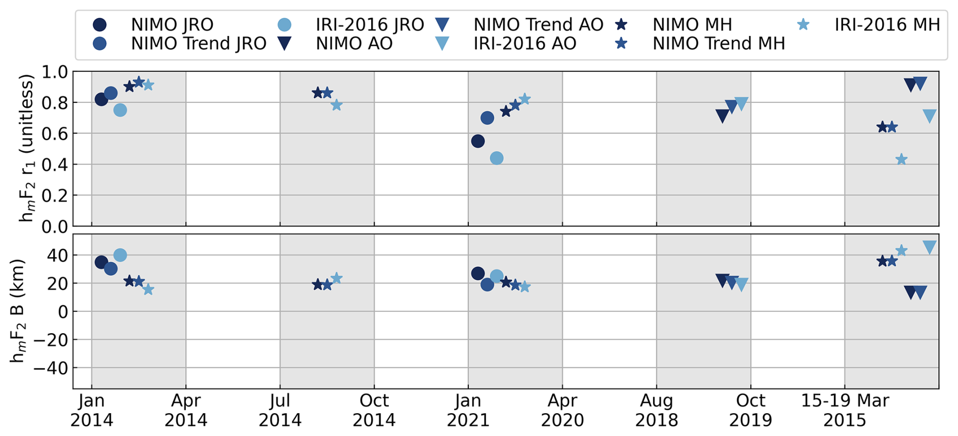
Figure 12 h_mF₂ r₁ (a) and B (b) for the JRO (circles), MH (stars), and AO (triangles) ISRs. The NIMO results are plotted in navy blue, the NIMO trend is plotted in slate blue, and the IRI-2016 results are plotted in light blue.

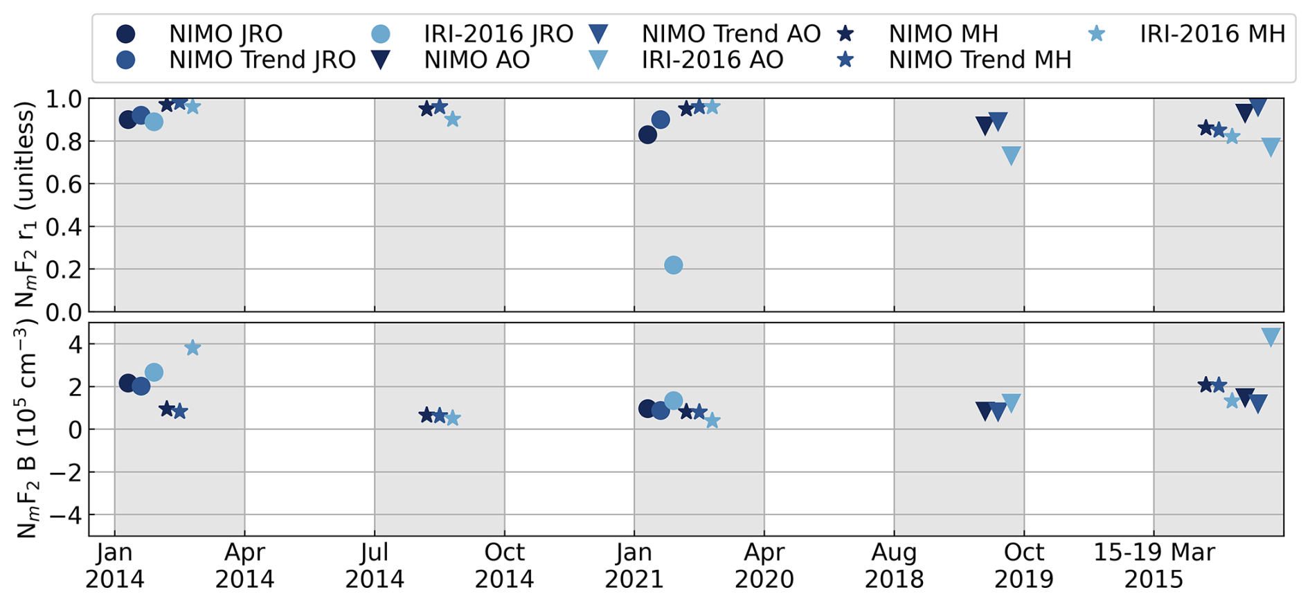
Figure 13 N_mF₂ r₁ (a) and B (b) for the JRO (circles), MH (stars), and AO (triangles) ISRs. The NIMO results are plotted in navy blue, the NIMO trend is plotted in slate blue, and the IRI-2016 results are plotted in light blue.

4.3.3 GNSS CONUS TEC

This section examines the GNSS VTEC from the Madrigal database over a validation region within the Contiguous United States (CONUS), shown with the green box in Fig. 5. This region was chosen for this validation because it is heavily instrumented. To facilitate analysis, the Madrigal TEC is linearly interpolated onto the NIMO TEC grid, reducing the resolution to 1° in latitude and 4° in longitude. The Madrigal data time step closest to each NIMO output time is retained for comparisons.

The Madrigal TEC is also compared to IRI-2016 TEC outputs. The IRI-2016 TEC is also linearly interpolated onto the NIMO TEC grid increasing the resolution to 1° in latitude and 4° in longitude. The Madrigal data time step closest to each IRI-2016 output time is retained for these comparisons.

The results of the Madrigal vertical TEC validation, presented in Table A5 and Fig. 14, show that NIMO typically outperforms IRI-2016, having a P_B=66.67 % and a P_RMSE=100 %. Both NIMO and IRI-2016 agree with the data better during the solar quiet periods than the solar active or storm periods.

Figure 14 CONUS TEC B (a) and RMSE (b) for all validation runs.

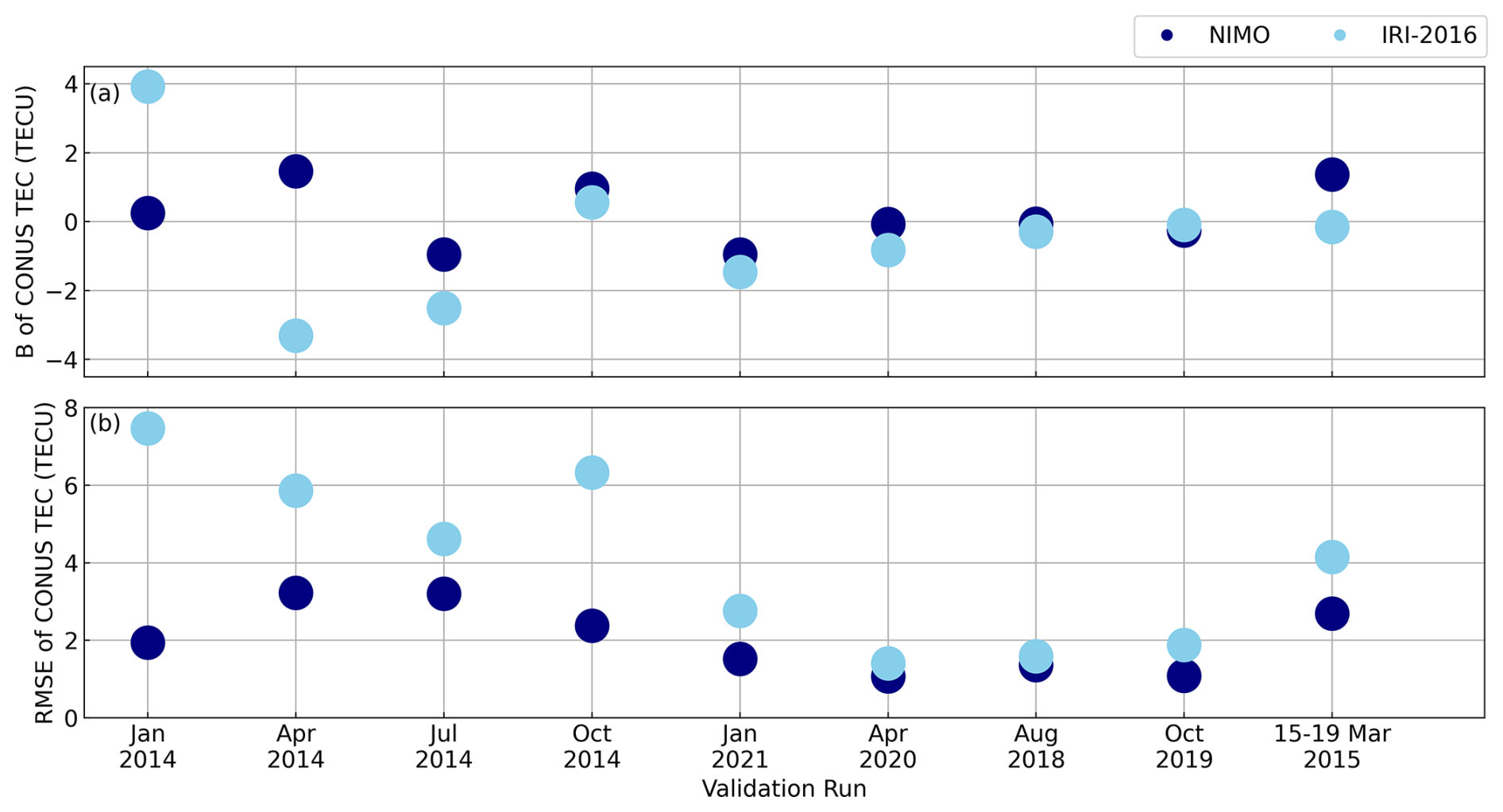
An example of the time evolution of these statistics is included in Fig. 15, which shows one of the time periods where the IRI-2016 B performs better than the NIMO B. The top left panel shows the average TEC within CONUS over the duration of the October 2014 run for both NIMO and Madrigal TEC. NIMO tracks the daily variation well but overshoots the daily maxima by a little bit during the latter half of the month. The generally good agreement is supported by the resulting small B and RMSE in the top right panel.

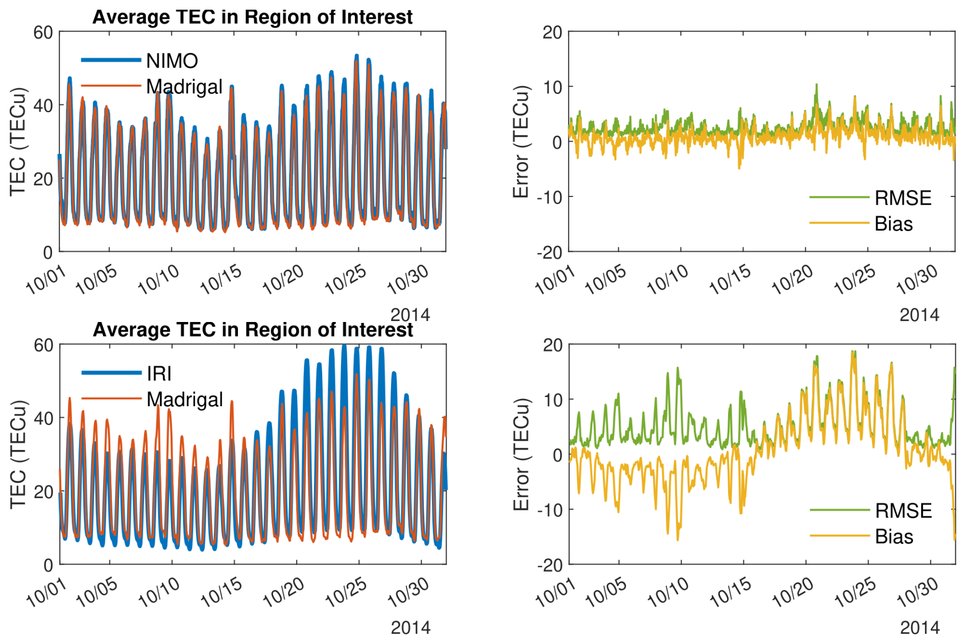
Figure 15 Time evolution of the average TEC in CONUS for NIMO, IRI-2016, and Madrigal TEC (left column) and the resulting statistics (right column) during the October 2014 run.

By comparison, IRI-2016 and Madrigal average TEC are shown in the bottom left panel. IRI-2016 typically undershoots the TEC for the first half of the month but significantly overshoots the daily maxima during the second half of the month. This tendency to both overestimate and underestimate the TEC in IRI-2016 is captured by the B trending negative during the first half of the month and then positive during the second half of the month. However, these opposing biases average out when considering the period as a whole. This causes the small B for the entire run, shown in Table A5, and highlights why the B must be considered alongside other metrics when evaluating model performance.

4.3.4 JASON TEC

The JASON-2 and JASON-3 altimeters provide direct measurements of the nadir TEC between the spacecraft (mean altitude of 1340 km) and the Earth's surface. The measurements are only available over the oceans (Fig. 16), but are a good complement to land-based GPS receiver measurements. With an inclination angle of 66°, each JASON satellite slowly precesses through all local times in ∼ 2 months; thus each validation month covers roughly half of the local times, as illustrated in Fig. 17 for January 2021. For more details on the JASON measurements, refer to Sect. 4.1.4 and references therein.

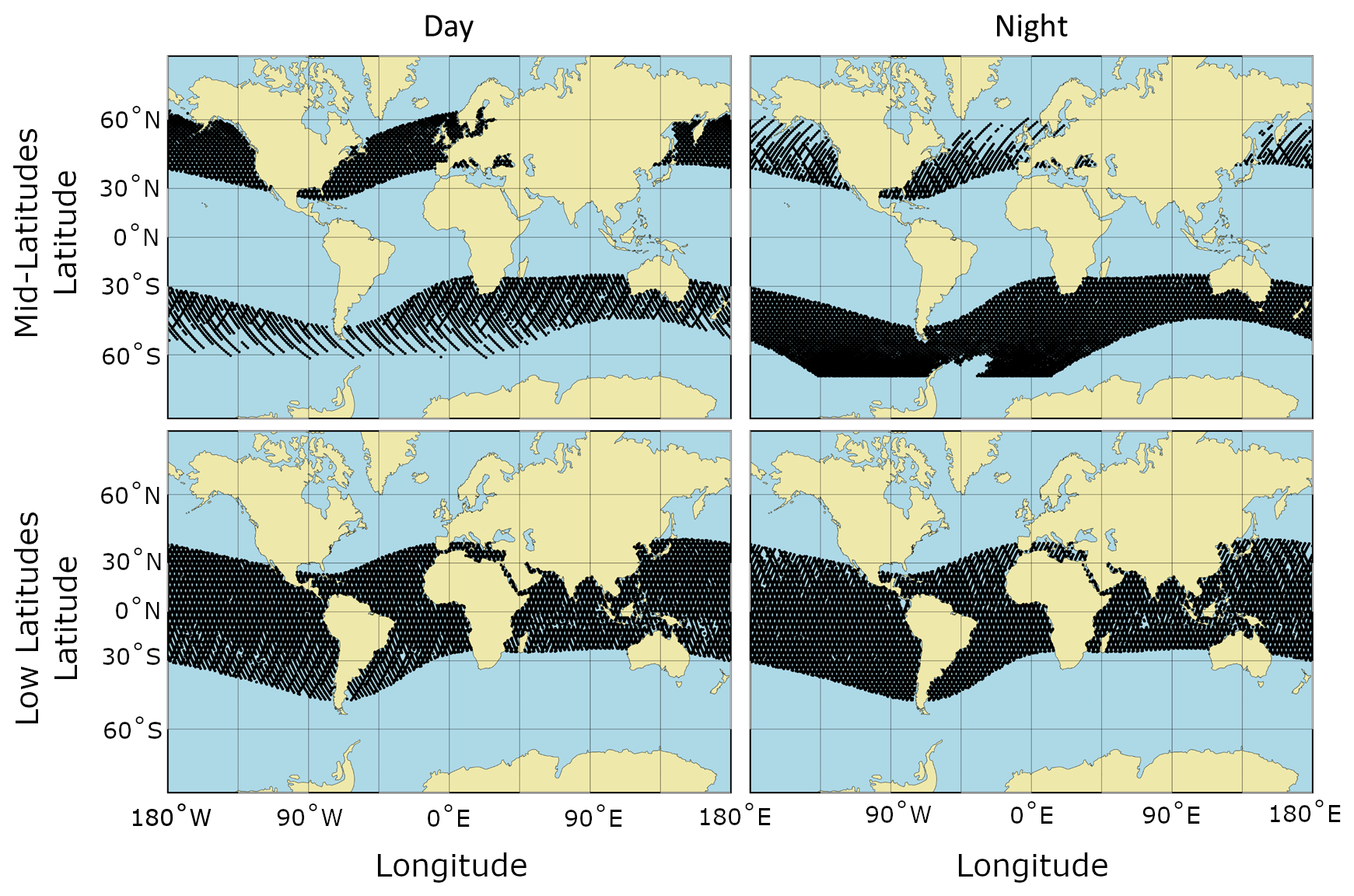
Figure 16 JASON-2 data coverage in January 2014 as a function of latitude and longitude for the mid- and low-latitudes at daytime and nighttime. For this report, we define mid-latitudes as latitudes between 60 and 35° north and south of the magnetic equator. Low-latitudes include regions within 35° of the magnetic equator. Daytime passes includes local times between 06:00 and 18:00 SLT, and nighttime passes are between 18:00 and 06:00 SLT.

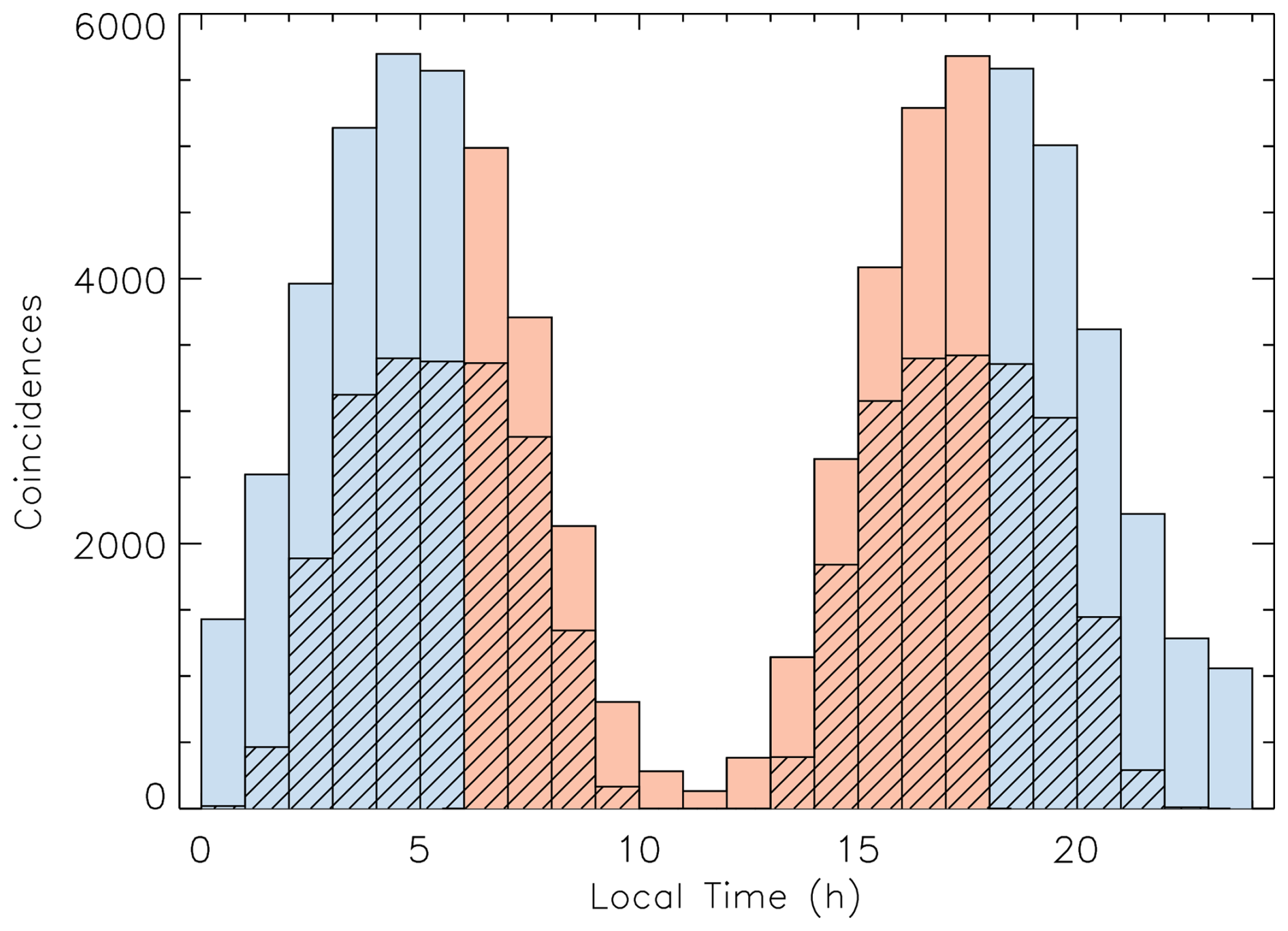
Figure 17 JASON-2 data coverage in January 2014 as a function of SLT. The blue bars indicate nighttime measurements, defined as the SLT between 18:00–06:00 SLT, and the red bars show the daytime measurements. Bars with diagonal lines show the portion of the measurements in the low-latitude region.

Overall, the validation shows that NIMO TEC, calculated up to 1340 km in altitude, compares well with JASON TEC measurements and outperforms IRI-2016. The global statistics for each validation run are shown in Table A6 and by the filled circles in Figure 18. Seasonal and solar cycle variations in the RMSE are highlighted in Fig. 19.

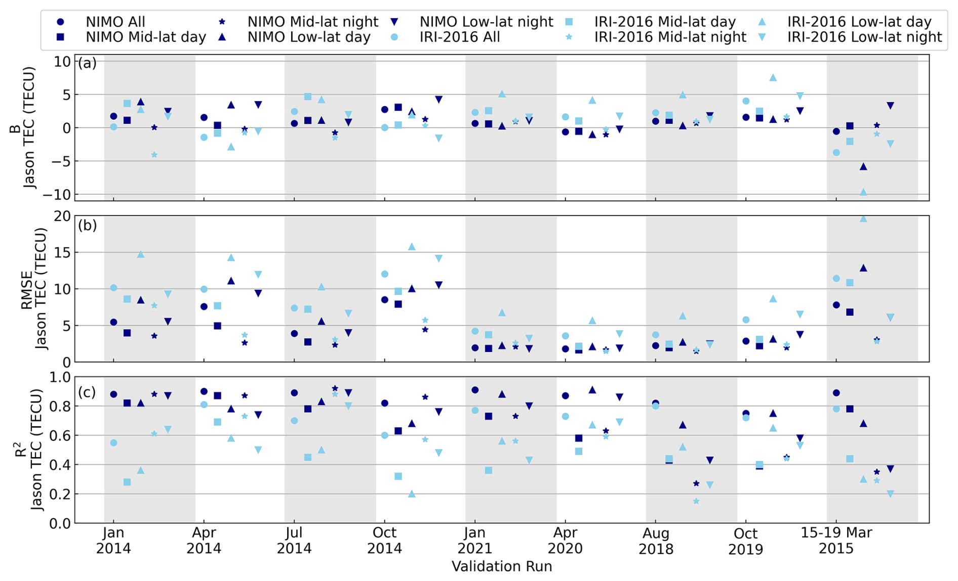
Figure 18 JASON TEC B (a), RMSE (b), and R² (c) for all validation runs, latitudes, and local times.

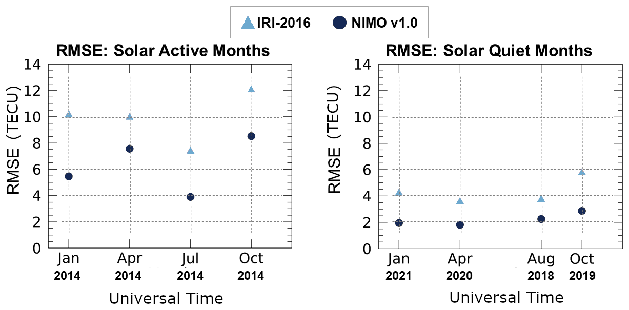
Figure 19 JASON RMSE for NIMO (black circles) and IRI-2016 (red triangles) over solar active and quiet validation runs.

During the solar active months in 2014, the NIMO RMSE was lower than that of IRI-2016 by 37 % and during solar quiet months the improvement is more than 40 %. Both models show a seasonal change in performance during the solar active runs that is not present during the solar quiet runs, with the solstices having lower RMSE values than the equinoxes. Additional metrics used for this analysis include the B and R² (see Sect. 4.2.2, 4.2.3, 4.2.7). The R² shows a higher correlation between the NIMO results and the data in all instances, while the B is typically lower in the NIMO results.

Breaking the data down into the four regions shown in Fig. 16 permits the validation of low-latitudes (within 35° of the magnetic equator) and mid-latitudes (between 60 and 35° north and south of the magnetic equator) in two local time regions that largely encompass day (06:00–18:00 SLT) and night (18:00–06:00 SLT) times, as was done for the ionosondes. The mid-latitude results are presented in Table A7 and shown in Fig. 18 by squares and stars. To summarize across all of the validation runs, the mid-latitude daytime results show NIMO has more realistic TEC values than IRI-2016 with $P_{R^{\mathrm{2}}}=\mathrm{77.78}\mathit{\%}$, P_B=88.89 % and P_RMSE=100 %. The mid-latitude nighttime results also show better agreement between NIMO and the JASON observations, with $P_{R^{\mathrm{2}}}=\mathrm{100}\mathit{\%}$, P_B=77.78 % and P_RMSE=77.78 %. In the low-latitudes (presented in Table A8 and shown in Fig. 18 by upward and downward facing triangles), all of the daytime and nighttime NIMO results correlate better with the JASON observations ($P_{R^{\mathrm{2}}}=\mathrm{100}\mathit{\%}$). The P_RMSE also shows NIMO doing a better job representing the observations than IRI-2016 in both local time groups, with values of 100% for the daytime and 88.89 % for the nighttime. The B comparison is weaker, with NIMO outperforming IRI-2016 in the daytime (P_B=66.67 %), but not at night (P_B=44.44 %). However, this can be explained by examining the different TEC distrubutions. An example of the type of distribution where IRI-2016 performs better than NIMO is shown in Fig. 20. The wider typical deviation between the IRI-2016 and JASON observations has a tendency to balance out, as reflected in the performance of the R² and RMSE statistics.

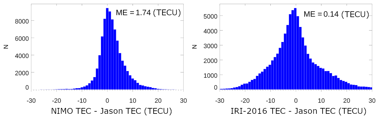
Figure 20 Difference histograms of the TEC between the models NIMO (left) and IRI-2016 (right) and JASON-2 in January 2014.

4.3.5 Topside Plasma Density

The topside ionosphere, the O⁺ dominated region above the F₂ peak, is dominated by plasma transport processes. In different latitudinal regions, the magnetic field structure leads to different types of interactions between the ionosphere, thermosphere, and magnetosphere. This validation uses in situ measurements of the plasma density from IVMs flown onboard the C/NOFS, DMSP, and ICON satellites. The data from the satellites are paired directly with the model output, reducing the number of samples available for the validation based on the model's 15 min cadence. This direct pairing was chosen to avoid introducing interpolation into the validation process and avoid considering structures with time-scales smaller than the model is capable of reproducing. For more details about these data sets, see Sect. 4.1.5, 4.1.6, and 4.1.7.

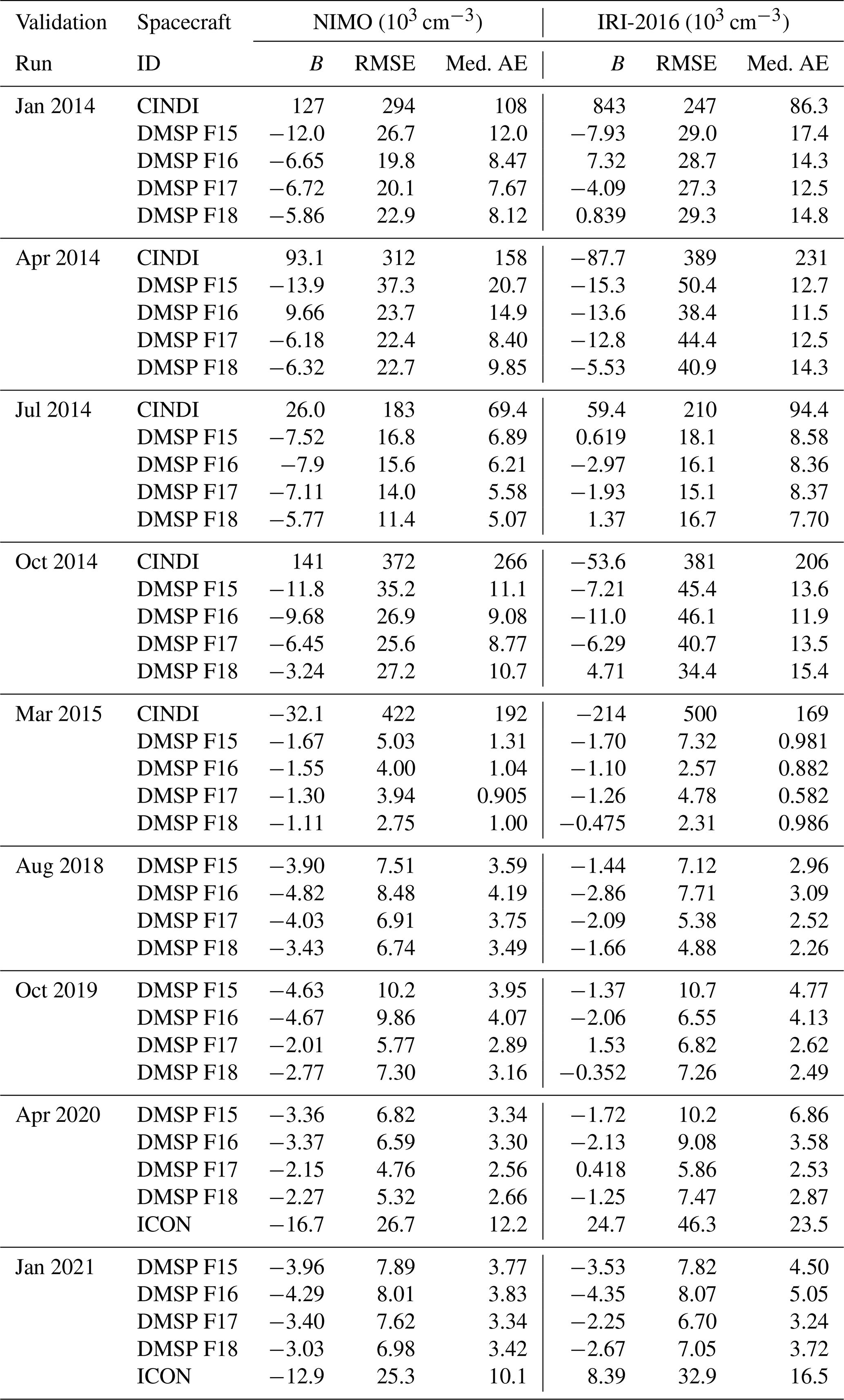
The results of the topside ionosphere validations, presented in Tables A9 and A10, may be summarized for all satellites and regions with NIMO outperforming IRI-2016 in the error meta analysis, but not the bias, with P_B=27.9 %, P_RMSE=74.4 %, and $P_{\mathrm{Med}.\mathrm{AE}}=\mathrm{62.8}\mathit{\%}$.

A more detailed look at the topside error is presented in Fig. 21, which presents the seasonal variations for each spacecraft used in the model validation for the solar active and solar quiet periods. The seasonal and solar cycle variations are similar to those seen by the JASON TEC in Fig. 19. During the solar active year of 2014 NIMO and IRI-2016 perform better during solstices than equinoxes, with the best performance seen during July 2014. During the solar quiet years, no seasonal variation is present, and both IRI-2016 and NIMO have lower Med. AE values then they do during the solar active years.

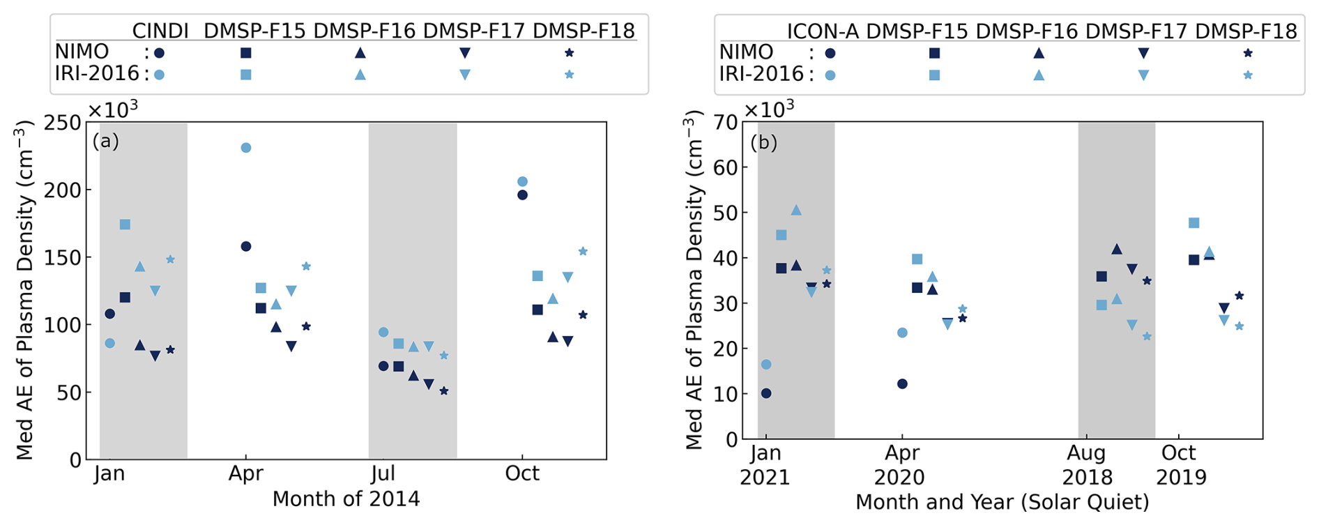
Figure 21 Med. AE of the different topside satellites (circles, squares, upward and downward triangles, and stars) compared to NIMO (navy blue) and IRI-2016 (light blue) over solar active (left, a) and quiet (right, b) validation runs. The shaded boxes mark the solstice seasons.

The DMSP results were further broken down into different local time regions that were chosen to encompass times with similar physical processes, four of which contained sufficient data to be used for model validation. These four groups, and the reason behind their selection are: 02:00–06:00 SLT contains sunrise, 06:00–08:00 SLT contains the morning hours at northern mid-latitudes (for F18, the only spacecraft to use this bin), 12:00–17:00 SLT contains the afternoon density peak, and 17:00–20:00 SLT contains sunset. The summary of these results is shown in Fig. 22. This figure shows that NIMO most consistently performs better than IRI-2016 during the 02:00–06:00 SLT period. During the other local time periods NIMO models the topside plasma density better than IRI-2016 during the solar active runs, but not during the solar quiet runs.

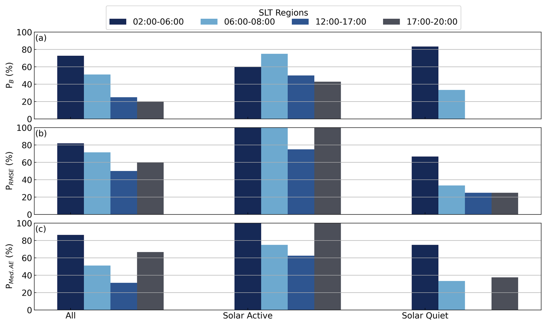
Figure 22 Percentage of runs for different SLT regions (differentiated by color) where NIMO outperforms IRI-2016 for DMSP F15-F18 considering P_B (a), P_RMSE (b), and P_Med.AE (c).

5 Conclusions

NIMO is a new operational, ionospheric model that brings together the expertise of the ab initio SAMI3 ionospheric model and IDA-4D data assimilation to provide hindcasts, nowcasts, and forecasts of the ionospheric electron density. NIMO v1.0 is the first stable version of this model, later versions of which have been transitioned for use in an operational environment. The validation of NIMO v1.0 demonstrates the combined ability of data assimilation and physics-based modeling to provide realistic calculations of electron density over the entire terrestrial ionosphere.

NIMO was extensively validated against a variety of available ionospheric data sets, with the goal of benchmarking its performance near and away from locations of assimilated data in the F region. As all models need to be validated against independent data sets, special emphasis is placed on the JRO ISR, JASON TEC, CINDI, DMSP, and ICON observations. These data sets were not used in the data assimilation nor are they reliant on any potentially assimilated data (the AO ISR uses ionosonde data to assist in the altitude calibration).

The ionosonde validation showed no consistent local time variations in the relative performance of the two models. It found that NIMO performed better than IRI-2016 when modeling the f_oF₂, while IRI-2016 did slightly better at modeling the h_mF₂. The only exception is times with geomagnetic storms, where NIMO consistently modeled the F₂ peak characteristics better than IRI-2016. In Fig. 7 at around 01:30 UT the model matches an unrealistic h_mF₂. This problem comes from how the ionosonde data is quality controlled and how IDA4D assimilates the data. Work is ongoing to improve cleaning of ingested data and how the data assimilation system handles outlier data.

The ISR validation was able to examine portions of five of the nine desired validation periods at either AO, JRO, or MH (with some overlap in the time periods). At all times and locations, NIMO provided a more accurate specification of the electron density than IRI-2016 and the NIMO climatological trend slightly outperformed the standard NIMO output. This shows that while NIMO does a good job representing the N_mF₂ and h_mF₂ at mid-, low-, and equatorial latitudes, the small-scale variations do not exactly match those seen in the observations. This is an area of improvement to address in future model releases.

The CONUS GNSS TEC validation found that NIMO continued to outperform IRI-2016, with the RMSE reflecting NIMO's ability to capture day-to-day variations in the VTEC over each validation period. Both the B and RMSE showed that NIMO performed better in the CONUS region of interest at solar quiet times, with the solar active periods and the storm validation run having similarly worse RMSE values.

The JASON TEC validation focused on the model performance over the oceans, where the amount of data contributing to assimilation or the formation of an empirical model is low. It found that NIMO better represented the TEC over the oceans than IRI-2016 in all the validation runs. This performance was consistent when looking at the global picture or narrowing the focus to smaller latitudinal and local time regions.

The CINDI, DMSP, and ICON validation focused on the model performance in the topside ionosphere. It found that NIMO fared better than IRI-2016 during solar active periods, though both NIMO and IRI-2016 had smaller errors during solar quiet periods. The topside ionospheric validation showed seasonal variations in the Med. AE that were similar to those seen in the JASON TEC RMSE.

The storm time response from NIMO was also more representative of the ionosphere across all validation sets, when compared against IRI-2016. Examining just the RMSE from data containing all local times, P_RMSE for the Mar 2015 storm was 60 %. The ISR runs (which did not use RMSE) had $P_{r_{\mathrm{1}},B}=\mathrm{75}$ % against the unaltered NIMO output.

The results of this validation demonstrate that the current capabilities to specify the electron density using NIMO v1.0 are as good or better than climatology, as provided by IRI-2016. Particular improvement is seen over the oceans, where data assimilation and data-based climatologies are less able to provide constraints. Future versions of NIMO will include improvements to the data assimilation and physics-based processes, aiming to improve the regions that this validation revealed as weaknesses. These future versions of NIMO and other ionospheric models may compare their electron density specifications against the results presented here. The metrics that provide the greatest utility across multiple model validations may then be considered as standard validation metrics in the ionospheric community as a common scorecard is developed, such as the scoreboards for solar flares or sudden energetic particles provided by the NASA Community Coordinated Modeling Center. Future validation efforts may also include a wider range of metrics that capture the variations in the bottomside ionosphere, as well as the morphology of key features like the Equatorial Ionization Anomaly.

Appendix A

Statistics from each of the different instrument comparisons discussed in Sect. 4.3 are presented here in a tabular form. By providing the values of the statistics for each data-model comparison, future validations can use these results in an apples-to-apples benchmarking.

Table A1 Global f_oF₂ statistics in different local time bins for all ionosonde locations.

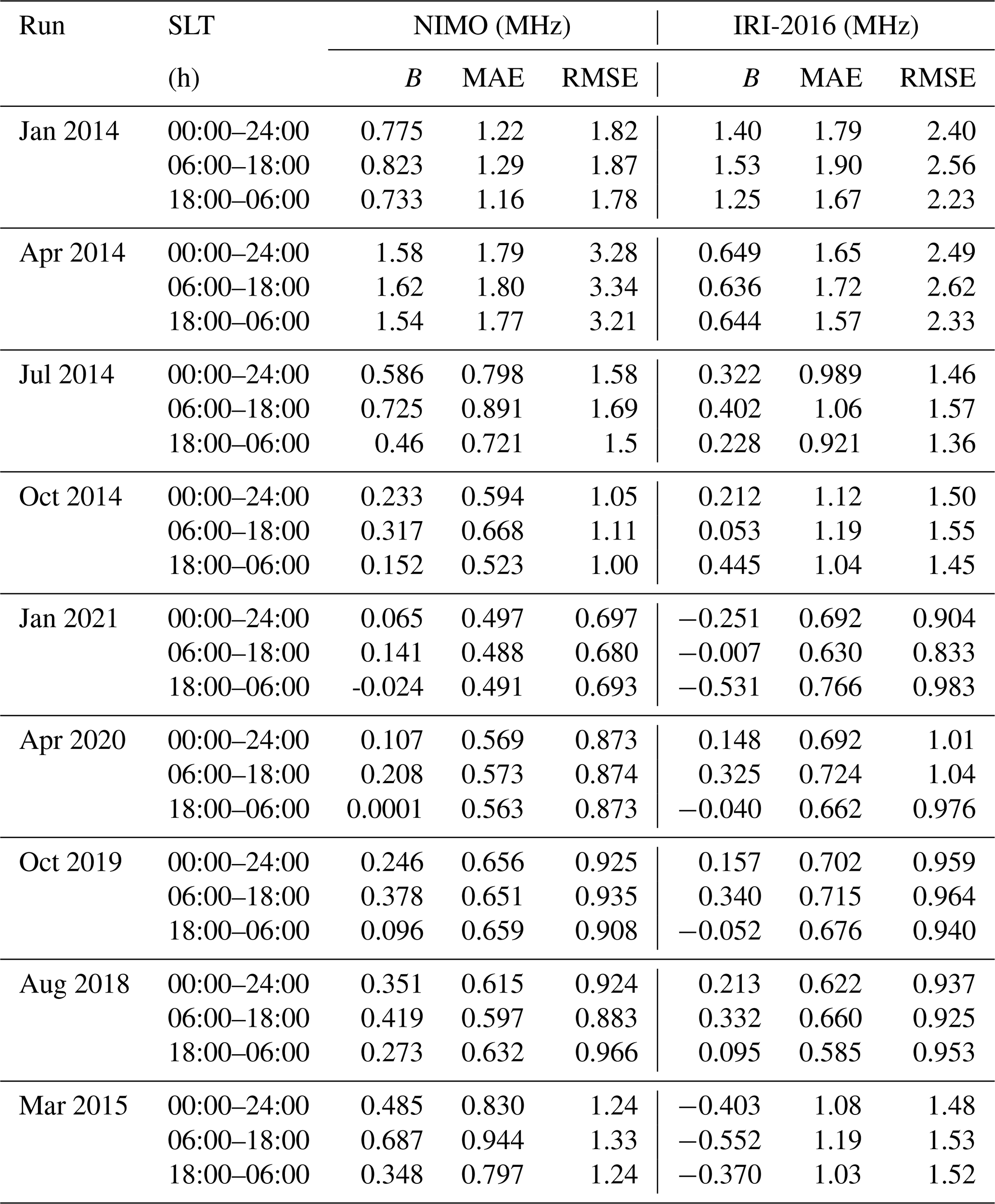
Table A2 Global h_mF₂ statistics in different local time bins for all ionosonde locations.

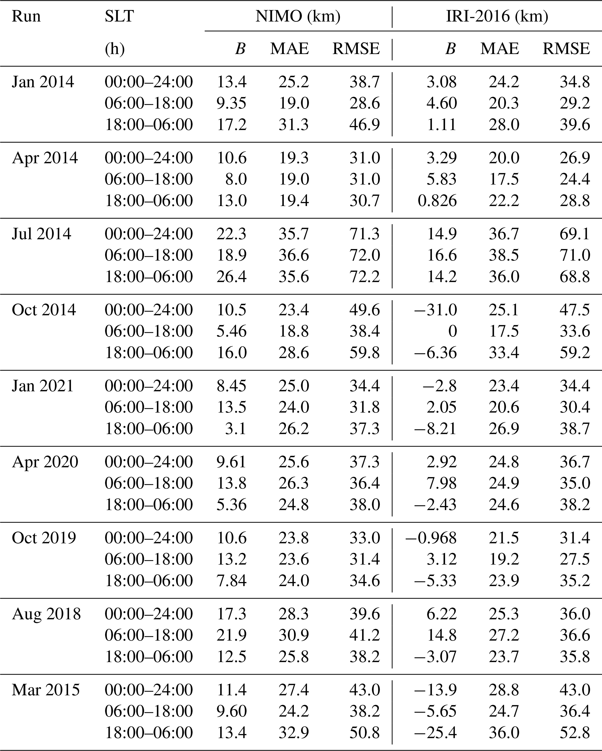
Table A3 NIMO trends and IRI-2016 correlation factor (r₁) with the ISR data for h_mF₂ at the ISR locations.

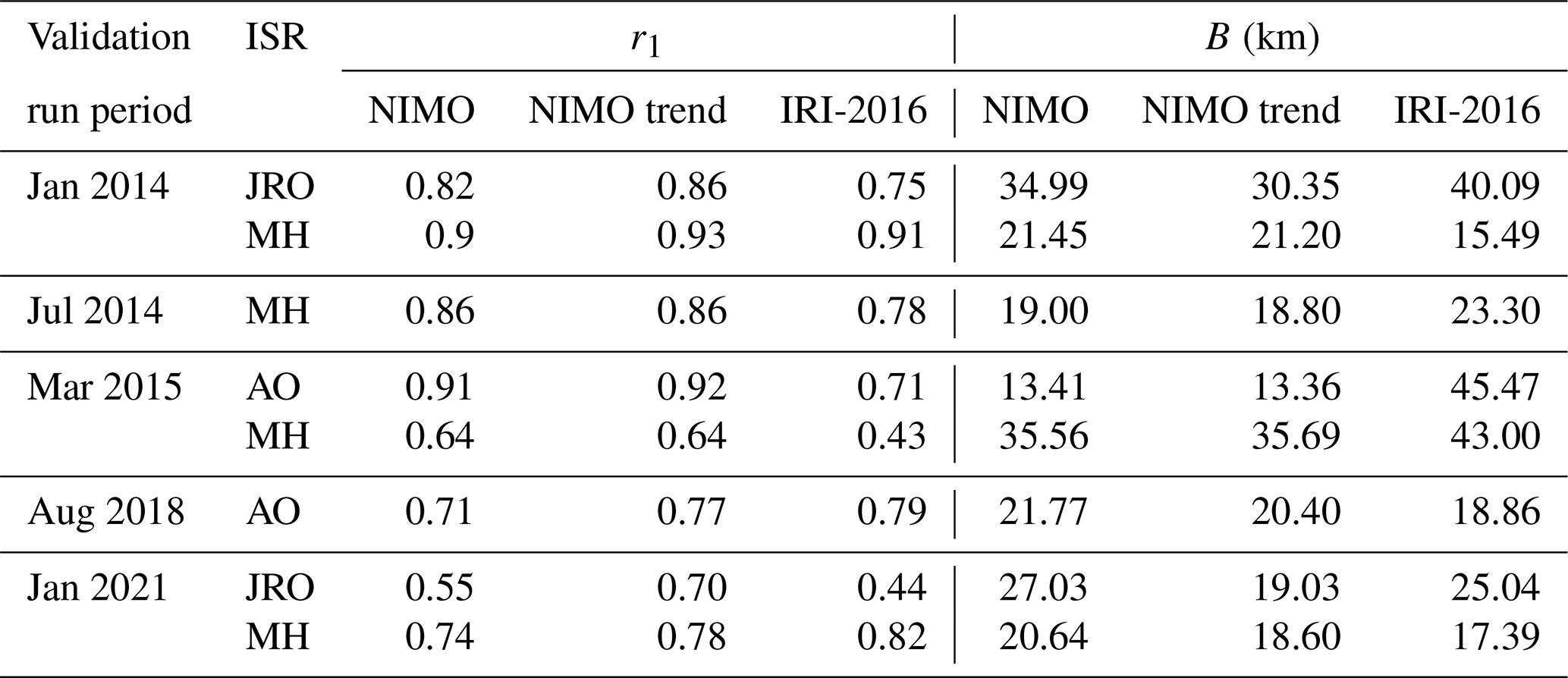
Table A4 NIMO trends and IRI-2016 correlation factor (r₁) with the ISR data for N_mF₂ at the ISR locations.

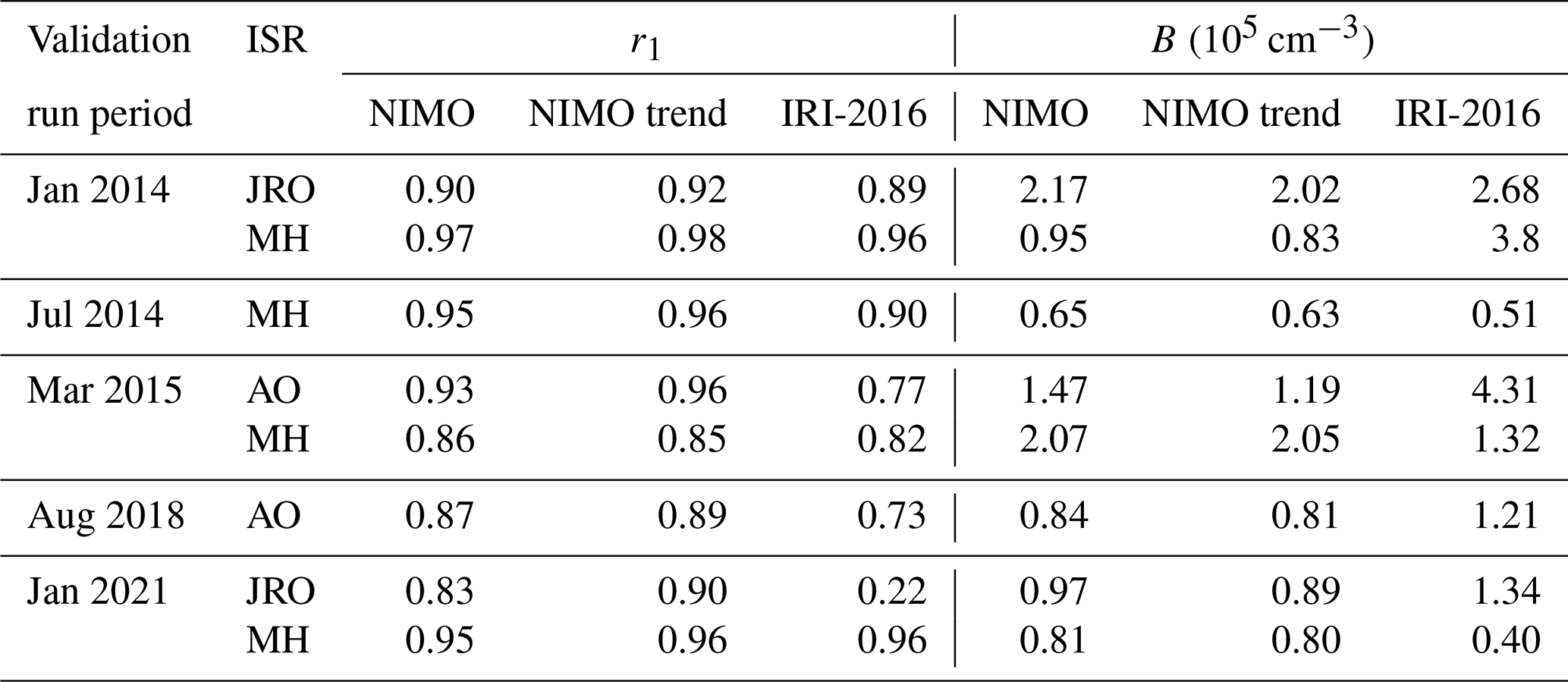
Table A5 Vertical TEC statistics from CONUS during solar active conditions.

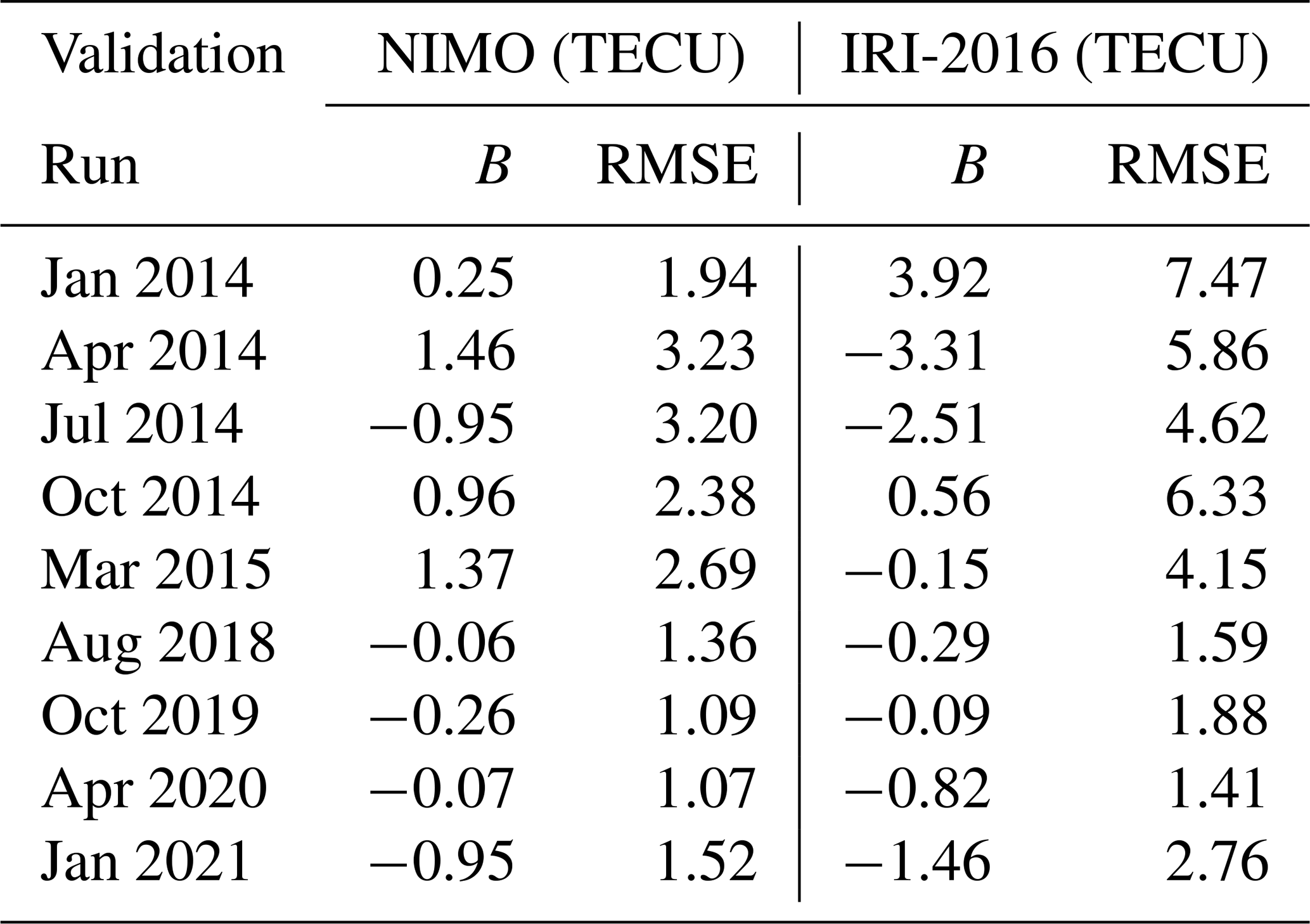
Table A6 Global TEC statistics from JASON-2 for all local times.

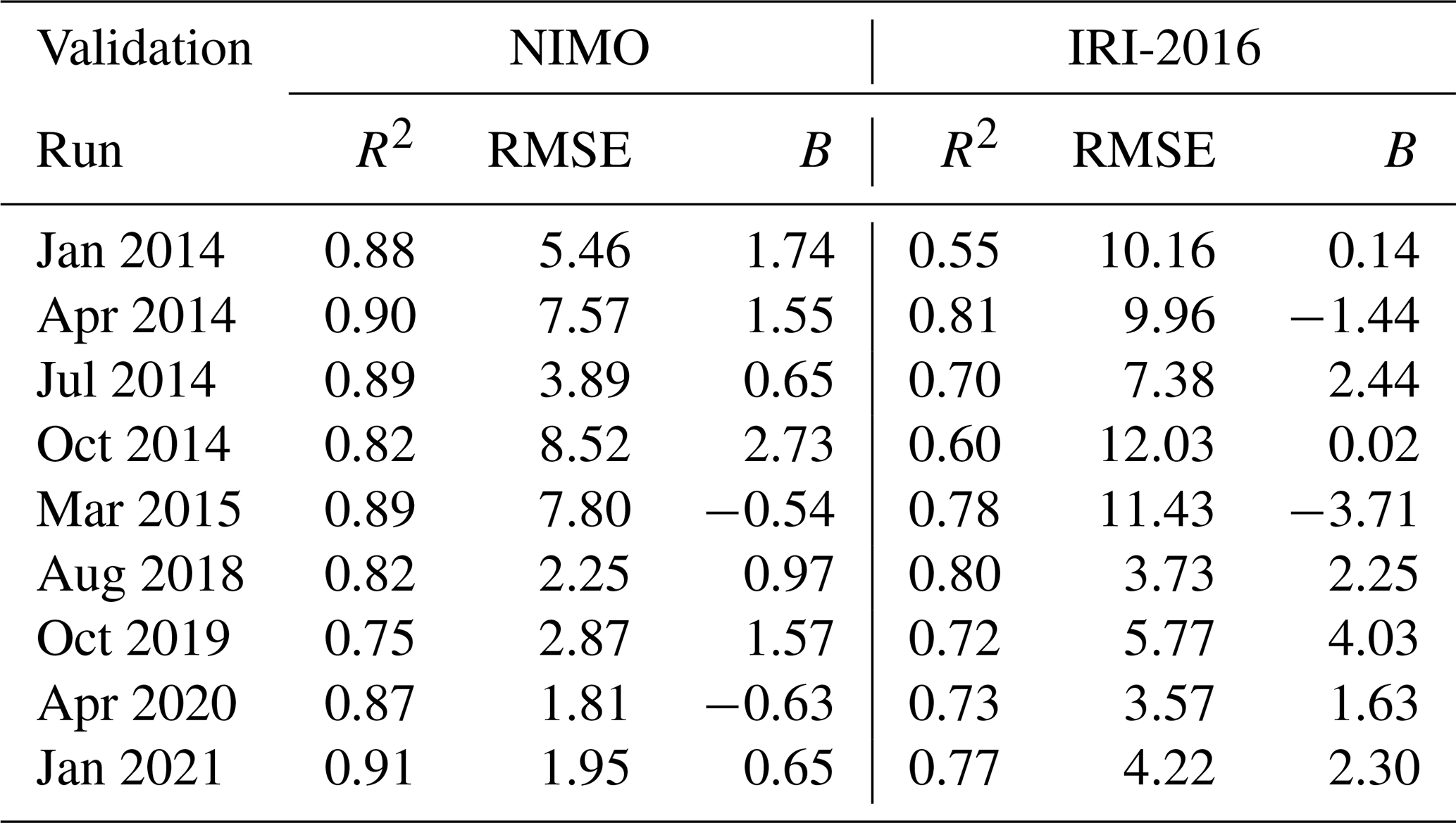
Table A7 Mid-latitude TEC statistics from JASON-2 for day and night times.

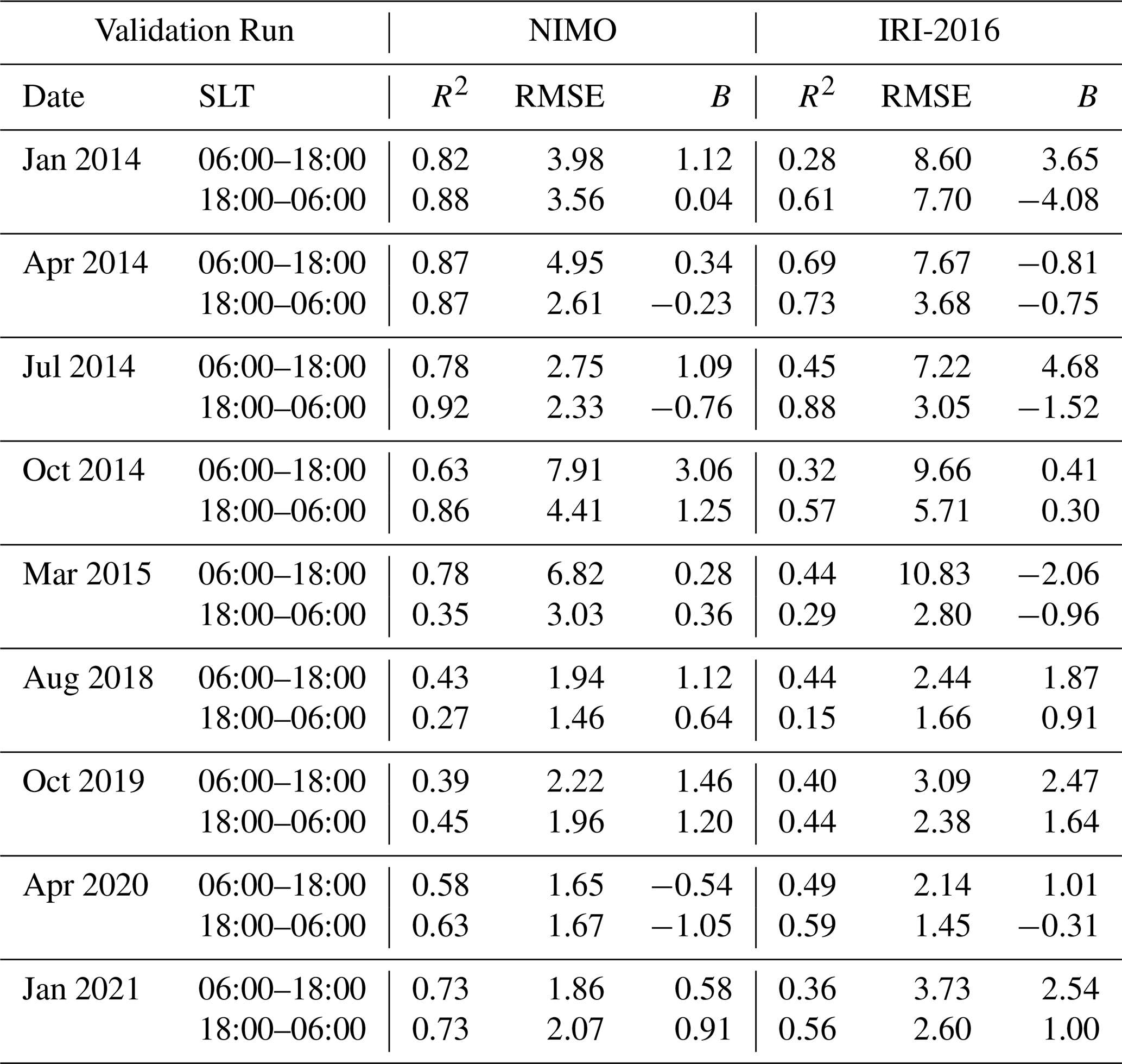
Table A8 Low-latitude TEC statistics from JASON-2 for day and night times.

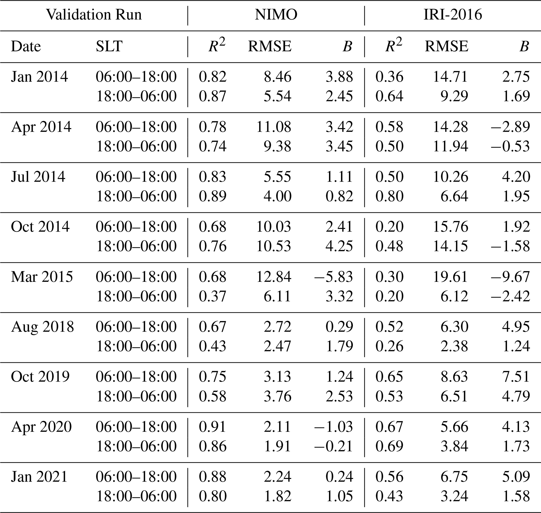
Table A9 Global, topside ionosphere statistics from DMSP for SLT regions.

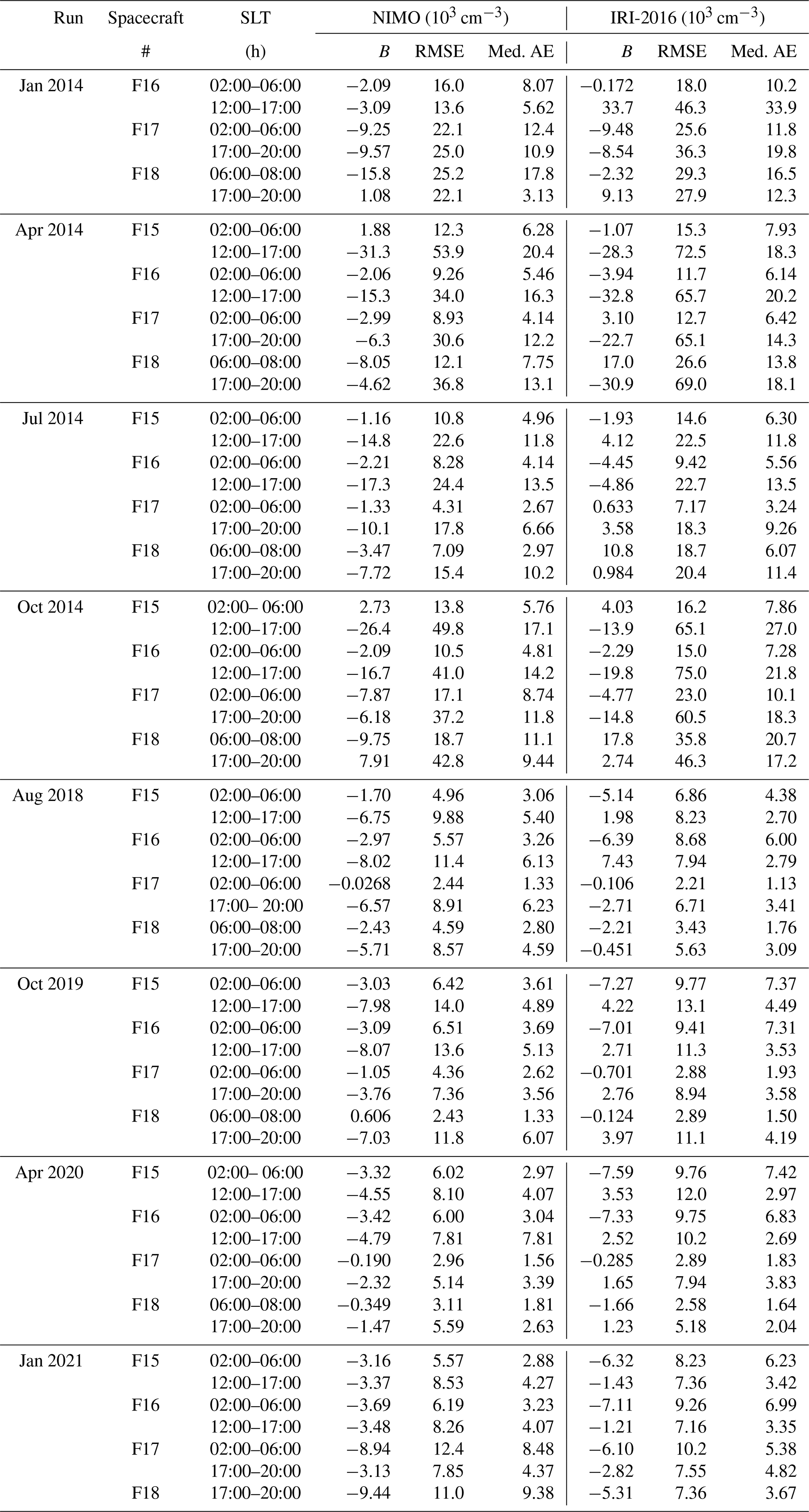
Table A10 Global, topside ionosphere statistics from CINDI, DMSP, and ICON for all local times.