Benchmarking the Swedish Power Grid Against a 1-in-100-Year Geoelectric Field Scenario

Sweden’s communication and power systems have been impacted by major space weather events in the past. For instance, the May 1921 storm caused a fire at the telegraph and telephone station in Karlstad, and the 2003 Halloween storm led to a blackout in Malmö. In this study, we present the first comprehensive assessment of the potential impacts of a 1-in-100-year extreme geoelectric field on the entire Swedish power grid. Using magnetic field observations from the 30 October 2003 event as a baseline, we constructed two extreme scenarios. In Case 1, we used the observed magnetic field across Fennoscandia. In Case 2, we assume an idealized ionospheric current system in which all stations share the same temporal magnetic field pattern. Then the estimated 3D geoelectric field was scaled using region-specific scaling factors derived from recent statistical analyses of geoelectric field extremes in Sweden. The scaled geoelectric field and power line voltages are computed using the recently developed RAISE model, which includes realistic ground conductivity and power line topology. Our results show that the largest-magnitude horizontal geoelectric fields, around 12 V km⁻¹, occur within the 55 and 58° MLAT band, particularly in regions with sharp lateral conductivity gradients. East–west-oriented power lines are especially vulnerable, as they are mainly located south of 60° MLAT, where the largest geoelectric fields are calculated. Overall, during the peak of a 1-in-100-year geomagnetic storm, more than 100 transmission lines are expected to experience voltages above 50 V multiple times over the course of the substorm. At the peak of the largest disturbance, triggered by a sudden weakening of the westward electrojet, around 100 lines are expected to exceed 100 V. These results provide critical insights into infrastructure vulnerability under extreme space weather conditions.

1 Introduction

The vulnerability of modern infrastructure to major space weather events is an increasing concern, given society’s growing dependence on reliable electrical and communication systems. Power transmission grids are particularly at risk from geomagnetically induced currents (GICs), which are driven by rapid variations in the geomagnetic field during geomagnetic storms. These currents can disrupt normal grid operations and, in the worst cases, cause permanent transformer damage or trigger widespread, unnecessary tripping of both power lines and transformers, potentially resulting in large-scale power outages (e.g., Bolduc, 2002; Pulkkinen et al., 2005; Girgis and Vedante, 2012). While ground magnetic field perturbations ($\mathrm{d}B/\mathrm{d}t$) are often used as proxies for GIC activity (Viljanen et al., 2001), the horizontal geoelectric field (E_H) is a more direct and physically meaningful driver, as it incorporates the effects of local ground conductivity (Pulkkinen et al., 2017). Consequently, several statistical studies have examined high-amplitude geoelectric field values in different areas, including Canada (Cordell et al., 2025), Ireland (Malone-Leigh et al., 2024), and Sweden (Lanabere et al., 2023, 2024). Although extreme events are typically low-probability but high-impact, it remains essential to define what constitutes an extreme event in order to benchmark worst-case scenarios.

A worst-case scenario is typically defined as an event with an occurrence rate of 1-in-100 years (Pulkkinen et al., 2012). In this paper, we use the term extreme exclusively for 1-in-100-year events. All other impactful events (e.g., strong, intense, or severe) are referred to as major events. The global level of geomagnetic activity is commonly quantified using the Dst index. The largest Dst depression inferred to date is associated with the Carrington event (Carrington, 1859), with estimates ranging from approximately −850 to −1760 nT (Tsurutani et al., 2003; Siscoe et al., 2006). Although the exact recurrence rate of such a high-magnitude event remains uncertain, recent statistical analyses suggest a return period on the order of 1000 years, with confidence intervals ranging from approximately 400 to 2800 years (Love et al., 2024). Another event exceeding the 1-in-100 year threshold was the May 1921 storm, with an estimated Dst of about −900 nT (Kappenman, 2006; Hapgood, 2019). The next largest event was the March 1989 storm (Dst ∼ −589 nT), which has an estimated occurrence rate of about 1 in 60 years (Tsubouchi and Omura, 2007) to 1 in 100 years according to Bergin et al. (2023). However, these earlier events were poorly documented due to limited observational coverage at the time. The first well-recorded major geomagnetic storm was the Halloween event of 29–30 October 2003, which reached a minimum Dst of approximately −400 nT. More recently, the major storm of 10–12 May 2024 reached a minimum Dst of about −412 nT, making it the largest geomagnetic storm since the Halloween storms of 2003 and the second largest event after the 13 March 1989 storm.

Previous worst-case studies have used the records of the latest geomagnetic storms to reconstruct 1-in-100 years scenarios for the geoelectric field event (Pulkkinen et al., 2012; Ngwira et al., 2013). Other studies, however, have adopted alternative approaches by scaling the geomagnetic field (NERC, 2016, the North American Electric Reliability Corporation), and the magnetic field perturbation (Mac Manus et al., 2022) into a 1-in-100 years scenarios. In order to scale the geoelectric field, magnetic field, or its perturbation, the mentioned authors have used different scaling methods to account for the maximum intensity and return values dependence with magnetic latitude (MLAT). Then, the MLAT threshold of the extreme events becomes an important factor. For instance, Pulkkinen et al. (2012) analyzed two major geomagnetic storms, and proposed that the maximum disturbances typically occur near 50° MLAT. Later, Ngwira et al. (2013) extended the study to twelve major geomagnetic storm events and found that the latitude threshold boundary tends to occur between 50 and 55° MLAT. Regionally, Thomson et al. (2011) analyzed 28 years of European geomagnetic data and observed a local maximum around 53–62° MLAT for the time derivative of the horizontal magnetic field. This result is consistent with the findings of Lanabere et al. (2023), who showed that 58.7° MLAT had the highest frequency of the 15 largest events observed between 2000 and 2018. Additionally, the largest geoelectric field values in Sweden are expected to occur around 56.9° MLAT, according to (Lanabere et al., 2024).

The first worst-case scenario study for Sweden was conducted by Rosenqvist et al. (2022), who analyzed the ground magnetic response to a modeled “perfect” storm. Due to the current models limitations to fully capture the complexity of substorm dynamics, Rosenqvist et al. (2022) focused their analysis on magnetic field variations during the sudden impulse phase to predict a worst-case GIC magnitude for a power line in southern Sweden. However, large amplitudes $\mathrm{d}B/\mathrm{d}t$ are typically attributed to substorms at high latitudes (Viljanen et al., 2006; Kataoka and Ngwira, 2016) which are responsible for the largest E_H values estimated in Sweden (Lanabere et al., 2023). Thus, the impact of a 1-in-100-year event, associated with nightside events on Sweden’s power grid remains largely uncertain.

This paper extends the work of Rosenqvist et al. (2022) by analyzing ground magnetic data during the development of a premidnight substorm event. Following the approach of Pulkkinen et al. (2012), we define an extreme, or worst-case, event as the 100-year maximum amplitude of the E_H at 10 s resolution. The remainder of this paper is organized as follows. Section 2 describes the geomagnetic field data, the GIC-SMAP model developed by Rosenqvist and Hall (2019) to estimate the geoelectric field in Sweden, and the RAISE model (Rosenqvist et al., 2025), used to simulate the resulting power line voltages in the Swedish power grid under the scaled geoelectric field. In Sect. 3, we describe the selection of geomagnetic field observations from a past storm, and the application of scaling factors from Lanabere et al. (2024) to represent a 1-in-100-year event. In Sect. 4, we evaluate the impacts of the scaled geoelectric field on the power grid. Finally, Sects. 5 and 6 presents the discussion and conclusions respectively.

2 Data and models

2.1 Ground-Based Magnetometers

We used 10 s geomagnetic field data from the IMAGE (International Monitor for Auroral Geomagnetic Effects) magnetometer network. At the time of the Halloween storm in October 2003, 26 magnetometers were operational in the Fennoscandian region. The IMAGE magnetometer network has been used to compute the equivalent ionospheric currents, which represent the horizontal ionospheric currents that would be required to produce the observed ground magnetic variations (Amm, 1997). This approach is used to obtain the magnetic field all over Sweden. Moreover, since ground-based geomagnetic measurements include both external component (B_ext) produced by ionospheric and magnetospheric currents, and internal component (B_int) produced by induced telluric currents, the method has been further refined to separate these components, as described by Juusola et al. (2020). We refer the reader to Amm (1997) and Amm and Viljanen (1999) for a more detailed explanation of the ionospheric equivalent current technique and its applications.

2.2 The GIC-SMAP model

The GIC-SMAP model calculates the horizontal geoelectric field ${\mathbf{E}}_{\mathrm{H}}\left(\mathit{\omega }\right)=Z\left(\mathit{\omega }\right){\mathit{\mu }}_{\mathrm{0}}^{-\mathrm{1}}{\mathit{B}}_{\mathrm{H}}\left(\mathit{\omega }\right)$ in the frequency domain by relating the ground impedance tensor Z(ω) to local magnetic field perturbations B_H(ω). An inverse Fourier transform is then applied in order to transform into the time domain. In a new version of the model, where the E_H is computed at every point of the grid in Sweden, the magnetic field data is first interpolated using the Spherical Elementary Current System (SECS) method (Amm and Viljanen, 1999) using all available IMAGE stations.

The ground impedance tensor was previously obtained by computing the geoelectric field using a uniform magnetic field variation with unit amplitude, by solving the equations describing the current distribution in the ground in the frequency domain using the commercial software COMSOL Multiphysics for a unit-amplitude (H₀=1 A m⁻¹), uniform magnetic source field applied at 100 km altitude for a fixed set of frequencies (1–100 mHz). For further description of the COMSOL technical setup, see the supporting information (S2) in Dimmock et al. (2019) and Rosenqvist and Hall (2019) for additional details about the model.

The main source of uncertainty in the GIC-SMAP model arises from the sparse distribution of active IMAGE magnetometers in Sweden used in the SECS method to interpolate the magnetic field onto the model grid. Additional sources of uncertainty arise from the conductivity model (Marshalko et al., 2023). First, the underlying crustal conductivity map for the Fennoscandian Shield (SMAP) (Engels et al., 2002; Korja et al., 2002) is well constrained by extensive magnetotelluric surveys in northern Sweden, whereas large parts of southern Sweden remain sparsely surveyed and rely more heavily on extrapolated conductivity estimates. Second, the calculation of the surface impedance assumes a uniform magnetic field, whereas in reality, the magnetic field exhibits spatial variability. Third, frequencies below 1 mHz may contribute to the amplitude of the geoelectric field when superimposed on the higher frequencies (Wallner et al., 2026).

The model has been validated against GIC measurements in both northern and southern Sweden (Rosenqvist and Hall, 2019; Rosenqvist et al., 2022), indicating that the uniform-source-field assumption performs well during geomagnetically quiet periods, while further validation during geomagnetically active intervals remains pending.

2.3 The RAISE model

The recently developed RAISE model (Rymdvädersmodell för Analys av Inducerade Strömmar och Elektriska fält, Swedish for “Space Weather Model for the Analysis of Induced Currents and Electric Fields”), introduced by Rosenqvist et al. (2025), was employed to analyze the voltages in the Swedish power grid lines. The simplified Swedish power grid representation consists of 194 nodes and 335 transmission lines, of which 49 % are 400 kV lines and 51 % are 220 kV lines. This model has previously been applied to investigate GIC activity during the April 2023 and May 2024 geomagnetic storms (Dimmock et al., 2024; Rosenqvist et al., 2025). RAISE integrates the GIC-SMAP model (Rosenqvist and Hall, 2019) with a simplified representation of the Swedish high-voltage power grid, assuming constant earthing resistance and fixed line resistances for both 200 and 400 kV transmission lines. Due to this simplification in line resistances, the results presented here focus on calculated voltages without explicitly computing the corresponding GICs.

The RAISE model relies on the following assumptions and simplifications:

• Only transmission lines and power stations operated by the Swedish authority responsible for the electrical transmission system, Svenska Kraftnät (SvK), are included. Substations and lines owned by regional or private operators are not part of the dataset.

• Power Stations without verifiable connections are removed. Thus, power stations located more than 650 m from any mapped transmission line are excluded to ensure a topologically consistent network.

• International interconnections are omitted. This implies that all AC and DC links to neighboring countries (Norway, Finland, Denmark, Poland, Lithuania) are removed, and Sweden is treated as an electrically isolated system.

• The curvature of Earth is neglected, assuming that the distance between the nodes of the transmission line is of the order of hundreds of kilometers, much less than the Earth radius.

• The earthing resistance is considered constant, and the transmission lines are assumed to have a constant resistance per unit length depending on the transmission voltage level.

3 Method for defining worst-case scenarios

In this study, we follow the approach of Pulkkinen et al. (2012), defining a worst-case scenario when the amplitude of the E_H reaches a level that occurs once in 100 years. Our motivation for scaling the geoelectric field was that it is the physical driver of GICs. Using real ground magnetic perturbations as input preserves a realistic ionospheric forcing (rather than relying on a synthetic magnetic field time series), while the scaling ensures that the resulting geoelectric field reaches the level associated with a 1-in-100-year event from the perspective of the physical driver of GICs. This allows us to generate as many worst-case scenarios as magnetic field inputs are available. However, because ground magnetic perturbations are driven by ionospheric current systems that activate during geomagnetic storms and substorms, we recommend using magnetic field inputs from previously recorded events that produced the largest geoelectric field response.

To illustrate the range of possible worst-case conditions, we explore two complementary approaches. The first worst-case scenario (Case 1) is intended to remain as realistic as possible, with each geographic location experiencing a different magnetic field perturbation. This is achieved by using as many magnetometers as are available in Sweden, providing a well-resolved ionospheric driver. The second worst-case scenario (Case 2) is intended to represent an idealised case in which every location in Sweden experiences the same magnetic field perturbation (i.e., the frequency content remains identical). This is achieved by using data from a single magnetometer. Such an idealised situation could be produced by a large-scale westward electrojet (WEJ) extending across Fennoscandia.

Table 1 summarises the workflow of the analysis conducted in this study. Each step, from the selection of a previously observed event, the magnetic field inputs, the recreation of a 1-in-100-year E_H event, to the impact on the Swedish power grid, is listed along with the corresponding model and/or reference to previous studies.

Lanabere et al. (2023)Lanabere et al. (2024)Rosenqvist et al. (2025)Rosenqvist and Hall (2019)Lanabere et al. (2024)Rosenqvist et al. (2025)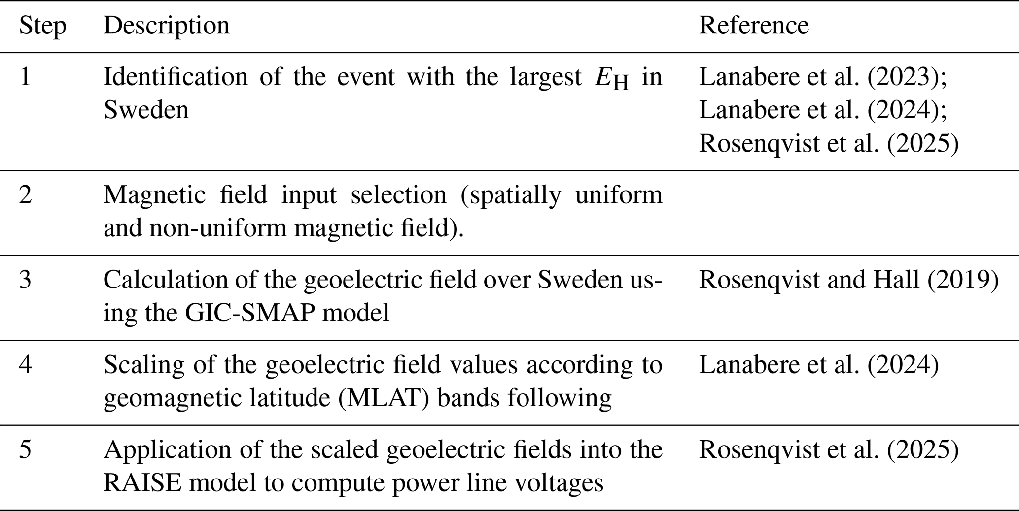

Table 1 Workflow of the analysis steps used in this study.

In the first step, we identified a past event with the largest E_H in Sweden, and that has been well-recorded. In a previous study, Lanabere et al. (2023) identified the event on 30 October 2003 at 20:03:40 ± 1 hour as the event producing the largest geoelectric field in Sweden during the last two solar cycles when derived using a 1D ground conductivity model (E_H=2.73 V km⁻¹). This result was later confirmed by Rosenqvist et al. (2025), who reported the largest geoelectric field derived using a 3D ground conductivity model (E_H=22.4 V km⁻¹) for the same event over the same period. The significantly higher value in Rosenqvist et al. (2025) is attributed to the fact that the maximum was observed near Sweden’s west coast, an area not covered in the analysis by Lanabere et al. (2023), and to the expected higher geoelectric field amplitudes from 3-D modelling compared with 1-D modelling, due to the effect of lateral conductivity gradients. This was also the first major and well-recorded geomagnetic storm in this region. Although the 10–12 May 2024 event was the second largest geomagnetic storm, its impact on the E_H in Sweden was significantly smaller than the Halloween event (Rosenqvist et al., 2025). This was mainly because Sweden was located on the dayside during the largest effects of the storm, underscoring that a major geomagnetic storm does not necessarily produce major conditions everywhere at the same time.

In the second step, we used magnetic field data from the Halloween event. The E_H reached during this event has been classified as having an estimated recurrence of a 1-in-100-year event in northern Sweden, but only a 1-in-10- to 1-in-50-year event in southern Sweden (Lanabere et al., 2024). This latitudinal contrast reflects systematic differences in the tail behaviour of the extreme-value distributions (heavy-tailed with positive shape parameters in the south of 60° MLAT and bounded or weakly heavy-tailed in north of 60° MLAT) as documented in both Lanabere et al. (2024) and Wintoft et al. (2016). These differences arise from the underlying statistics rather than from gaps in magnetometer coverage, and therefore, the Halloween event is not expected to represent a 1-in-100-year level in southern Sweden even under complete observational coverage.

As mentioned above, we explore two different scenarios. In Case 1, we use the actual observed magnetic field perturbations, interpolated across the Fennoscandian region using the SECS method. We remind the reader that this approach is intended to represent a realistic situation where signatures of meso- and small-scale magnetosphere–ionosphere currents are represented. In the second case (Case 2), we construct an idealised worst-scenario in which all magnetometer stations experience the same temporal pattern of magnetic field perturbations. Such a situation could be produced by a large-scale westward electrojet (WEJ) covering Fennoscandia. To represent this case, we use the B_ext from the SECS method, which reflects spatially and temporally varying ionospheric and magnetospheric currents.

In the third step, we applied the previously described GIC-SMAP model (Rosenqvist and Hall, 2019) to estimate the induced E_H in Sweden for the period 30 October 2003 between 19:40 to 20:30 UT, with a temporal resolution of 10 s. In Case 1, the E_H was estimated from the total magnetic field (B_tot), whereas in Case 2 it was estimated from B_ext. Consequently, E_H will be underestimated in Case 2.

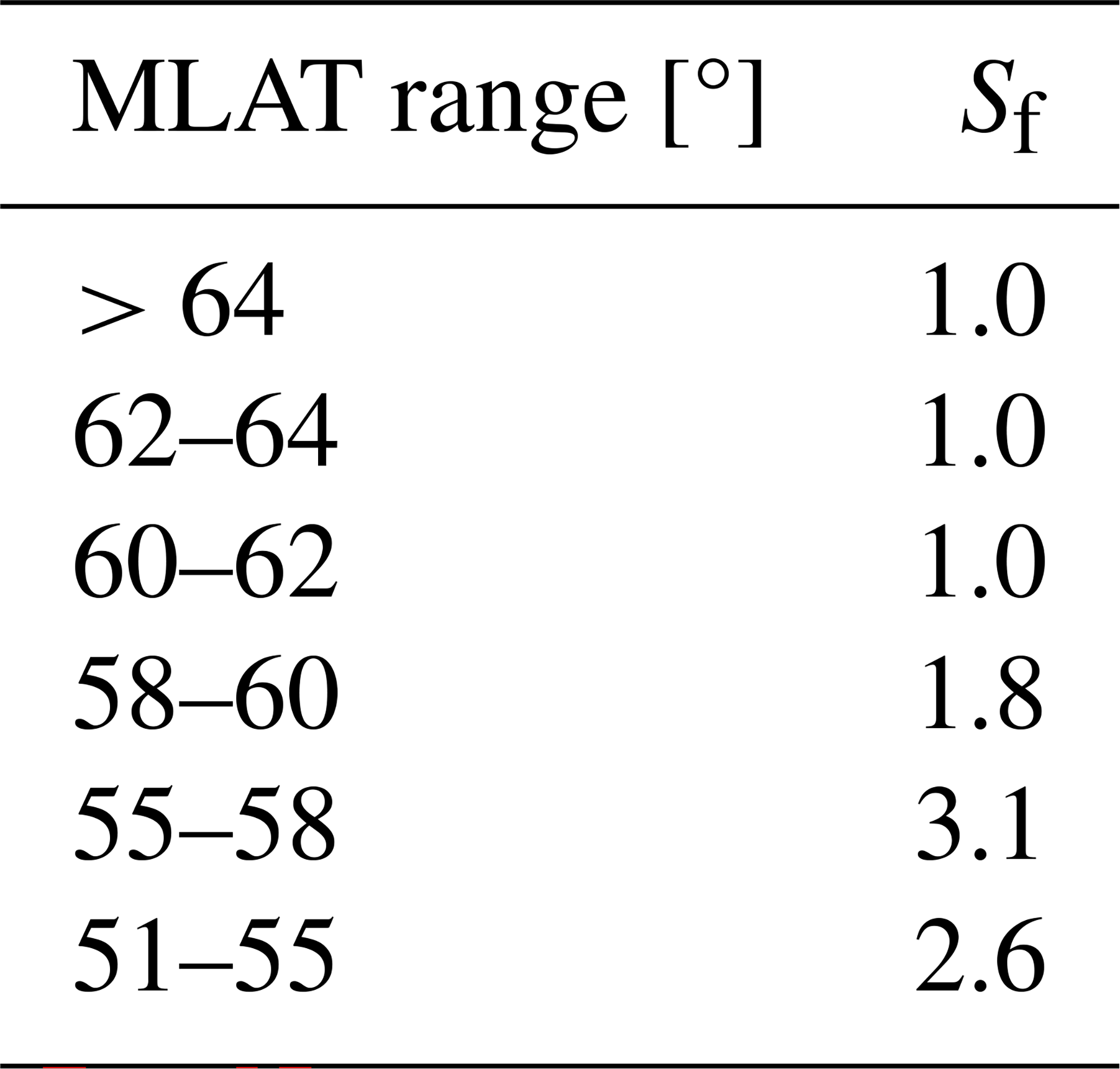
The fourth step involves scaling the E_H to represent a worst-case scenario. To achieve this, a scaling factor (S_f) is applied to generate a physically plausible 1-in-100-year event. By “plausible”, we refer to a geoelectric field whose magnitude peaks near the characteristic geomagnetic latitude threshold where extreme driving is expected. This threshold is generally expected to lie between 53 and 62° geomagnetic latitude, as suggested by Thomson et al. (2011). Then, we scaled the geoelectric field values by adopting the results from Lanabere et al. (2024), who estimated the 1-in-100-year return levels of the 1D geoelectric field at various locations in Sweden. Although these estimates are based on a 1D Earth conductivity model, the authors also provide normalized scaling factors relative to the peak geoelectric field observed during the 2003 Halloween storm. In their results, the three northernmost sites exhibit return levels slightly below the October 2003 E_H field peak, yet still within the 95 percent confidence interval. As a result, for these high-latitude locations, we adopt a conservative scaling factor of S_f=1. The scaling factor varies with magnetic latitude, and the values in different magnetic latitude ranges are indicated in Table 2. We mention that we do not take into account the secular variation of the magnetic field, which is expected to show a great impact in Sweden since the change of the magnetic field during the last 40 years resulted in a shift toward lower latitudes.

Table 2 Scaling factors (S_f) applied to the horizontal geoelectric field (E_H) from the 30 October 2003 Halloween event to construct a physically plausible 1-in-100-year scenario across different geomagnetic latitude bands. Values based on the results of Lanabere et al. (2024).

Finally, in step five, the scaled E_H was used as input to the RAISE model (Rosenqvist et al., 2025) to compute the voltage time series for each of the 335 power grid lines. We report only the power line voltages, which represent the E_H integrated along the line's path, as the true line resistances required to estimate currents are considered sensitive information and a matter of national security. Assuming resistances to estimate currents would introduce additional uncertainty. Nevertheless, the total voltages provide a valuable and meaningful metric for assessing the impact on the grid and can serve as a proxy for GICs, as they can later be converted to currents by the power grid operator.

3.1 Case 1: Halloween geomagnetic storm

The magnetic field time series used in Case 1 are presented in Fig. 1 and visualized in more detail in the animation Case1_BE.mp4 (panels a, b, c), which consists of frames spanning 19:40 to 20:30 UT (50 min) with a 10 s timestep. Figure 1a shows the interpolated horizontal magnetic field component (B_H), based on data from the magnetic stations marked with black dots. The magnetic field components B_x and B_y time series at the locations indicated by a star in Fig. 1a are presented in Fig. 1b, c. Around 19:47 UT, a local substorm onset occurred, marked by the initial drop in B_x, indicating the presence of a WEJ centred over the Fennoscandian region. During this period the WEJ peaked ∼ 19:53:00–19:58:00 and ∼ 20:02:00–20:08:40 UT, which have been suggested to be caused by dipolarization of the nightside inner magnetosphere (Juusola et al., 2023). This is also observed in the B_H time series at the locations indicated by a star in Fig. 1a, each location representing a different MLAT band in Sweden. B_x peaks around 19:56 in Northern Scandinavia (>60° MLAT), a few minutes later B_x peaks in central and Southern Scandinavia (54–60° MLAT) around 20:04. Finally, a secondary B_x depression appeared at latitudes above 60° MLAT, followed by an abrupt weakening of B_x and a concurrent increase in B_y between 20:08 and 20:10 UT.

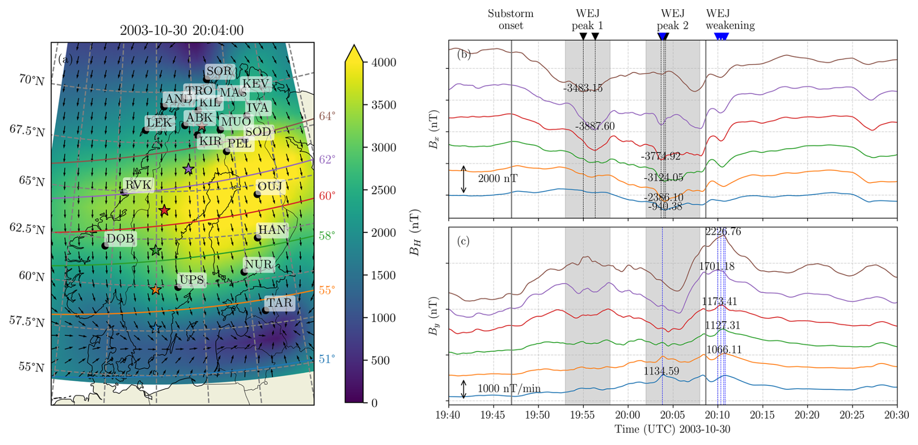
Figure 1 Ground magnetic field estimation during the 30 October 2003 geomagnetic storm. (a) Interpolated magnitude (shaded) and direction (arrows) of the horizontal magnetic field (B_H) at 20:04 UT, the time when most stations recorded their maximum B_H. (b) Interpolated time series of the north-south B component (B_x), and (c) east-west B component (B_y) at the locations indicated by a star in panel (a). The vertical black dashed lines indicate the B_x peaks, and the blue dashed lines indicate the peaks in B_y. The coloured stars in panel (a) mark the sites where time series data were extracted.

The maximum estimated E_H between 19:40 and 20:30 UT is summarized in Fig. 2a, together with the E_H time series at the locations marked by stars in Fig. 2b, c. The maximum values of the horizontal geoelectric field (Max(E_H)) occur along the Norwegian coast due to the well-known coastal effect (Gilbert, 2005) with values of 10 up to ∼30 V km⁻¹. During this time interval, regions of Sweden distant from the north-west coast experienced E_H values around 2 V km⁻¹, with local maxima between 4 and 8 V km⁻¹ in areas with pronounced conductivity gradients, and generally remaining below 1 V km⁻¹ in regions of high conductivity.

The time series in Fig. 2b, c shows that almost all locations experienced the maximum $\mathrm{d}{B}_{\mathrm{H}}/\mathrm{d}t=\sqrt{{\left(\mathrm{d}{B}_x/\mathrm{d}t\right)}^{\mathrm{2}}+{\left(\mathrm{d}{B}_y/\mathrm{d}t\right)}^{\mathrm{2}}}$ at the moment of the abrupt weakening of the WEJ at 20:08:30 UT, with a maximum near 62° MLAT (violet line). The magnitude gradually decreases at higher latitudes and drops off more sharply toward lower latitudes. The peaks in E_H generally occur during periods of elevated $\mathrm{d}{B}_{\mathrm{H}}/\mathrm{d}t$. However, the maximum values of E_H do not coincide exactly with the peaks in $\mathrm{d}{B}_{\mathrm{H}}/\mathrm{d}t$. We notice that the time series around 60° MLAT (red line) presents relatively larger E_H values during the whole substorm.

The E_H maps during the evolution of the substorm are provided in the animation Case1_BE.mp4 (panel e). In Sweden, large E_H values first appear in the north at the times when the WEJ peaks (19:55 UT), then shifts toward central Sweden by 19:58 UT, and reach lower latitudes near 20:04 UT (second WEJ peak), affecting a broad area of southern and central Sweden. Four minutes later, at 20:07:20 UT, the E_H maximum moves back to higher latitudes as the substorm evolves. Large geoelectric fields are again observed in central and southern Sweden around 20:08:50 UT, just after the WEJ weakening.

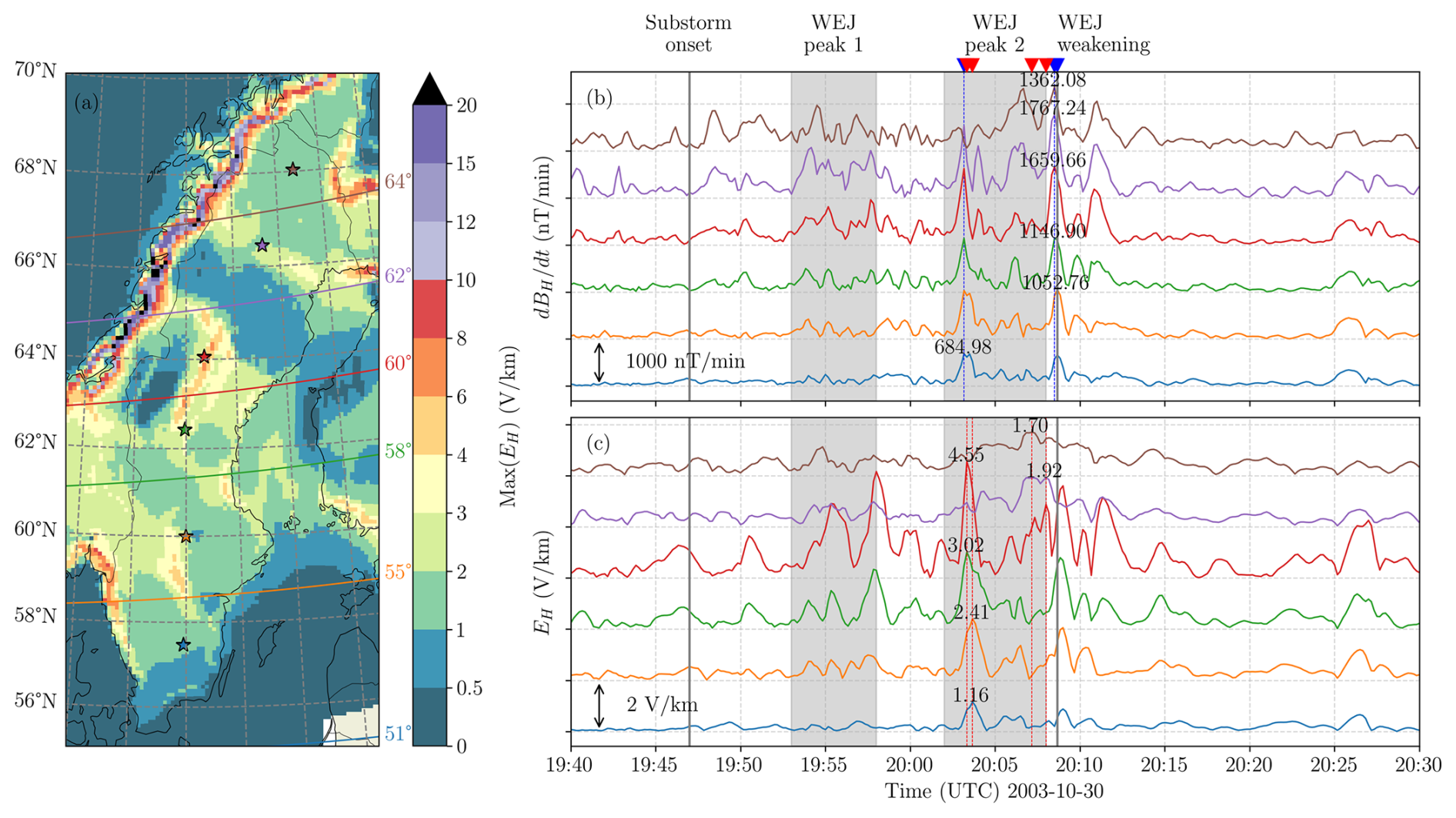
Figure 2 Case 1: Map of the maximum geoelectric field magnitude during the interval 19:40–20:30 UT. The colour scale indicates the peak geoelectric field strength at each location. Coloured stars mark the same sites as in Fig. 1a, where the temporal $\mathrm{d}{B}_{\mathrm{H}}/\mathrm{d}t$ and E_H profiles were extracted and shown in the panels (b) and (c) respectively. The vertical dashed lines indicate the moment of the series peak.

The E_H values were scaled to a 1-in-100-year event according to the MLAT bands presented in Table 2. The scaled E_H and the corresponding response in the Swedish power grid are illustrated in more detail in the animation Case1_EGrid.mp4. In northern Sweden, where the scale factor is 1 (i.e., no scaling is applied), maximum E_H values reach only about 2 V km⁻¹. In contrast, southern and central Sweden show E_H about 2–6 and 6–10 V km⁻¹ respectively. The largest E_H values are observed between 55 and 58° MLAT, with values of around 6–10 V km⁻¹ and a peak of approximately 12–15 V km⁻¹ occurring in regions with pronounced conductivity gradients (Midskog, Töreboda, Söderhamn, Vittersjö, Göteborg). The maximum scaled E_H is summarized in Fig. 6 and will be described in Sect. 4.

3.2 Case 2: Simplified Uniform External Magnetic Field

In Case 2, we assume that a large-scale ionospheric current covers all Fennoscandia. The ionospheric equivalent current shown in Fig. 3a confirms that a current system was indeed present, but was limited to northern and central Fennoscandia, with a maximum between Finland and Sweden. The right panel of Fig. 3 shows B_H,ext and its time derivative at the magnetic stations along Finland and Estonia (solid lines) and in Sweden (dashed lines). This highlights the waveform variations across latitudes, showing similarities among the higher-latitude and, separately, among the lower-latitude, though with notable differences in amplitude. The maximum $\mathrm{d}{B}_{\mathrm{H},\mathrm{ext}}/\mathrm{d}t$ is observed almost simultaneously across all locations at 20:08:30 UT, with a maximum near 60° MLAT (red line). The $\mathrm{d}{B}_{\mathrm{H},\mathrm{ext}}/\mathrm{d}t$ magnitude gradually decreases at higher latitudes and drops off more sharply toward lower latitudes. Due to the latitudinal differences in the waveforms, we had to determine which one was most representative of the current system to later apply it across the entire region. As a first approach, we selected the waveform from the OUJ station, as it was located near the centre of the ionospheric current and exhibited the largest $\mathrm{d}{B}_{\mathrm{H},\mathrm{ext}}/\mathrm{d}t$. We also considered the magnetic field data from the HAN station, which showed a similar evolution but with a lower $\mathrm{d}{B}_{\mathrm{H},\mathrm{ext}}/\mathrm{d}t$. Data from these two stations were used to compute the ground geoelectric field, and the waveform that produced the largest geoelectric field was selected.

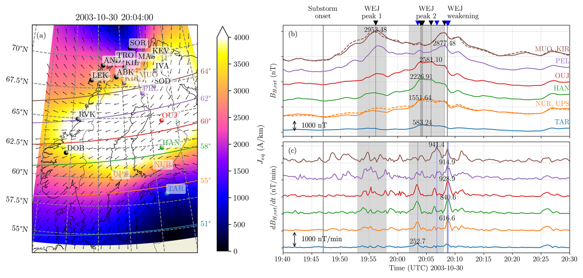
Figure 3 Ground-based estimations during the 30 October 2003 geomagnetic storm. (a) Ionospheric equivalent current (J_eq) magnitude (shaded) and direction (arrows) at 20:04 UT, the time when most stations recorded their maximum B_H and the J_eq reaches its minimum latitude. (b) Time series of the external part of the horizontal magnetic field magnitude (B_H,ext), and (c) Magnetic field perturbations ($\mathrm{d}{B}_{\mathrm{H},\mathrm{ext}}/\mathrm{d}t$) at the magnetic stations along Finland and Estonia (solid line) and in Sweden (dashed line). The vertical black dashed lines indicate the B_H peaks, and the blue dashed lines indicate the peaks in $\mathrm{d}{B}_{\mathrm{H},\mathrm{ext}}/\mathrm{d}t$.

The 3D geoelectric field response in Sweden, computed using uniform magnetic field waveforms from OUJ and HAN ground-based stations as inputs, is shown in Fig. 4. Differences in induced E_H at fixed positions are primarily driven by variations in the input B_H,ext. Although the OUJ and HAN stations exhibit similar B_H,ext waveforms (Fig. 4a, d), the magnitude and perturbations are larger at OUJ; however, the induced geoelectric fields calculated using B_H,ext from HAN at the locations marked with stars in Fig. 1a were greater than those calculated using B_H,ext from OUJ. This highlights how the geoelectric field is strongly influenced not only by the local ground conductivity but also by the frequency content of geomagnetic field variations. As shown in Dimmock et al. (2024, Fig. 9), two distinct $\mathrm{d}H/\mathrm{d}t$ peaks are observed around the time of the transformer trip event, yet the largest peak in the geoelectric field corresponds to the smaller of the two $\mathrm{d}{B}_{\mathrm{H}}/\mathrm{d}t$ peaks, further illustrating the non-linear and frequency-dependent nature of the relationship between magnetic and geoelectric fields.

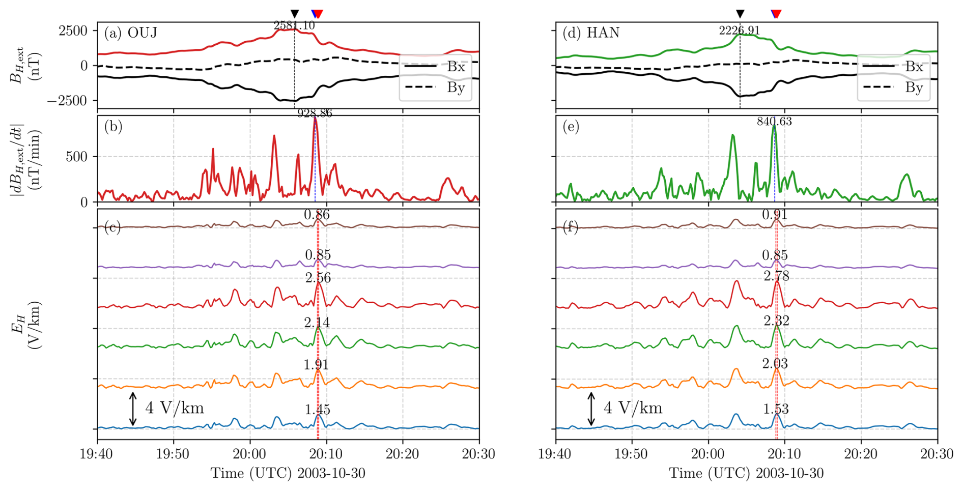
Figure 4 Case 2: Estimated 3D horizontal geoelectric field during 30 October geomagnetic storm using two different magnetic field waveform inputs. (a, d) Magnitude of the external component of the horizontal magnetic field (B_H,ext) from the OUJ and HAN stations, respectively. (b, e) magnetic field perturbations. (c, f) horizontal geoelectric field time series at the fixed locations shown with stars in Fig. 1a.

For the scenario evaluated in this study, we chose the HAN station waveform, which resulted in the largest E_H response. However, we note that this is not a unique, but rather a representative selection for worst-case assessment. In the case of a spatially uniform magnetic field, the geoelectric field differences across the country purely depend on the ground conductivity. The time evolution of B_H,ext, $\mathrm{d}{B}_{\mathrm{H},\mathrm{ext}}/\mathrm{d}t$ and E_H is shown in the animation Case2_BE.mp4. The maximum E_H is detected around 20:09 UT, just after the $\mathrm{d}{B}_{H,\mathrm{ext}}/\mathrm{d}t$ peak, however the magnitude is smaller than Case 1 since we are evaluating the E_H from the external part of B_H. A second relative E_H maximum is detected at 20:03:40 UT. As in Case 1, we scaled the E_H field values to be a 1-in-100-year event using the scaling factors in Table 2. The animation for the scaled E_H using HAN station waveform as input and the power line voltages are shown in Case2_EGrid.mp4.

3.3 Comparison of Scaled E_H between Case 1 and Case 2

A snapshot at the time of the scaled E_H peak (20:03:40 UT) for Case 1 and Case 2 are shown in Fig. 5a, b, and the difference between both cases in Fig. 5c. Above 62° MLAT, the largest differences are confined to the Norwegian coast, likely due to variations in the B waveform at high latitudes between the two cases. In Fig. 5a, b, Case 1 shows southward-oriented E on the seaside and landside of the Norwegian coast, while Case 2 exhibits eastward-oriented E at both sides. Between 58 and 62° MLAT, the differences are minimal because the magnetic field input in Case 1 at these latitudes is mainly dominated by the observations in HAN and OUJ, which are very similar to the input used in Case 2. The remaining variations can be mainly attributed to the difference between B_tot and B_ext.

Below 60° MLAT, the differences become more evident. In the 55–58° MLAT band, both cases present the largest maximum scaled E_H, but for Case 1 E_H is larger than in Case 2, particularly in the western region due to pronounced conductivity gradients, as well as along the east coast. In southern Sweden (51–55° MLAT band), the scaled E_H values in Case 2 exceed those in Case 1 by about 4 V km⁻¹ at the coasts. This difference is mainly related to the larger B magnitude and perturbations obtained in Case 2 compared to those derived from the B interpolation, which is strongly affected by the lack of magnetic field measurements in southern Sweden and relies primarily on interpolation from the TAR magnetic station.

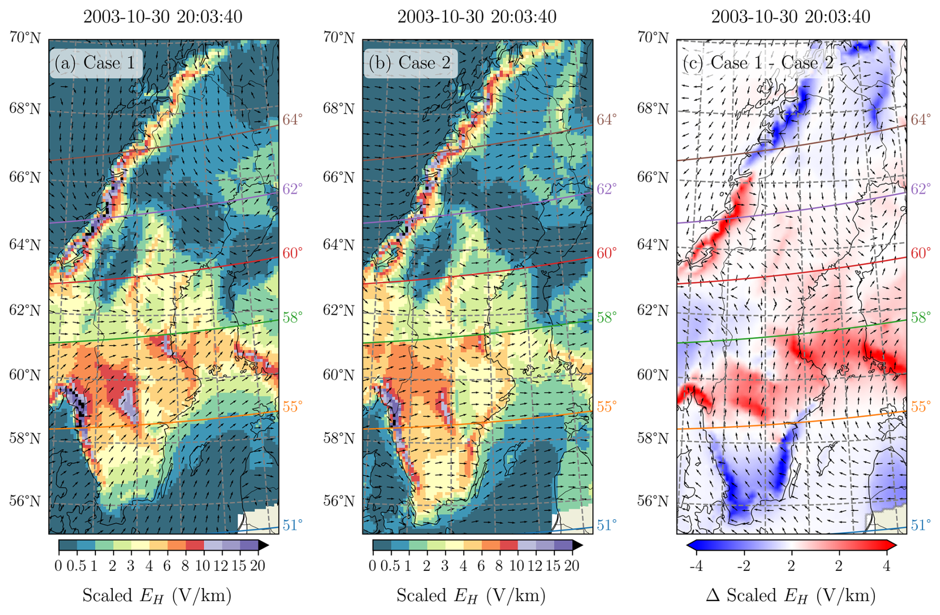
Figure 5 Comparison between the scaled E_H for Case 1 and Case 2. Panels (a) and (b) show the E_H magnitude (shaded) and direction (arrows) at 20:03:40 UT for Case 1 and Case 2, respectively. Panel (c) Shows the difference in scaled E_H between Case 1 and Case2. Blue (red) shaded colour indicate that the scaled E_H magnitude in Case 1 in larger(lower) than in Case 2 (shaded) and arrows are the difference in the scaled E_H direction.

4 Swedish power grid impacts

The impact on the Swedish power grid is limited to the analysis of the induced voltages in the transmission lines, calculated by integrating the geoelectric field along the power lines under the two 1-in-100-year scenarios. To complement the total induced voltage, we also compute the voltage per kilometre, which corresponds to the line-averaged geoelectric field projected along the transmission line direction. This provides a measure of the effective geoelectric driving experienced by each line, independent of its length. We acknowledge that this does not represent the full behaviour of the Swedish power grid as a connected network. However, large induced voltages (Voltages > 100 V) have been related to several issues during the March 1989 geomagnetic storm (Lucas et al., 2018).

A proper GIC assessment would require detailed and time-accurate information on grid topology, transformer resistances, grounding configurations, and relay-protection settings. These engineering parameters are not publicly available at the level of detail required for reliable modelling the power grid. For this reason, it is not currently feasible to determine what would constitute a true worst-case scenario for the power grid itself, nor to model specific impacts such as transformer saturation or protection-system behaviour. Our study therefore focuses deliberately on the geoelectric field forcing, consistent with how Svenska kraftnät defines major events (based on the physical NOAA G-scale rather than grid-hardware responses). Moreover, large global geomagnetic disturbances, typically associated with locally enhanced geoelectric fields, are known to increase the likelihood of power-grid disturbances (Rosenqvist et al., 2025).

The impact on the Swedish power grid for the Case 1 worst-case scenario is summarized in Fig. 6. The maximum scaled E_H between 19:40 and 20:30 UT reaches approximately 8 V km⁻¹ in at least four regions: the southwest coast near Göteborg, the central east coast near Vittersjö, central Sweden near Midskog, and central Sweden near Karlstad. Around these areas, the maximum power line voltage per km exceeded 3.34 V km⁻¹ (red lines in Fig. 6b), which corresponds to the 80th percentile of the maximum voltage per km across all lines. Power lines that exceeded 3.34 V km⁻¹ are typically short east–west oriented, but some north–south oriented lines near regions of high E_H are also present (e.g., Vittersjö, and south-west Sweden). In contrast, power lines with voltages per km below the 20th-percentile maximum voltage per km (1.17 V km⁻¹) throughout the storm (black lines) are mainly located in northern Sweden and at the far south, but notably, some are also found near the Stockholm area close to lines showing high voltages, highlighting the complexity of the system.

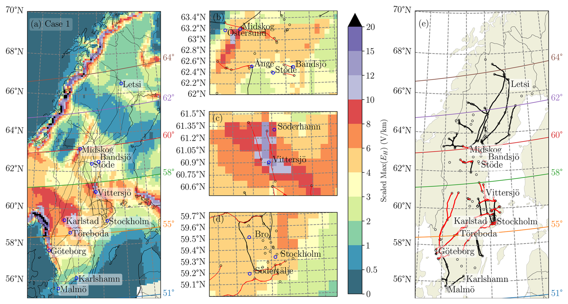
Figure 6 Case 1: (a) Maximum scaled E_H across Sweden during the period 19:40:00–20:30:00 UT on 30 October 2003. Panels (b), (c), and (d) show zoomed-in views for the Midskog, Vittersjö, and Stockholm regions, respectively. (e) Power lines exceeding the 80th percentile of the maximum voltage per km during the whole period (3.34 V km⁻¹, in red), and power lines that remained below the 20th percentile (1.17 V km⁻¹, in black).

For Case 2, the maximum scaled E_H and resulting power line impacts differ from Case 1, particularly in southern Sweden, due to the larger E_H values in this region as previously discussed in Fig. 5 and also evident from Fig. 7a. Consequently, power lines exceeding the 80th percentile of the maximum voltage per km across all lines for Case 2 (2.76 V km⁻¹) appear even at lower latitudes in Fig. 7e.

In both cases, the lines that did not exceed the 20th percentile maximum voltage per km (0.75 V km⁻¹) are primarily north–south oriented in central and southern Sweden, while in northern Sweden, lines of any orientation generally did not experience high voltages per km.

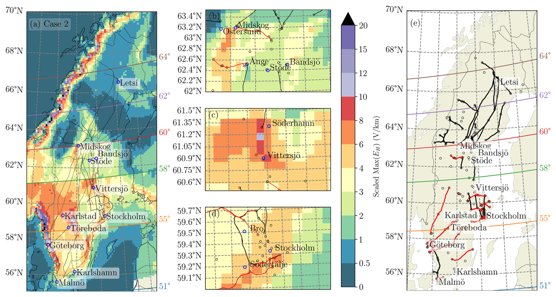
Figure 7 Same as Fig. 6, but for Case 2. (a) Maximum scaled E_H across Sweden during the period 19:40:00–20:30:00 UT on 30 October 2003 and zoom-in views (b–d) around Midskog, Vittesjö and Stockholm. (e) Power lines exceeding the 80th percentile of the maximum voltage per km during the whole period (2.76 V km⁻¹, in red), and power lines that remained below the 20th percentile (0.75 V km⁻¹, in black).

Östersund, Midskog, Bandsjö, Stöde, Ånge, Söderhamn, Vittersjö, Karlstad, Töreboda, and the Stockholm area have been previously identified as vulnerable to GIC impacts (Kappenman, 2006; Hapgood, 2019; Dimmock et al., 2024; Rosenqvist et al., 2025). Figures 6a and 7a show that these locations lie in close proximity to regions of elevated E_H in both worst-case scenarios. Their large E_H values appears to be linked to nearby zones of pronounced lateral conductivity gradients, which emerge as a critical risk factor. Interestingly, Malmö, which experienced a GIC-induced blackout in 2003, does not appear as a major hotspot in the Case 1 results. This may be attributed to the limited magnetometer coverage in southern Sweden (MLAT < 55°) during the Halloween event, as well as uncertainties in the regional conductivity model. Notably, Malmö is identified as vulnerable under Case 2, when a large-scale ionospheric current system is assumed.

A particularly noteworthy case is Karlshamn, which appears susceptible to GICs even under relatively low E_H values, between 0.42 and 0.75 V km⁻¹, according to Table 1 in Rosenqvist et al. (2025). As with Malmö, this behaviour may be influenced by sparse magnetometer coverage in southern Sweden and by limitations in the conductivity model. In addition, the most intense GICs are often observed at substations located near the edges of a power-grid network (Viljanen et al., 2012). Both Malmö and Karlshamn lie along the southern boundary of the Swedish transmission system, which may enhance their vulnerability. These examples highlights how local grid topology and substation characteristics may influence vulnerability independently of regional E_H strength.

4.1 Comparison between Case 1 and Case 2

For each line, we computed its orientation by assuming a straight line between its starting and ending geographic positions. This analysis shows that the network is largely north–south oriented, with 63 % of the lines having angles greater than 45°, reflecting the country’s elongated shape. East–west oriented lines (angles less than 45°) are mainly concentrated within the latitude band 58–64° N, which is also where most lines are located, as shown in Fig. 6a.

The maximum voltage for each line during the two worst-case scenarios, categorized by its orientation, is summarized in Fig. 8. Voltages are highest for north–south oriented lines, which are typically the longest. However, when normalized by line length, east–west oriented lines exhibit the largest values, ranging between 6–8 V km⁻¹ due to the dominant east-west orientation of the E_H (specially for Case 2). In general, the voltage in the line increases with length as shown in Fig. 8c; however, because line resistance also increases with length, longer lines might not contribute significantly higher induced currents. Lines shorter than 20 km did not reach the level of 100 V in either scenario, and voltages above 10 V begin to appear for lines longer than 2 km. The median length of the 335 transmission lines is 53 km. For lines longer than 50 km, 73 % experience voltages above 100 V at least once in Case 1, and 60 % in Case 2. These fractions decrease to 37 % and 28 %, respectively, when the threshold is raised to 200 V, which still represents a substantial number of affected lines.

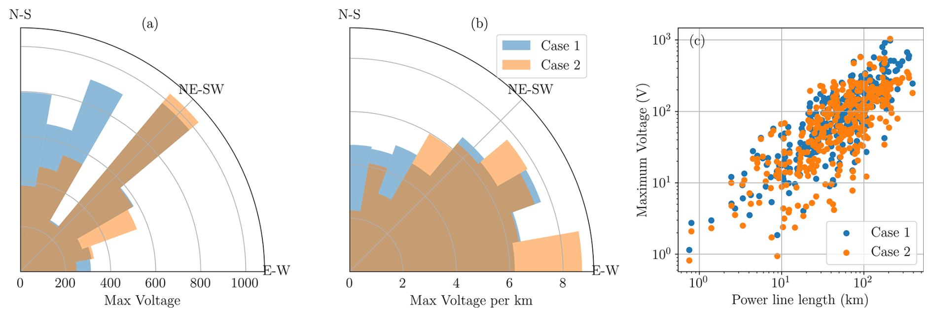
Figure 8 (a–b) Maximum voltage and voltage per km (V km⁻¹) by power line orientation. (c) Relation between the power line length and the maximum voltage reached for the Case 1 and Case 2 worst-case scenarios.

Finally, for both worst-case scenarios, the number of power lines experiencing voltages exceeding 10 V easily exceeds 100 lines on more than 9 occasions during the analyzed period, while about 100 lines exceed 50 V at different stages of the substorm, as illustrated in Fig. 9. Among these 100 lines, 16, 7, and 1 lines are connected near the main Swedish cities of Stockholm, Göteborg, and Malmö, respectively. At the moment of the WEJ weakening around 100 lines experienced voltages larger than 100 V. Of these, 6 lines were located near Stockholm and 7 near Göteborg, while no lines around Malmö exceeded the 100 V threshold.

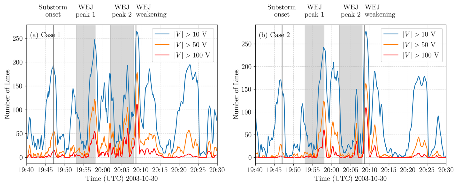
Figure 9 Number of lines exceeding Voltages $\left|V\right|>\mathrm{10}$ V (blue), $\left|V\right|>\mathrm{50}$ V (orange), and $\left|V\right|>\mathrm{100}$ V (red) for the worst-case scenarios (a) Case 1 and (b) Case 2.

5 Discussion

This study presents the first assessment of a worst-case scenario for the entire Swedish power grid using real data during the development of a premidnight substorm event. We applied the recently developed RAISE model (Rosenqvist et al., 2025) to evaluate the impacts of an extreme horizontal geoelectric field, representative of a 1-in-100-year event, on the Swedish power grid. To represent this extreme event, we derived the induced E_H from the 30 October 2003 Halloween geomagnetic storm between 19:40 to 20:30 UT and subsequently scaled it to a 1-in-100-year level using return periods reported in (Lanabere et al., 2024). We conducted the analysis following two different approaches, reflecting the fact that there is no exact definition of what constitutes an extreme event. From the perspective of scaling existing measurements, we identified two plausible options and aimed to explore both. This allowed us not only to evaluate the impacts under each assumption but also to assess the sensitivity of the results to the choice of approach. In Case 1, we used actual magnetic field observations across Fennoscandia to estimate the E_H in Sweden. This case accounts for the combined effect of regional magnetic field waveforms and spatial variations in ground conductivity. In Case 2, we assumed the presence of a large-scale ionospheric current system located over Fennoscandia, resulting in the same temporal pattern of magnetic field perturbations across Sweden. Consequently, the variability in the E_H arises solely from differences in ground conductivity.

5.1 Maximum estimated and observed E values

In this study, the induced E_H for the Halloween event was scaled to represent a 1-in-100-year scenario. In particular, a scaling factor of three was used within the 55–58° MLAT band, representing a conservative lower bound. Based on the 95th percentile confidence interval of (Lanabere et al., 2024), the scaling could be as high as a factor of five. This implies our modeled scenario likely underestimates the potential severity, providing a lower limit benchmark for extreme conditions. Nonetheless, even under this conservative scaling, maximum E_H values reached approximately 10–12 V km⁻¹ between 55 and 58° MLAT.

These values are consistent with estimates for the May 1921 storm, which exceeded the 1-in-100-year return level and caused catastrophic damage to the telegraph and telephone station at Karlstad, where geoelectric fields likely reached ∼10 V km⁻¹, as discussed by Hapgood (2019) and references therein. Hapgood (2019) also reports other impacts in Sweden: Östersund and Söderhamn experienced very large earth currents; Telephone lines between Göteborg and Stockholm were unstable and GIC measurements of about 1.1 A; a minor fire at the telegraph and phone station of Ånge. The suggested E_H=10 V km⁻¹ in Karlstad discussed in Hapgood (2019) is close to the range of 10–12 V km⁻¹ of the scaled E_H of both worst-case scenarios.

In the case of the 13–14 July 1982 storm, which was weaker than the Halloween event (Dst minimum of −325 nT), the voltage peak value in telecommunication cables between Södertälje-Stockholm and Bro-Stockholm was roughly 80 V, implying an estimated east–west-oriented geoelectric fields of approximately 4–5 V km⁻¹ (Wik et al., 2009). In Figs. 6e and 7e, a power line in Södertälje appears in the lines exceeding Voltages per km >3 V km⁻¹. However, during the 1982 event, highly localized geoelectric fields of up to 9.1 V km⁻¹ were inferred from observations along a short 921 m segment of the 100 km railway communication line between Stockholm and Töreboda (Kappenman, 2006). Notably, Töreboda lies within the 55–58° MLAT band, crosses a region with pronounced conductivity gradients, and the E_H values in both cases exceeds 10 V km⁻¹.

In the reference study by Pulkkinen et al. (2012), maximum E_H values of 20 V km⁻¹ were assumed for resistive ground structures above the MLAT threshold (i.e., the magnetic latitude where maximum geomagnetic disturbances and geoelectric fields typically occur) and 5 V km⁻¹ below it, while for conductive ground structures the corresponding values were 2 and 0.5 V km⁻¹. In our analysis, we find scaled E_H values exceeding 20 V km⁻¹ in highly localized regions near the west coast. However, the choice of 2 V km⁻¹ for conductive ground areas above the MLAT threshold in Pulkkinen et al. (2012) appears somewhat higher than our estimates, which range between 0.5 and 1 V km⁻¹. Below the MLAT threshold, their maximum values for resistive ground (5 V km⁻¹) are consistent with our results, where we obtain maximums of 4 to 6 V km⁻¹. For the 0.5 V km⁻¹ limit in conductive areas below the MLAT threshold, no direct comparison with our analysis is possible.

5.2 Power grid implications

To prevent permanent transformer damage from GICs, the Swedish power grid requires that new transformers withstand a direct current of 200 A for 10 min while operating at full load (private communication with Johan Setréus, Svenska Kraftnät). Since the actual line resistances are considered sensitive information, we adopted a constant ground resistance of R_GR=0.5 Ω and line resistances of $r_{\mathrm{L},\mathrm{220}}=\mathrm{0.022}$ Ω km⁻¹ and $r_{\mathrm{L},\mathrm{400}}=\mathrm{0.008}$ Ω km⁻¹, following the values used by Viljanen et al. (2012). Based on these assumptions, we find that GICs of 200 A can be reached even in short (<20 km) 220 and 400 kV lines under a E∼10 V km⁻¹ oriented parallel to the line. However, such large E values, and consequently large currents, typically occur only in very short bursts rather than being sustained. The 10 min requirement is also ambiguous: it is unclear whether it refers to continuous or cumulative current exposure. Moreover, this specification applies only to the newest transformers, and no information is available for the tolerances of different units. These results are important since they show that the 200 A limit can be reached, however a future study will be required to determine the impact on Swedish transformers.

We have shown that during intervals of very active ionospheric current variations, particularly during substorm activity, large $\mathrm{d}B/\mathrm{d}t$ and E_H values were estimated at latitudes below 60° MLAT. As a consequence, several power lines exceeded high voltage thresholds (e.g., approximately 100 power lines experienced induced voltages exceeding 50 V at several times during the substorm period). For comparison, Lucas et al. (2018) reported that 62 transmission lines exceeded 100 V during the March 1989 geomagnetic storm, which triggered a major blackout in the Hydro-Québec power system. Although power-grid disturbances do not always coincide with the time of peak voltage or geoelectric field (Dimmock et al., 2024; Wallner et al., 2026), or with peak GICs (Pulkkinen et al., 2005), intervals of high induced voltages still imply larger voltage variations.

The large number of power lines subjected to high induced voltages in our scenario could lead to elevated GICs, which in turn may affect protection relays. Relay misoperations are often linked to harmonics, inappropriate relay types or settings, or faulty relay systems, rather than to the voltage magnitude itself. Collapse can be initiated by one or several coincident relay misoperations, each removing a transformer or line from service while its integrity is verified. Based on this, relay actions may occur during intervals of high or rapidly changing rates of change voltage rather than strictly at maximum voltage.

Understanding which combinations of geoelectric field, induced voltage, network configuration, and system state lead to real incidents remains an open problem and requires further investigation. Such studies will soon be possible with the recently installed GIC monitoring device in Karlshamn, connected to the transformer neutral-to-earth point and deployed by the Swedish transmission system operator, Svenska Kraftnät.

5.3 Future implications

This study builds on a series of investigations in Sweden that have significantly advanced understanding of induced geoelectric fields and the power grid’s response to geomagnetic activity (e.g., Wik et al., 2008, 2009; Wintoft et al., 2016; Dimmock et al., 2019; Rosenqvist and Hall, 2019; Rosenqvist et al., 2022; Lanabere et al., 2023, 2024; Dimmock et al., 2024; Rosenqvist et al., 2025; Wallner et al., 2026). Expanding on this foundation, we provide the first detailed and comprehensive assessment of the potential impacts of a 1-in-100-year ground geoelectric field on the Swedish power grid. Importantly, our analysis is based on total voltage, representing the geoelectric field integrated along each line’s path. Because information on individual line resistances is not available, we could not convert voltages into GICs. Future versions of the RAISE model may incorporate this capability.

The main goal of this study is to benchmark an extreme geoelectric field event and understand how it could affect the power grid, given the known layout. This has provided meaningful insights into regions that may be at risk. We also assessed the number of lines that could be subjected to hazardous GICs during a 1–100 year event. An added benefit of this work is that Svenska Kraftnät can use this knowledge for their own investigations using realistic grid configurations. We view this work as a significant advancement for Sweden in understanding the effects of rare, high-impact events.

A particularly important finding concerns the behaviour of substations in southern Sweden. Substations such as Malmö and Karlshamn, show weaker E_H responses than expected despite their documented vulnerability to GICs. This behaviour is likely influenced by the limited magnetometer coverage in southern Sweden (MLAT < 55°) and by uncertainties in the regional conductivity model, both of which may lead to underestimated impacts in this region. In addition, both substations lie along the southern edge of the Swedish transmission grid, where GICs are often amplified due to network topology effects. Together, these factors highlight the need for extending the magnetometer array into southern Sweden, updating the regional conductivity model, and improving the representation of the power grid topology in this area.

Moreover, there are still many unanswered questions to address, such as the following: (1) How do small-scale ionospheric currents (<1000 km) during major geomagnetic storms influence the spatial variability of geoelectric fields and GICs? (2) Is the current number of magnetometers sufficient to adequately capture space weather impacts in low MLAT regions, particularly in areas of large conductivity gradients? (3) Are power grid operators equipped and prepared to manage simultaneously high induced voltages occurring on multiple power lines during extreme geomagnetic storms? (4) What defines an extreme event from the perspective of the electricity-system owner and operator? Our aim is to continue to address these key questions in future studies.

6 Conclusions

We used the recently developed RAISE model (Rosenqvist et al., 2025) to investigate the impacts in the Swedish power grid during a 1-in-100 year geoelectric field event. The main findings from this study are summarized as follows:

1. The largest scaled E_H are found in localized areas with pronounced lateral conductivity gradients, reaching up to ∼ 12 V km⁻¹, and in the western part of the 55–58° MLAT band where conductance is particularly low.

2. North-South-oriented power lines experience larger total induced voltages because their overall length is greater than that of East-West lines. However, East-West lines show larger voltages per kilometer, mainly because they are located south of 60° MLAT, where the largest geoelectric fields are calculated.

3. Voltage per km larger than the 80th percentile of maximum voltage per km across all lines (3.34 V km⁻¹ for Case 1 and 2.76 V km⁻¹ for Case 2) are concentrated near substations that have historically reported GIC disturbances, including Midskog, Bandsjö, Vittersjö, and the Stockholm area.

4. In western Sweden, several power lines exhibit voltage per km larger than 3.34 V km⁻¹ for Case 1 and 2.76 V km⁻¹ for Case 2 even when oriented northwest–southeast, primarily due to localized conductivity structures. In eastern Sweden, for Case 1, the power lines exceeding the 80th percentile of maximum voltage between Vittersjö and Söderhamn are oriented north-south along an area of very large E_H values.

5. Interestingly, the Karlshamn substation, identified in previous studies as GIC-prone, does not exhibit high E_H levels, even when assuming a uniform ionospheric current system.

6. The weak responses observed in Malmö in Case 1, despite its documented blackout in 2003, is likely due to limited magnetometer coverage in southern Sweden (MLAT < 55°) and to inaccuracies in the regional conductivity model, which may lead to underestimated impacts in this region under real conditions.

7. During the WEJ peaks and sudden weakening in the worst-case scenarios, around 100 power lines exceeded 50 V multiple times during the substorm. At the moment of the WEJ weakening, close to the time of maximum $\mathrm{d}{B}_{\mathrm{H}}/\mathrm{d}t$, about 100 lines exceeded 100 V.