Mapping transition region flows to the ionosphere in a global hybrid-Vlasov simulation

The dynamics of the inner magnetosphere and magnetotail are determined by a number of factors such as magnetic reconnection, plasma instabilities, and large-scale plasma motion. We use the global hybrid-Vlasov simulation Vlasiator to study these dynamics as well as their signatures in the ionosphere. We observe magnetic reconnection, fast flows, and vorticity in the transition region between the Earth's dipolar field and the magnetotail. In our simulation, reconnection is first triggered at the dawn and dusk sides of the magnetotail current sheet. It then spreads across the current sheet. Concurrently, an azimuthally periodic, wave-like density structure develops in the transition region along with fast Earthward flows and enhanced vorticity patterns. The Earthward flows and vorticity induce field-aligned currents, which map onto the ionospheric simulation domain, creating a patchy current distribution. We find that the event is driven by the combination of reconnection-induced fast flows and the ballooning/interchange instability.

1 Introduction

The transition region between the Earth's dipolar magnetic field and the magnetotail is a highly dynamic region of space. In this domain, at distances of ∼6 to 12 R_E in the nightside magnetosphere, the Earth's dipolar magnetic field begins to stretch into the magnetotail, and phenomena occurring in both the inner and outer magnetosphere play a role in the stability of the region (Gabrielse et al., 2023). Additionally, the region is coupled to the Earth's ionosphere through magnetic field lines.

One of the prominent manifestations of the coupling between the magnetosphere and the ionosphere is the field-aligned current (FAC) system, i.e. electric currents carried by particle flows between the magnetosphere and the ionosphere. FACs are generally found to consist of two large-scale current pairs, shown e.g. in Fig. 1 in Carter et al. (2016) and Fig. 6 in Palmroth et al. (2021). The region 1 (R1) current is coupled to the magnetopause current, and the region 2 (R2) current is coupled to the partial ring current. From the ionospheric perspective, the R1 current is located at higher latitudes, and flows into the ionosphere on the dawnside, and out on the duskside, while the R2 current is located at lower latitudes and the flow directions are reversed in comparison to R1 (Iijima and Potemra, 1978). In some studies, additional current loops flowing in the same direction as the R2 current have been observed at latitudes higher than the R1 system. These have been termed as the R0 current, and they have been found to couple either to plasma flows in the magnetotail (e.g., Wang et al., 2022; Birn et al., 2020), or to the cusp during northward interplanetary magnetic field (IMF) conditions as reviewed by Milan et al. (2017).

Perhaps the most dramatic loss of equilibrium of the transition region occurs in the event of magnetic reconnection in the magnetotail. Tail-wide reconnection is associated with magnetospheric substorms (Angelopoulos et al., 1992); energetic events that launch plasma towards and away from the Earth. It is widely believed that magnetospheric substorms are driven by large scale magnetotail reconnection which accelerates bulk flows of plasma away from and towards the Earth and reconfigures the global magnetic field topology (Angelopoulos et al., 2008). The typical ionospheric signatures of a substorm include disturbances to the Earth's magnetic field and bright, dynamical auroral displays, particularly at high latitudes (e.g., Akasofu, 1964; Partamies et al., 2015). More localised reconnection is associated with bursty bulk flows (BBFs) that are often observed by spacecraft in the magnetotail at geocentric distances of 9–19 R_E (Earth radii) in the nightside (Baumjohann et al., 1990; Angelopoulos et al., 1992). These events are typically defined as having a bulk speed of at least 400 km s⁻¹, and are considered to be related to magnetic field dipolarization (e.g., Angelopoulos et al., 1992, 1994; Baumjohann et al., 1999; Ohtani et al., 2006; Merkin et al., 2019). Nakamura et al. (2004) found that the observed width of BBFs in the dawn-dusk direction is on average 2–3 R_E and 1.5–2 R_E in the north-south direction. Angelopoulos et al. (1996) and Sergeev et al. (1996) had studied the size of BBFs already previously, and came to similar conclusions on the size of BBFs in the Y direction.

At the leading edge of BBFs, dipolarization fronts (DFs) are often created when the fast plasma flow causes magnetic flux pileup, changing the magnetotail magnetic field to a more dipolar form (Nakamura et al., 2002; Runov et al., 2011). DFs are characterised by a sharp increase in B_z (north-south) magnetic field component. After being accelerated in the tail, BBFs are slowed down by the Earth's dipolar field at the radial distance of $\sim -\mathrm{10}{R}_{\mathrm{E}}$ (Shiokawa et al., 1997; Dubyagin et al., 2011). As a consequence of the braking, there may also be rebound flows back towards the tail (Ohtani et al., 2009; Panov et al., 2010a, b). As the flows brake, they can induce vorticity (Keika et al., 2009; Keiling et al., 2009; Panov et al., 2010a; Birn et al., 2011) at the flanks of the flow channel.

BBFs have also been found to create field-aligned currents in both observations (Nakamura et al., 2005) and simulations (Yu et al., 2017; Birn et al., 2019). The connection of BBFs to the substorm current wedge (SCW) has been studied by e.g. Birn et al. (2019) and Nishimura et al. (2020), who found that several fast flow regions can contribute to the FAC distribution. The traditional view of the substorm current wedge (SCW) is of a single current loop that connects the tail current to the ionosphere (McPherron et al., 1973). However, it has been found that the current wedge may comprise of smaller “wedgelets” (e.g., Baumjohann et al., 1981; Rostoker, 1998; Birn and Hesse, 2014; Liu et al., 2015; Palin et al., 2016) of FACs related to multiple fast flow channels (BBFs) separated in the azimuthal direction.

In the literature, there are several terms for similar phenomena in the magnetotail. Fast flows that appear similar to BBFs (with a width of several R_E in the tail), are often termed as “bubbles” (Birn et al., 2004; Wang et al., 2022) with lower flux tube entropy S (defined in the next paragraph) than the surrounding plasma in the magnetotail. As the BBFs/bubbles travel closer to Earth, they may induce vorticity on the flanks of the fast-flow channels, i.e. the regions of Earthward flow. When similar Earthward flow channels with depleted entropy S are related to the interchange instability, they are sometimes referred to as interchange “heads” (Pritchett and Coroniti, 2011, 2013; Panov and Pritchett, 2018).

As mentioned, BBFs are often characterised as bubbles of depleted flux tube entropy S, which is defined as $S=P{V}^{\mathrm{5}/\mathrm{3}}$ (e.g. Birn et al., 2009), where P is plasma pressure and $V=\int \mathrm{d}l/B$ is the flux tube volume. The flux tube volume is found by integrating along the magnetic field line (B). When referring to entropy in this paper, we are discussing specifically flux tube entropy. Bubbles with low entropy can result either from magnetic reconnection, or a localised density depletion. In many cases, such structures are found to be unstable to the ballooning/interchange instability (Pontius and Wolf, 1990; Chen and Wolf, 1993; Birn et al., 2004; Wolf et al., 2009; Birn et al., 2011). In their studies, Pontius and Wolf (1990) and Chen and Wolf (1993) show that current reduction at edges of the bubble with depleted density (and depleted flux tube entropy) leads to localised charge accumulation in the plasma sheet. As a result, the bubble becomes polarised, and an electric field develops across it that drives E×B-drift towards the Earth. The bubbles may be created by the ballooning/interchange instability, which is an analog to the well-known Rayleigh-Taylor fluid instability (Sharp, 1984). In the fluid instability case, a denser fluid on top of a less dense fluid creates a distinctive pattern as it sinks due to gravitational effects. For the ballooning/interchange instability, instead of gravity and density, the curvature of the magnetic field and the pressure of the plasma are the governing factors (Ohtani and Tamao, 1993). For the case of the Earth's magnetotail, signatures of instability include e.g. wavy structure in plasma parameters, such as flux tube entropy and density (in the azimuthal direction) and possible interchange motion of magnetic field lines. During interchange motion, caused by changes in the flux tube entropy of each magnetic field line, field lines switch position relative to each other (for schematics and figures see e.g., Chen and Wolf, 1999; Lin et al., 2014).

The ballooning/interchange instability is a combination of two similar instabilities, with some differences in the onset criteria and effects. The simple interchange instability criteria are well understood in the literature to depend on the gradients of flux tube entropy and volume (Xing and Wolf, 2007; Toffoletto et al., 2022). The interchange instability is thought to occur with minimal change to the magnetic field line shape and energy (e.g. Sonnerup and Laird, 1963). The approximations that lead to the interchange theory will not always hold in a realistic magnetotail, which results in studies combining the effects of interchange with the ballooning instability (e.g. Panov and Pritchett, 2018; Sorathia et al., 2020), which is a more general process (Toffoletto et al., 2022).

There have been several different approaches to studying the ballooning instability in the near-Earth magnetotail, but no clear consensus has been achieved on the underlying physics of the instability. Liu (1997) derived a dispersion relation in an ideal MHD case, expanding on the theory of Ohtani and Tamao (1993) where the authors suggest that the ballooning instability is related to the coupling of Alfvén waves and slow magnetosonic waves. Several studies after this, e.g. Ma et al. (2014), Ma and Hirose (2016), and Korovinskiy et al. (2019), agreed that the stability of the magnetotail against the ballooning instability is governed by plasma pressure and magnetic field curvature, but the assumptions made in deriving e.g. dispersion relations vary significantly between different authors. As the situation is mathematically very complex, there is no apparent consensus on a theoretical approach to the matter, as summarised by Rubtsov et al. (2018). This is an important outstanding issue, which remains an active area of research. In this paper we will refer to the ballooning/interchange instability, which shows properties of both types of instabilities.

There have also been substantial modelling efforts to study the formation of ballooning/interchange instability. Within the MHD framework, e.g. Birn et al. (2011), and Wang et al. (2022) have modelled the instability as related to low-entropy bubbles (similar to BBFs), often focusing on the flux tube entropy (S) depletion as the main destabilization factor. This approach is similar to considering the effects of field line curvature and pressure as flux tube entropy depends on plasma pressure and flux tube volume. These low-entropy bubbles have similar scales to BBFs, and may induce vorticity as they move towards the Earth. Guzdar et al. (2010) and Lu et al. (2013) focused on the relation between dipolarization fronts and the interchange instability, finding that the instability could be what causes events with multiple dipolarization fronts seen in the azimuthal direction. Sorathia et al. (2020) studied the ballooning instability at smaller spatial scales, i.e. smaller wavelengths, also with an MHD simulation. They investigated flux tube entropy and the gradient of the residual B_z field, which is oppositely aligned to the entropy gradient, indicating possible instability. The resulting instability has scales of ∼4000 km in the magnetosphere, significantly smaller than the previous MHD studies. In their case the instability is observed in the growth phase of a substorm, and is found to be caused by flux transfer from the tail to the dayside.

In addition to the MHD approach, the instability has been studied with local Particle-in-cell (PIC) simulations by e.g. Pritchett and Coroniti (1997, 2010, 2013); Nakamura et al. (2016) where the scales are again often smaller, a few thousand kilometers in the magnetotail. Pritchett et al. (2014) and Panov and Pritchett (2018) impose a more realistic density profile in the PIC simulation, and find that the spatial scales increase (compared to previous PIC studies) to about 1 R_E, thus replicating THEMIS observations. The inner magnetospheric Rice Convection Model (RCM) (Toffoletto et al., 2003) has been used by Sazykin et al. (2002); Yang et al. (2008); Sun et al. (2021) to study magnetotail flows and interchange motion. The authors studied substorm events that were characterised by wide low-entropy injections in the magnetotail, that broke into smaller flow channels as they came closer to Earth. The entropy depletion was artificially induced to span most of the nightside magnetotail, causing the large-scale triggering of the interchange instability. This was found to be an explanation for the sawtooth substorm, a type of substorm with periodic recurring enhancements.

Signatures of the ballooning instability have been observed both in the ionosphere and in the magnetosphere. Panov et al. (2019) observed dipolarization fronts related to Earthward flows and azimuthally drifting interchange “heads” in the plasma sheet, coupled to ionospheric current intensifications and auroral beading signatures. Xing et al. (2013, 2020) studied substorm events where MHD ballooning criteria were met, and corresponding auroral structures were observed in the ionosphere. Nishimura et al. (2022) studied auroral beading and determined the current directions for dawn/duskward drifting beads. Ohtani and Motoba (2023) also studied auroral beading, but did not find an immediate link between it and the ballooning/interchange instability, suggesting instead that auroral beading is caused by a process that is smaller in scale. In the magnetosphere, Nakamura et al. (2001) observed dawn-to-dusk polarization in Earthward flow bubbles, in agreement with the theory by Chen and Wolf (1993). They found auroral streamers and pseudo-breakups to be related to 3–5 R_E wide regions of enhanced flow in the plasma sheet that could be approximated as bubbles. Wu et al. (2018) observed a wavy dipolarization front that could be caused by the interchange instability, and studied electron acceleration related to it. Despite the advances in the understanding of the processes in the transition region, the role of fast plasma flows in the region in combination with the ballooning instability is still not fully clear, with different simulation and observational approaches providing inconsistent conclusions.

In this study, we examine the appearance of large-scale flow channels, which induce vorticity in the magnetospheric transition region in the global hybrid-Vlasov simulation Vlasiator (Palmroth et al., 2018; Ganse et al., 2023). We observe characteristics of the ballooning/interchange instability as an initially tailwide region of fast plasma flow evolves into a symmetric, periodic structure of vortex flow over the nightside magnetotail at the radial distance of $X\sim -\mathrm{8}{R}_{\mathrm{E}}$ GSE (Geocentric solar ecliptic). The flows emerge in the simulation after the inclusion of a new ionospheric boundary model (Ganse et al., 2025), and are also seen to map onto the ionospheric grid of the simulation, indicating the importance of magnetosphere-ionosphere coupling. The structure of the paper is as follows: the details of the Vlasiator code and the 3D simulation run used for this study are given in Sect. 2, followed by the results of the simulation and the analysis of how the vortex flow channels form and evolve in Sect. 3. After this, the results are compared to previous simulation and observation findings in Sect. 4, followed by the conclusions in Sect. 5.

2 Model

The magnetospheric model used in this study is the global hybrid-Vlasov simulation Vlasiator (Palmroth et al., 2018; Ganse et al., 2023). Figure 1 shows part of the simulation domain at 800 s in the run on which this study is based (see details below). Vlasiator uses the ion-kinetic hybrid approximation, solving the Vlasov equation for ions (protons in the case of the run discussed here) and treating electrons as a massless charge-neutralising fluid. The electromagnetic fields are obtained by solving Maxwell's equations, which are closed by the Ohm's law, including a Hall term and the electron pressure gradient. The computations for the ion population are done in six dimensions, with three position space and three velocity space dimensions. Vlasiator has been used to study a wide variety of magnetospheric phenomena such as auroral proton precipitation (Grandin et al., 2023), the magnetospheric and ionospheric responses to a solar wind pressure pulse (Horaites et al., 2023), magnetotail reconnection and flux rope identification (Alho et al., 2024), and plasmoid release in the magnetotail (Palmroth et al., 2023). Computational advances to the model that enabled the 6D runs are detailed in Ganse et al. (2023).

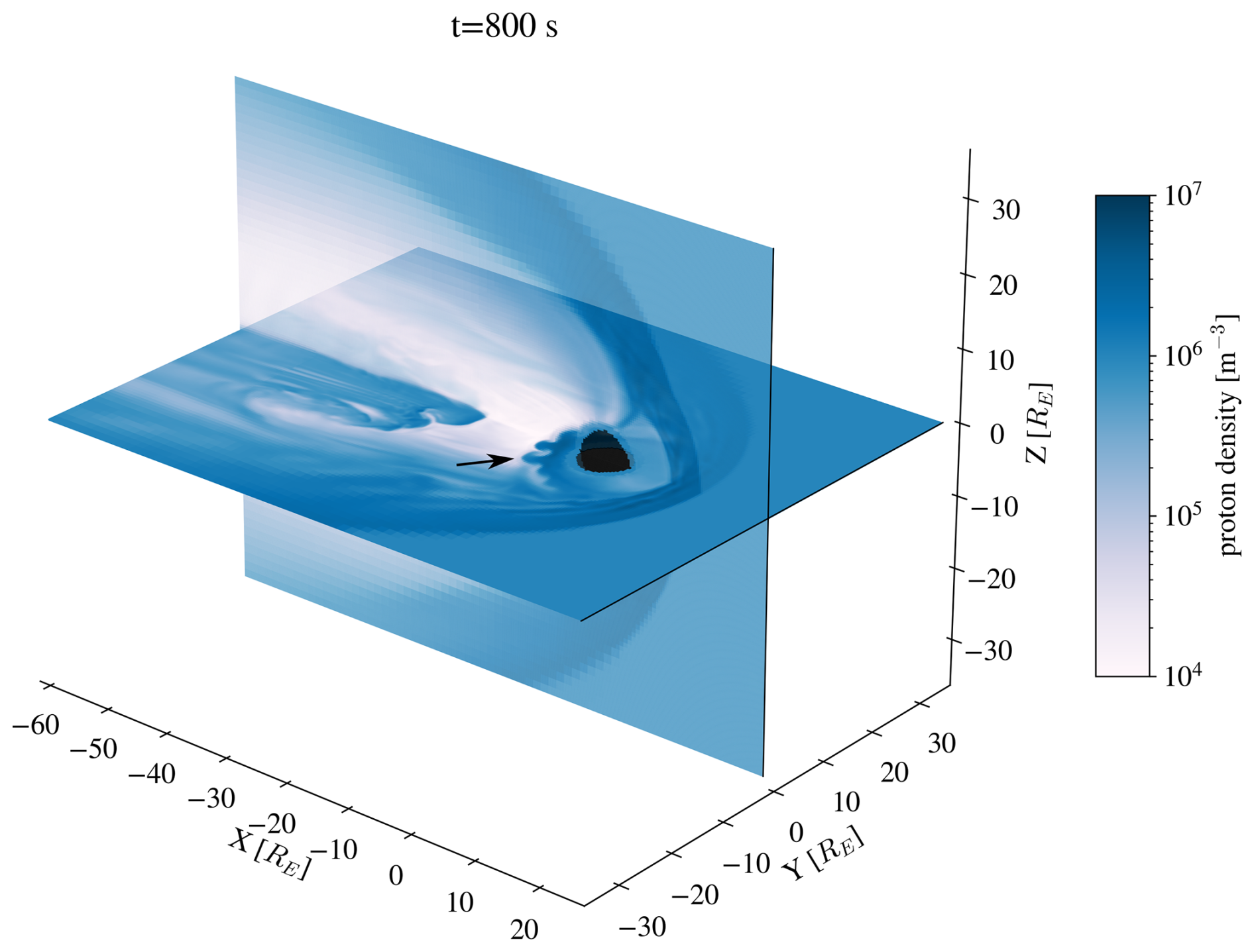
Figure 1 Part of the Vlasiator simulation domain, Y=0 and Z=0 planes, the axes are given in R_E. The colours show the proton density in the solar wind and magnetosphere at t=800 s. The simulation used GSE coordinates, with positive X directed towards the Sun. The solar wind enters the simulation box from the +X boundary, and flows in the −X direction. The vortex structure studied in this paper is indicated with an arrow on the nightside.

The recent addition of an ionospheric boundary model to Vlasiator (Ganse et al., 2025) allows us to investigate magnetosphere-ionosphere interactions. With the new addition to the model, the magnetosphere is now electrostatically coupled to the ionosphere with a strategy analogous to MHD simulations (e.g., Janhunen et al., 2012; Goodman, 1995). In the new approach, simulation conditions are fed from the magnetospheric domain to the spherical ionospheric grid through magnetic field lines, using a dipole field within the inner boundary of the simulation. The ionospheric boundary model is height-integrated, with all parameters integrated from ground level to an altitude of 200 km. The input parameters for the ionospheric model are FAC density j_∥, electron density n_e and temperature T_e, which are determined close to the inner boundary of the magnetospheric domain. Ampère's law, in the form $\mathit{j}=\text{curl}\mathit{B}/{\mathit{\mu }}_{\mathrm{0}}$ (analogous to the Curlometer technique in space craft data), is used to determine the current density j. The divergence of the three dimensional current density j then yields FAC density j_∥, which is given as input to the ionospheric solver. In the ionospheric solver, the FAC density is used to determine ionospheric surface currents and electric potential (Eq. 18 in Ganse et al., 2025). The details of the ionospheric boundary model are given in Ganse et al. (2025).

In the magnetosphere, the computational costs of running the simulation are alleviated by the use of adaptive mesh refinement (AMR). In the run used for this study, the spatial resolution was 8000 km at the lowest, with three steps of refinement applied to certain parts of the grid, resulting in 1000 km as the highest spatial resolution. The highest resolution is applied to the magnetotail current sheet. The simulation uses the GSE coordinate system. In the simulation there is no tilt to the Earth's dipole magnetic field, and so the dipole axis is aligned with the Z axis. The solar wind conditions for the simulation are given by the constant boundary conditions at the +X side of the simulation box. For the run discussed in this study, the solar wind speed was set to be constant at 750 km s⁻¹ towards the −X direction. The interplanetary magnetic field (IMF) was defined to be purely in the −Z direction with a magnitude of 5 nT. The density of the solar wind was set at 1 cm⁻³ and the temperature at 0.5 MK. The full duration of the run was 1612 s, with output generated at 1 s intervals. The size of the simulation box is from −110 to 50 R_E in the X direction and from −58 to 58 R_E in the Y and Z directions. In this run, protons are the only ion species.

3 Results

3.1 Overview of flow channel formation

The event begins with magnetic reconnection starting on the duskward (Y>0) transition region of the magnetotail at $X\sim -\mathrm{10}{R}_{\mathrm{E}}$ and Y∼7 R_E. As the simulation progresses, reconnection is initiated on the dawn side (Y<0) of the magnetotail as well. This can be seen in Fig. 2, which shows zoomed in sections of the Z=0 plane in the nightside tail. Due to flapping motion of the current sheet, the Z=0 plane may not exactly coincide with the current sheet, though this close to the Earth the flapping motion is not strong. We can thus study relevant dynamics by looking at this plane, which is close to the magnetotail current sheet. Figure 2 shows proton density, proton velocity v_x, magnetic field B_z, electric field E_y, pressure, and FACs at four time steps during the simulation. The FACs are shown as a function of magnetic local time (MLT) and geomagnetic latitude on the ionospheric grid of the simulation. The grey/pink contours on the magnetospheric figures mark ±400 km s⁻¹ ion velocities. Video S1 in the Supplement shows an animation of the proton density, v_x, and the FACs between t=580 and t=880 s.

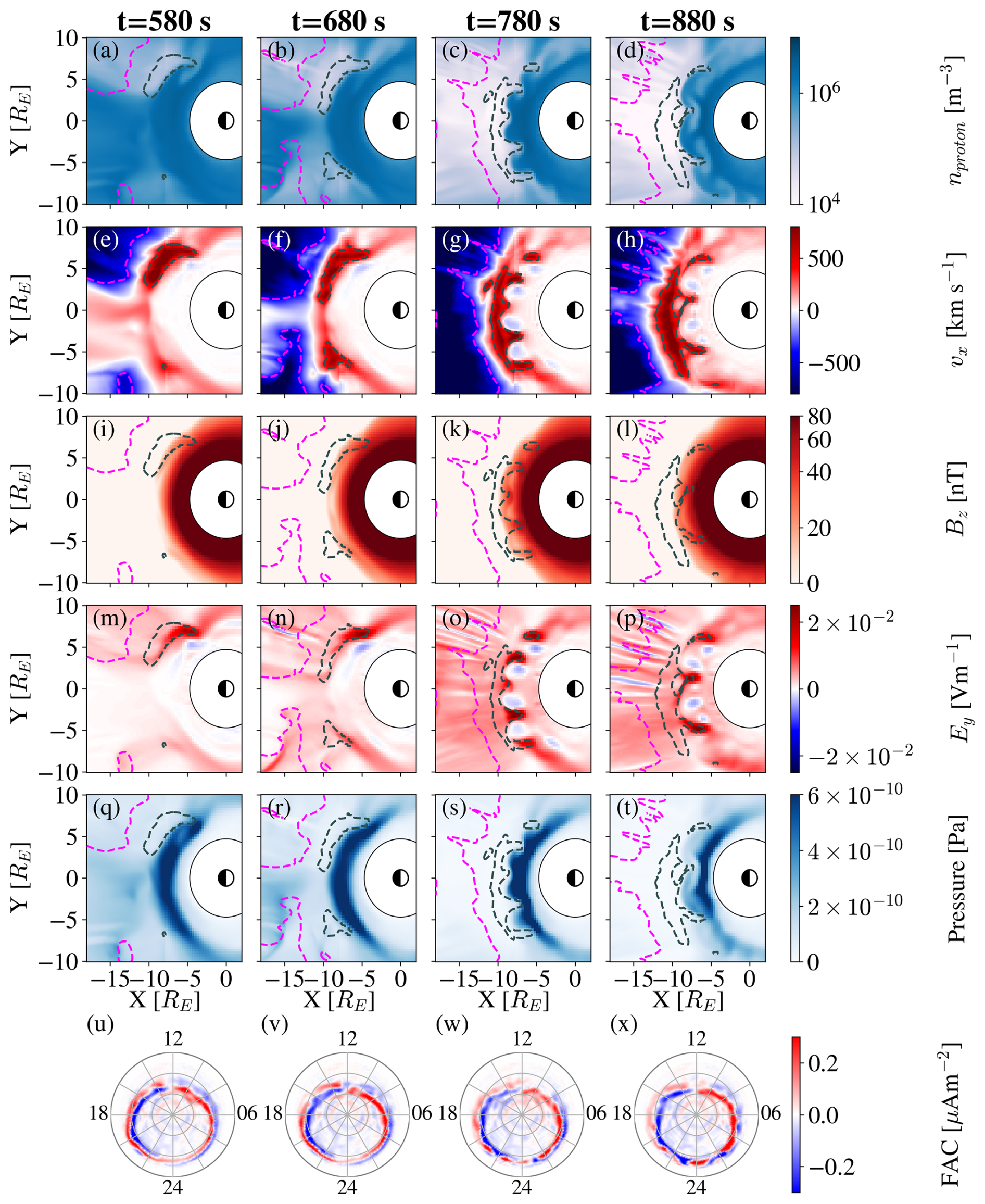
Figure 2 The evolution of the flows in the magnetosphere Z=0 plane and the ionosphere for four times in the simulation, with the columns each showing one time. Panels (a–d): proton density. Panels (e–h): ion v_x. Panels (i–l): B_z, Panels (m–p): E_y. Panels (q–t): pressure. The contour lines indicate 400 km s⁻¹ (grey) and −400 km s⁻¹ (pink) velocities. Panels (u–x): FACs on the ionospheric grid of the simulation, as a function of MLT and geomagnetic latitude, with red signifying current flowing into the ionosphere, and blue meaning current out of the ionosphere.

Figure 2a and b show a decrease in density, first on the dusk side, and then on the dawn side. At the same time, panels (e) and (f) show a region of strong Earthward flow, coinciding with the start of reconnection. The peak values of v_x are approximately 600 km s⁻¹, clearly exceeding the BBF threshold 400 km s⁻¹, and they coincide with the regions where density is lower. The reconnection starting on the western/dusk side of the magnetotail is possibly due to Hall effects causing favourable conditions for reconnection, as has been observed in previous hybrid simulation studies (Lin et al., 2014; Lu et al., 2016). The resolution of the simulation is also lower at the flanks of the magnetotail compared to the rest of the magnetotail, which likely plays a role in the initiation of reconnection, as will be discussed further in Sect. 4. As the magnetotail current sheet thins, ions become decoupled from the magnetic field. At the same time, a Hall electric field (not shown in the figure) forms in the Z direction (towards the neutral plane, B_x=0), which causes plasma to drift towards dawn. This results in a thinning of the current sheet on the dusk side, making it more prone to reconnection (Lu et al., 2016).

The formation of the flow channels is closely related to the spreading of the reconnection across the magnetotail. The X line can be seen in Fig. 2f at t=680 s as a flow reversal of Earthward/tailward flow forms at about $X=-\mathrm{12}{R}_{\mathrm{E}}$. This X line provides continuous driving of fast Earthward flow across the magnetotail throughout the event. Density undulations and narrow Earthward flow channels form in the transition region, as seen in panels 2c–d (density) and g–h (v_x). As the flow propagates closer to Earth, rebound flow in the tailward direction (v_x<0) is created. Additionally, the flow braking induces vorticity, which will be discussed more in Sect. 3.3. At the last time step, t=880 s, shown in Fig. 2d the density structure has dissolved into a mushroom-shaped pattern, which grows in spatial scale but diminishes in density. In the corresponding v_x plot (panel 2h) we observe that rebound flows on smaller scales (compared to panel 2g) begin to form.

Panels 2i–l show that the Earth's dipole field dominates the magnetic field z-component. At t=780 s (Fig. 2k), we see that the magnetic field B_z is enhanced in the regions where the fast plasma flows (grey curves) are decelerated in the transition region. The B_z enhancement is linked to dipolarization, a process influenced by the transport of magnetic flux through Earthward flows produced during reconnection. This dipolarization is also seen in Figs. 4 and 5, which will be discussed in the next section. Panels 2m–p in Fig. 2 show E_y, which is positive for regions of Earthward flow, corresponding with the idea of polarization leading to enhanced electric fields (Pontius and Wolf, 1990). The electric field pattern, with positive and negative E_y, is similar to the v_x structure in terms of Earthward flow being associated with positive E_y, and vice versa. This suggests that the convective electric field is a major part of the total electric field. Panels 2q–t in Fig. 2 show that pressure is increased on the Earthward side of the fast flows. In Panels 2s and t it can be seen that the contours of the fast flow match the structure of the increased pressure. At the last time step (panel 2t) the pressure has started to decrease considerably.

At t=580 s, it can be seen in panel 2u that the FAC structure (with red signifying current flowing into the ionosphere, and blue signifying current flowing out of the ionosphere) generally resembles the traditional picture of the R1 and R2 currents. At this time, in the dusk side an additional upward current is created between 20:00 and 22:00 MLT. At t=680 s in panel 2v the current patterns remain similar to the start of the event. In the last two panels (2w and x) large-scale patches of FAC structures form between 20:00 and 04:00 MLT. It can be seen that the original clear R1 and R2 current pattern starts to shift into a patchy distribution, where the boundary between downward and upward currents becomes wavy. The current flowing into the ionosphere intensifies, going from a maximum of ∼0.5 µA m⁻² at t=580 s to a maximum of ∼0.7 µA m⁻² at t=780 s. After this the inflowing current starts to become weaker again. The maximum values of outflowing current do not follow the same trend, but are higher at the start and end of the event (∼0.76 µA m⁻² at t=580 s, ∼0.84 µA m⁻² at t=880 s) and lower for the the times in the middle (∼0.67 µA m⁻² at t=680 s, ∼0.69 µA m⁻² at t=780 s). Between t=780 s (panel 2w) and t=880 s (panel 2x) the areas of the FAC patches grow. The change in FAC structures is seen predominantly at lower latitudes on the equatorward edge of the current structure. The connection between the FACs and the fast flows is explored in more detail in Sect. 3.3.

As for the scales of the flow, in the magnetosphere the wavelength (defined as the distance between the plasma density maxima at a radial distance of ∼8 R_E) of the vortices is about 3.5 R_E prior to the “mushroom”-like dissipation. In the ionosphere, the wavelength of the FAC structures is about 1000 km. The way the density variations evolve closely resembles the behaviour expected from the Rayleigh-Taylor instability and its plasma analogue, the ballooning/interchange instability, which will be discussed in more detail in Sect. 3.2.

Figure 3 shows the flow structures in the YZ plane at $X=-\mathrm{8}{R}_{\mathrm{E}}$ at t=790 s, when they are at their clearest before they start decaying. At this distance in the tail, the size of the structures is about 3 R_E in the Z direction. Positive v_x (panel 3a) and positive E_y (panel 3b) correlate with each other within the structures. In the magnetic field z-component (panel 3c) we see an increase in the regions where the bulk flow is directed towards the Earth (v_x>0) and a decrease when the flow is directed towards the tail (v_x<0). This implies a buildup of magnetic flux at the leading edge of the Earthward flows.

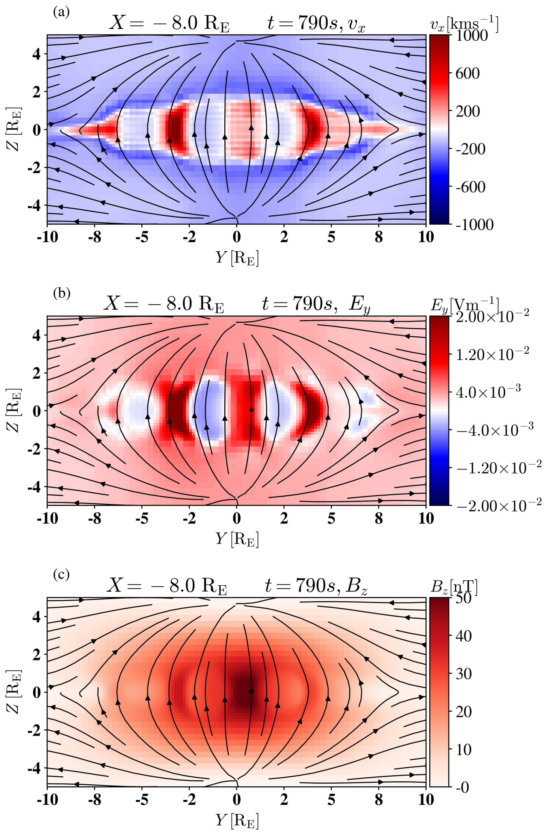
Figure 3 The transition region structures from the nightside magnetotail at $X=-\mathrm{8}{R}_{\mathrm{E}}$ at t=790 s. The black curves show the magnetic field lines in the plane. Panel (a) shows v_x, panel (b) E_y, and panel (c) B_z.

3.2 Signatures of the ballooning/interchange instability

As mentioned in Sect. 3.1, the evolution of the density gradient at the transition region closely resembles the fluid Rayleigh-Taylor instability, whose equivalent in a curved magnetic field plasma is the ballooning/interchange instability. In the magnetotail the instability can be studied through analysis of B_z and entropy S gradients, and changes in pressure P, as was done by e.g. Sorathia et al. (2020) and Birn et al. (2009). The ballooning/interchange instability is governed by plasma pressure and the curvature of the magnetic field. Accumulation of the magnetic flux in the tail lobes leads to stretching of the current sheet which leads to an increase of the curvature of the magnetic field in the near-Earth region, making it prone to ballooning. Birn et al. (2009) found that the magnetotail is stable when pressure decreases monotonically towards the tail, while flux tube entropy increases. The entropy may decrease in the tail due to loss in either flux tube volume or pressure. One example of entropy loss is reconnection pinching off part of a flux tube, thus decreasing its volume. Particle precipitation may also play a role in entropy loss, but it is not expected to be significant compared to magnetospheric sources of loss (Wolf et al., 2009). In summary, it is expected that a radially non-uniform entropy profile in the tail direction may cause loss of equilibrium.

Figure 4 shows the z-component of the residual magnetic field ΔB, defined here as the difference between the initial magnetic field (dipole field and constant IMF) at the start of the simulation, and the magnetic field at a particular time step. A decrease in equatorial B_z signifies an increase in magnetic field curvature. Additionally, we plot the flux tube entropy S for the same times as in Fig. 2. The flux tube entropy is calculated as an integral over closed magnetic field lines, which is why parts of the figure are empty (white), in the regions where the field lines are open. The dashed line at Y=0 shows the line along which the radial profiles of S and B_z will be shown in Fig. 5. At the start of the event, most of the transition region exhibits a decrease in B_z, consistent with the stretched field lines prior to the onset of reconnection. At the Earthward flows (t=780 s), B_z can be seen to increase from negative values towards zero, as seen in panel 4a on the dusk side. As the simulation progresses, there is a similar increase in B_z along the Earthward edge of the fast flow region, especially clear in panels 4c and d.

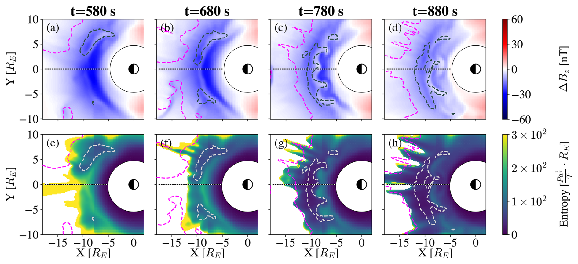
Figure 4 Panels (a–d): Residual B_z, i.e. the magnetic field minus the Earth's dipole field (ΔB_z). Panels (e–h): flux tube entropy S. All panels are in the Z=0 plane, with ±400 km s⁻¹ velocities marked with grey/pink contours. The four time steps are the same as in Fig. 2. The dashed line at Y=0 is the line that is shown as a radial profile in Fig. 5.

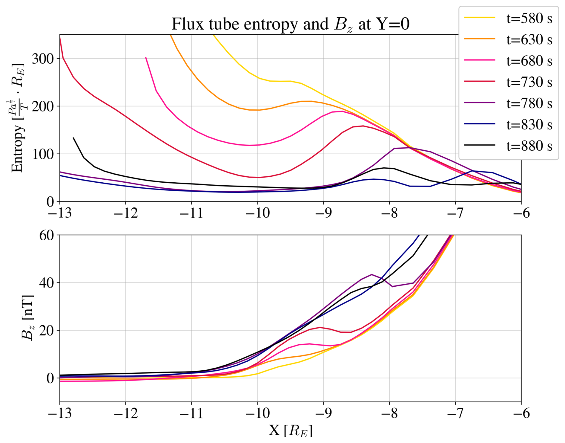
Figure 5 The radial profiles of flux tube entropy and B_z at Y=0. The flux tube entropy is calculated along closed magnetic field lines. Note that the resolution of the simulation changes at $\sim -\mathrm{8}{R}_{\mathrm{E}}$, Earthward of this point the resolution is lower.

Figure 4a and e show that the entropy is decreased in the regions where there is Earthward flow and an increase in residual B_z, such as the fast flow region on the dusk side. Comparing to Fig. 2, these are also the regions of low density. In regions of high pressure (Fig. 2), the flux tube entropy S is also high, as is expected by the definition of S. At time steps t=780 and t=880 s (panels 4g and h) there is a clear drop in entropy that coincides with the regions of fast flow. The wavy structure that forms from high values of entropy (most clearly in panel 4g) mirrors the regions of high pressure and high density.

Similarly to the previous figures (Fig. 2, panels showing t=780 s) of the same plane, by visual inspection we see that the wavelength of the structure is about 3.5 R_E. While there is slight variation in the scales of the Earthward flows and corresponding entropy depletion, this almost periodic structure is an indication of a plasma instability. The wavelength grows in the timescale of about 100 s, from t=680 to t=780 s. This is the period where the transition region goes from no wave-like structure to the maximum wavelength before the nonlinear effects start to dominate (after t∼800 s), and the structure starts to diffuse. The wavelength of the structure is likely defined by the scales of the first Earthward BBF flows at dawn and dusk, similarly to the studies by Guzdar et al. (2010); Lu et al. (2013). However, it is difficult to distinguish the factors controlling the instability scales, as the magnetotail exhibits both BBF-like flows and a tailwide entropy depletion.

As mentioned, the non-uniform growth of flux tube entropy towards the tail is an indicator of the ballooning/interchange instability (e.g., Birn et al., 2009; Wolf et al., 2009). For a stable state, the flux tube entropy would be expected to uniformly increase with distance from Earth towards the tail. The formation of a “dip” in the radial entropy profile as time progresses is an indication of possible instability. We study this by plotting the radial profiles of flux tube entropy and B_z at Y=0, which is representative of the tail dynamics. The results are shown in Fig. 5, with profiles given every 50 s from t=580 to t=880 s. Note that the refinement level in the magnetotail decreases Earthward of −8 R_E. The dashed line in Fig. 4 shows the line along which the profile is taken. There is a clear, spatially localised, decrease in flux tube entropy at $\sim -\mathrm{10}{R}_{\mathrm{E}}$ as the simulation progresses, corresponding to a change in the B_z profile. At the radial distance where entropy starts to decrease, a local minimum develops in B_z due to dipolarization further in the tail. A B_z “hump” forms in the magnetic field profiles. This is seen, for example, for t=730 s (red curve) as an increase of B_z between at $X\sim -\mathrm{10}{R}_{\mathrm{E}}$ and $X\sim -\mathrm{9}{R}_{\mathrm{E}}$ and a minimum at $\sim -\mathrm{8.7}{R}_{\mathrm{E}}$. At this time, we see a tailward B_z gradient and an Earthward S gradient, indicating instability (Birn et al., 2018). The decrease of entropy and dipolarisation in B_z profiles are evident for the times from t=680 to t=780 s, as entropy in the tail decreases with time. After this, at t=830 s the entropy in the transition region is lower than at t=880 s. This is due to the wavy interchange structure increasing in azimuthal size, so that a higher entropy region moves to Y=0 by 880 s. This is seen in Fig. 4g and h, when looking along the Y=0 R_E line. At t=780 s Y=0 is between two regions of higher entropy at the transition region ($X\sim -\mathrm{10}{R}_{\mathrm{E}}$). By 880 s, the maximum entropy value has decreased, but the high entropy regions have increased in size, so at Y=0 R_E, $X=-\mathrm{10}{R}_{\mathrm{E}}$ we see a slight increase in entropy. We remind the reader that Fig. 5 shows the full B_z values, while Fig. 4 shows the residual B_z. Thus, the numerical values from Fig. 5 should be compared to panels i–l in Fig. 2 rather than to Fig. 4.

The reduction of entropy can be attributed to reconnection and the loss in density and flux tube volume that is related to the plasmoid released in the tailward direction. This could also be the case in our simulation, where we see a decrease in entropy in regions where reconnection is triggered and density decreases. The fact that we see a decrease in entropy corresponding to the first Earthward flow that starts the event implies that the flow region is ballooning unstable (Birn et al., 2009).

The ballooning/interchange instability is thought to induce density variations, such as the ones in Fig. 2, and the motion and stretching of magnetic field lines, for several different modes of the instability (e.g., Lin et al., 2014; Birn et al., 2015; Sorathia et al., 2020). To study this, we follow the motion of selected field lines. We choose 8 field lines with their original seed points at the Z=0 plane, and track the motion of their magnetospheric foot points as the simulation progresses. This is shown in Fig. 6, where field line placement is shown for three times (from t=775 to t=815 s) in the simulation. The colouring of the lines has no physical significance and is used simply to track the motion of the lines in relation to each other. The field line motion is shown against the magnetotail current sheet, where we plot the x-component of velocity. At t=775 s the field lines are grouped in two rows but as the simulation progresses they start to change position relative to each other. There is motion both in the X and Y directions, and we see that the green lines (initially at larger Y values) and the blue/purple (grouped initially at smaller Y) change positions relative to each other. Between t=795 and t=815 s there is also radial drift, where the outermost purple field line drifts further from the Earth, while the other lines drift closer to the Earth.

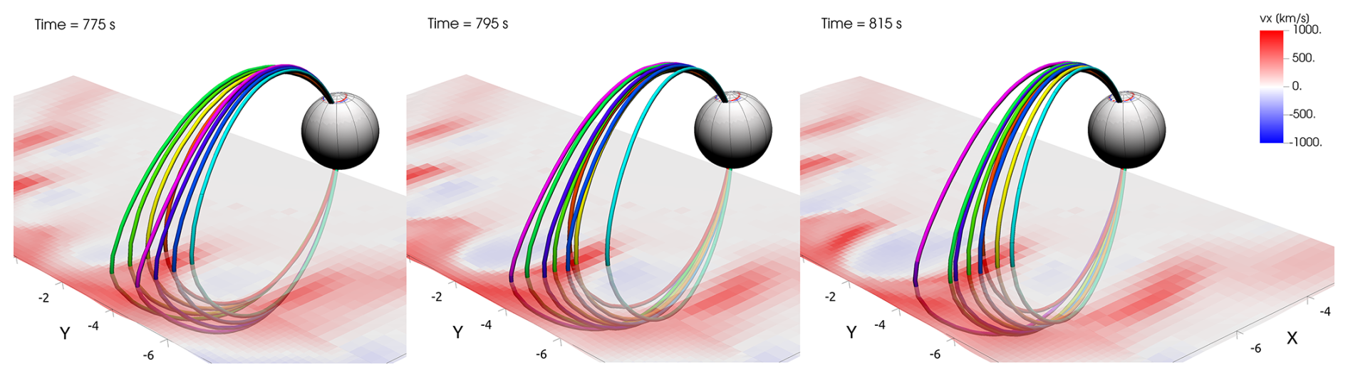
Figure 6 A zoomed in section of the magnetotail, where we trace selected field lines on the current sheet plane as the simulation progresses. The colours are used to distinguish the field lines from each other. The colormap shows the x-component of velocity in the magnetotail current sheet (where B_x=0). The axes are in R_E.

In summary, we found that there is clear variation in flux tube entropy in the magnetotail, in the X and Y directions, coinciding with regions of fast flow. The event begins with a tailwide depletion in flux tube entropy, indicating that the tail is unstable to the ballooning-interchange instability. Additionally we studied the motion of the magnetic field lines, and found interchange motion of field lines, though mostly in the Y direction. These findings indicate that the structures in e.g. velocity and density are due to the ballooning-interchange instability.

3.3 Ionosphere-magnetosphere coupling and dynamics of fast flows

Finally, to investigate the effects of the fast flows, along with coupling between the magnetospheric and ionospheric domains, we plot the ion velocity v_x and the vorticity on the magnetotail current sheet (∇×V)_z and study how they connect to the FACs in the ionosphere.

The coloured regions in Fig. 7a show v_x, while plasma motion in the current sheet is indicated with the black arrows. In Fig. 7b the colours indicate the z-component of vorticity. To find where the field lines from points of high vorticity map to, we plot the ionospheric grid in Fig. 7c. Comparing Figs. 7a and b, we see that the regions of high vorticity are located at the flanks of the Earthward flow channels. Thus it would appear that the Earthward flow induces vorticity in the transition region. Following the field lines, counter-clockwise (positive vorticity) plasma motion in the current sheet corresponds to FACs flowing away from the ionosphere (blue colour in the figure), and vice versa. The FAC flow that is associated with each Earthward flow channel is oriented in the R1 sense in terms of direction of the current, as is to be expected based on the literature (e.g. Birn et al., 2004; Yu et al., 2017). The change to FACs is seen mostly in the R2 region, meaning the pair of FACs at lower latitudes.

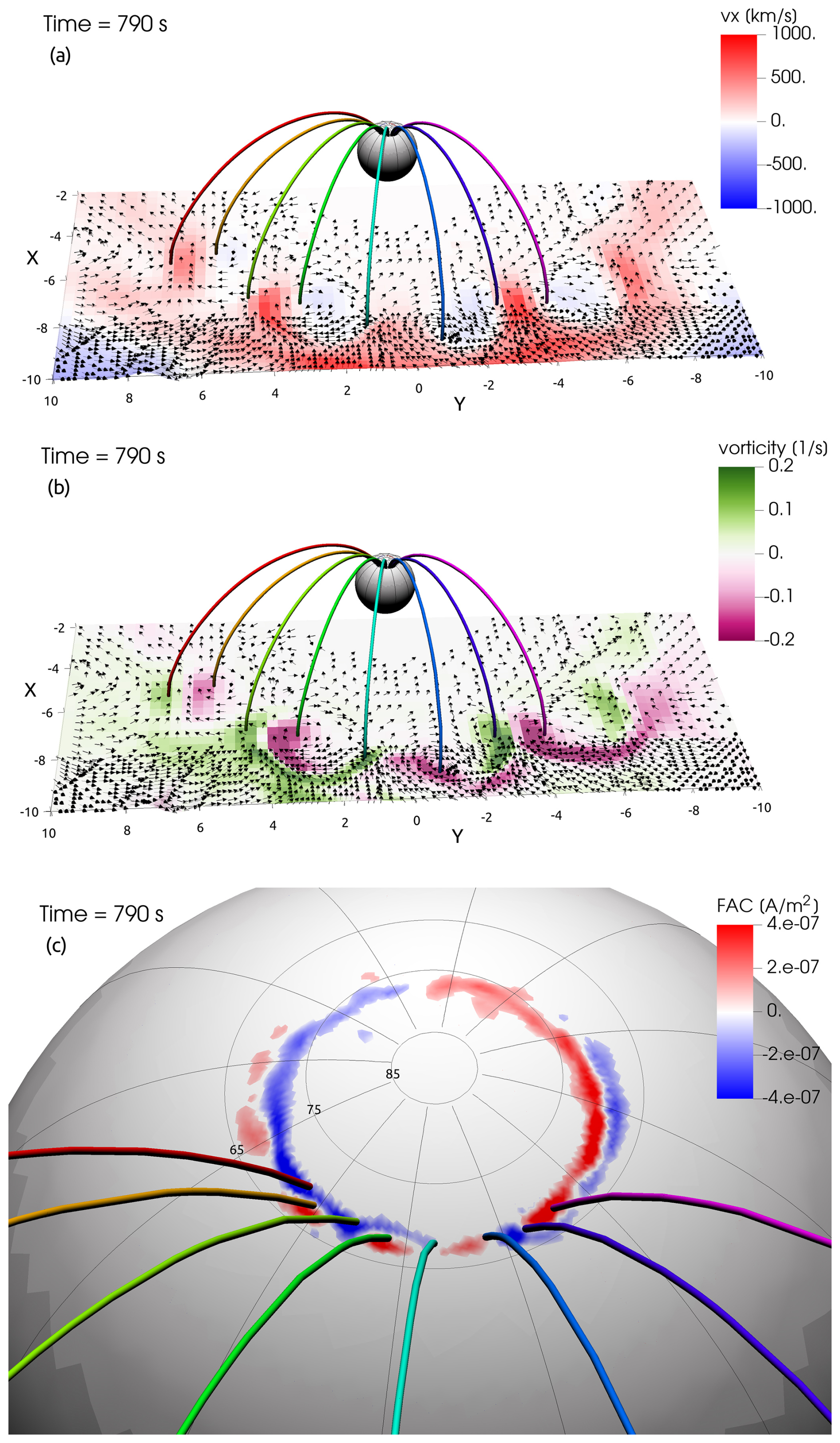
Figure 7 The coupling of magnetic field lines to the ionospheric grid. Panel (a) shows the velocity x-component in the current sheet (B_x=0). The arrows point to the direction of the plasma velocity in the current sheet. The colouring of the traced field lines has no physical meaning. The axes units are in R_E. Panel (b) shows via the colormap the vorticity of bulk flow (∇×V)_z on the current sheet. Panel (c) is a zoomed-in section of the ionospheric grid, where the same field lines as in panels (a) and (b) can be seen to map to the ionosphere. Here the colormap shows FAC strength.

From these figures we see that in addition to the ballooning/interchange instability discussed in the previous section, the dynamics of the fast flows also play a key role, at least in creating the FAC structure seen in the ionosphere.

4 Discussion

In our simulation we have observed the formation and evolution of structured fast Earthward flow channels that create vorticity and FACs coupling to the ionosphere. The wavelength of the vortex flow in the transition region is about 3.5 R_E, and 1000 km in the ionosphere. In the previous literature, similar Earthward flows and the ballooning/interchange instability have been studied in a variety of simulation and observational studies. The conditions and features of the instability and the resulting ionospheric and magnetospheric signatures vary between the different simulation/observation approaches. The event, i.e. the creation of vortex flow, observed in our simulation shares features similar to many previous studies, but also presents distinct differences. Using the hybrid-Vlasov approach, we can self-consistently model the current sheet thinning, reconnection, and loss of flux tube entropy in the magnetotail, which sets the stage for the development of the instability. These phenomena are also mapped to the ionosphere, and reflected in the FAC structure we observe there. Thus we are combining the findings of previous research to offer an explanation for the development of several flow channels in the near-Earth magnetotail. We summarize below previous key studies to place our findings in context.

The event seen in our ion-kinetic simulation most closely matches the spatial scales seen in MHD and RCM simulations of low-entropy Earthward flows. Sazykin et al. (2002); Yang et al. (2008); Sun et al. (2021) studied a case where a wide low-entropy front was injected into the RCM simulation domain, which then broke into smaller channels of Earthward flow. In our simulation a similar region develops self-consistently as a result of reconnection spreading across the magnetotail. The initial lowering of entropy as a result of reconnection at dawn and dusk is similar to the MHD studies discussed in the next paragraph, but due to kinetic effects, the reconnection spreads over the magnetotail, resulting in a wide region of Earthward flow that corresponds to an entropy decrease.

The changes in the profiles of flux tube entropy S and magnetic field B_z we see (Fig. 5) are similar to the study of MHD stability of B_z minima by Birn et al. (2018). The authors found that B_z hump configurations can become unstable if the pressure is sufficiently low and there is a corresponding entropy decrease. This is the case in our simulation. Additionally, Birn and Hesse (2013) studied the substorm current wedge in relation to Earthward-propagating low-entropy bubbles. They found Earthward flows that break into narrow channels, which resulted in azimuthally spread ionospheric signatures, similar to our study. They speculated that this effect is a combination of a cross-tail mode such as the ballooning/interchange, in combination with reconnection spreading over the night side. This scenario is supported by our simulation, with the event being driven by tailwide flow that is unstable to ballooning/interchange.

Guzdar et al. (2010) and Lu et al. (2013) studied the interchange instability in 2D MHD, aiming to model the creation of multiple dipolarization fronts. They used a seed perturbation of the BBF scale (1–3 R_E) to initiate the instability, and found that the scale of this initial perturbation controlled the scale of the resulting wavelength of the instability. Lapenta and Bettarini (2011) used a 3D MHD simulation to find self-consistent seeding of interchange instability in dipolarization fronts, following magnetic reconnection which was related to the kink instability. The scale of the kink instability determined the scale of the structures formed by the interchange instability. The results from these studies resemble our case in the sense that the wavelength of the azimuthal perturbation is comparable with the size of fast flow channel generated by the first burst of reconnection. The multiple dipolarization fronts are similar to the azimuthal structure we observe. In terms of observations, there have been THEMIS satellite observations of a wavy dipolarization front, studied by Wu et al. (2018).

More recently, Sorathia et al. (2020) studied the ballooning/interchange instability in a substorm growth phase. The spatial scales seen in their study (4000 km in the magnetosphere) were much smaller than in previous MHD studies. The analysis we do in Fig. 4 is similar to that done by Sorathia et al. (2020), though the magnetospheric conditions for the rise of the instability are different between our study and theirs. Conversely to the previously mentioned MHD studies, the initiation of the instability in Sorathia et al. (2020) was not related to reconnection in the magnetotail, but arose from a tailward B_z gradient and a decrease in flux tube entropy. These conditions were due to the thinning of the current sheet due to magnetic flux moving to the dayside. The magnetospheric structures were mapped onto the ionospheric grid of the simulation, where the scales matched that of auroral beading. While the instability conditions (entropy and B_z gradients) are similar in our simulation, there is a key difference that possibly explains the difference in scales between the two studies. Our simulated event is driven by fast flows that result from reconnection, while their simulation focuses on the substorm growth phase and the thinning magnetotail current sheet, prior to reconnection onset.

Xing et al. (2013) used a conjunction of spacecraft and THEMIS all sky imagers to study the auroral response to the ballooning/interchange instability. They found evidence of the instability initiated at $X=-\mathrm{11}{R}_{\mathrm{E}}$ in the magnetotail, with a wavelength of 1–3 R_E. The auroral response to this was the creation of additional wavelike structures on preexisting auroral arcs. These scales are similar to what we see in our simulation. Xing et al. (2020) continued this work and suggested that the ballooning/interchange instability resulted in auroral wave structures, but did not necessarily lead to substorm onsets.

The auroral response to the ballooning/interchange instability is often thought to be auroral beading, i.e. an auroral form consisting of azimuthally separated auroral patches (e.g., Motoba et al., 2012). The ionospheric scales of these auroral beading events are smaller than what we observe in our simulation. Nishimura et al. (2022) used THEMIS all sky imagers and satellites, and found that the beading events studied matched the scales of e.g. the simulations by Sorathia et al. (2020). The magnetospheric data from THEMIS indicated that ballooning/interchange was a possible candidate for the creation of the auroral beading. Conversely, Ohtani and Motoba (2023) found that auroral beading should be attributed to a process on a smaller scale than the ballooning/interchange instability, and that mesoscale or large scale convection could not control auroral beading.

As for the drivers of the vortex flow in our simulation, magnetic reconnection appears to play a key role in the development of the instability and determining its observed scale. Reconnection occurs in the Vlasiator simulation due to numerical resistivity. In the simulation studied here, reconnection is initiated at the dawn and dusk flanks and then spreads across the magnetotail. This behaviour could result from the flanks having a coarser simulation grid and consequently relatively higher numerical diffusion compared to the midnight region. The reconnection eventually leads to an entropy depletion, which then creates an azimuthally symmetric, wave-like structure, evident e.g. in density (Fig. 2c). As the simulation progresses, this wave-like structure extends from the lower resolution to the higher with the same wavelength in both regions. Very-near-Earth reconnection (at a distance of <14 R_E from Earth) is found to be statistically rare, but occurring at times of high dynamic pressure when the magnetotail becomes compressed (Beyene and Angelopoulos, 2024). The initiation of the reconnection on the dusk side of the magnetotail agrees with previous hybrid simulations (Lin et al., 2014; Lu et al., 2016), where Hall effects were causing favourable conditions for reconnection primarily at the dusk. A Hall field is induced also in our simulation, but it is not shown in the figures. These factors suggest that the combination of the resolution and the physical effects sets the conditions for the onset of reconnection.

The creation of the vortex flows occurs at an early stage in the simulation run, where the magnetosphere is still in its phase of global reconfiguration caused by tail reconnection. The R1 and R2 field-aligned current systems have already formed by this point in the simulation, and so we can study the current closure in the ionosphere. This marks the first large-scale reconnection event seen in the simulation run. Due to the early state of the simulation, the magneotail is very elongated. This period of initialisation is followed by rapid reconfiguration of the magnetotail due to large-scale reconnection. Such a situation could potentially arise when a period of slow solar wind is followed by very fast solar wind, triggering large-scale reconnection.

The balance between fast flows creating vorticity and the ballooning/interchange creating a similar structure is an interesting matter. While the Earthward flow is arguably an important driver of the observed structures, causing rebound flows and vorticity, our results suggest that the ballooning/interchange instability also plays a role. As mentioned, we observe a tailwide depletion of flux tube entropy. The decrease in entropy with increasing radial distance from Earth (Figs. 4 and 5) is indicative of instability to the ballooning/interchange. Additionally, later in the simulation we observe the interchange motion of the field lines (Fig. 6). We see the field lines moving in both X and Y directions. The emergence of “mushroom-like” density structures (Fig. 2d) is also an indicator of an instability, visually resembling the Rayleigh-Taylor fluid instability. It appears that the Earthward flow seeds the instability similarly to the studies by Guzdar et al. (2010), Lu et al. (2013).

Another factor to be considered is the effect of the ionospheric boundary model on the creation of the vortex flows. The current Vlasiator ionospheric boundary allows field lines to move in the ionosphere. This enables the observed field line motion, and allows for the creation of vorticity. Studying the effects of the ionospheric boundary in more detail could be beneficial: For instance, it would let us see how the conductivities affect global magnetospheric convection. It would seem that in this case the reconnection in the magnetotail is the main driver of the instability rather than e.g. the ionospheric conductivity model. This is because the creation of the vortex flow coincides with the initial sites of reconnection in the magnetosphere.

The observed scales we see in the magnetosphere match those of BBFs, similar to e.g. Birn et al. (2011). Figure 7 shows the mapping of field lines from the current sheet onto the ionospheric grid, where it can be seen that the FAC pattern is created in the typical R1 sense that is associated with BBF-like flow. In the ionosphere, the scales (∼1000 km) most closely match those of substorm wedgelets, similarly to Nishimura et al. (2020) who surveyed substorms with wedgelet type current loops, and found the average size of the wedgelets was found to be ∼3.2 R_E in the azimuthal direction in the magnetosphere and ∼600 km in the ionosphere. Thus, this type of vortex flow creation is a possible explanation for the FAC “wedgelet” phenomenon, where several pairs of FACs are observed in the ionosphere, spread across a wide range of longitudes. In our results we see the transition from a the classic R1/R2 ionospheric current pattern (before the large inflow region splits into several flow channels, t=680 s) to a “wedgelet” type current distribution, associated with multiple magnetospheric flow channels, at t=780 s.

5 Conclusions

In this paper we study the appearance of large-scale vortex flow in the transition region between the dipole field and the magnetotail in a global hybrid-Vlasov simulation. The main finding of the paper is as follows: The vortex flow channels in the transition region are triggered by magnetic reconnection, which results in plasma motion both Earthward and towards the magnetotail. The fast Earthward plasma motion coincides with a flux tube entropy depletion. This enables the growth of the ballooning/interchange instability, causing the Earthward flow region to split into several BBF-like flow channels. We compare the results from our study to previous simulations, and find that the spatial scales and features of the flows mostly match MHD and RCM results where the ballooning/interchange instability is initiated by reconnection and a depletion of entropy in the magnetotail.

The event seen in our simulation begins with the thinning of the magnetotail current sheet followed by continuous tailwide magnetic reconnection. The Earthward flow splits into several flow channels, which have similar properties to BBFs, and create additional FACs in the R1 sense. This means current flowing into the ionosphere on the dawn side of the flow channel, and current flowing out of the ionosphere on the dusk side. The width of the Earthward flow intrusions is ∼3.5 R_E, and they coincide with a decrease in flux tube entropy and an increase in residual B_z. The event shows properties of both BBF-related dipolarization and large-scale reconnection outflow from the tail-wide X line, and the ballooning/interchange instability.

As the magnetospheric solver of the simulation is coupled to an ionospheric solver, we can also study the ionospheric response to the Earthward flows and vorticity. In the ionosphere, we observe the FACs starting to deform to a patchy structure that coincides with the vorticity observed in the transition region. Our results expand on the previous literature on the connection between the dynamics of fast flows/BBFs in the near-Earth magnetotail, and the large-wavelength manifestations of the ballooning/interchange instability. We offer a possible explanation for the creation of multiple flow channels in the near-Earth magnetotail, and the formation of “wedgelet” type FAC patterns.