Magnetospheric convection in a hybrid-Vlasov simulation

The Dungey cycle is a fundamental process governing large-scale plasma dynamics in the near-Earth space, traditionally examined through Magnetohydrodynamic (MHD) simulations and ionospheric observations. However, MHD models often oversimplify the complexities of driving dynamics and kinetic processes, while observational data tend to lack sufficient coverage. In this study, we utilize a hybrid-Vlasov simulation to investigate the Dungey cycle, and introduce a novel method for quantifying reconnection voltages in different Magnetic Local Time (MLT) sectors. This method is validated by comparing it with the ionospheric open flux change rate in the simulation. Our analysis identifies discrete azimuthal convection channels of closed field lines, clearly initiated by dayside reconnection and propagating to the nightside. These channels are prominent even during intervals of intense nightside reconnection. Notably, we observe that the effective length of dayside reconnection fluctuates, even under steady solar wind conditions. Our results reveal significant deviations from MHD theory, which predicts that plasma flows within the magnetosphere should follow flux tube entropy isocontours. Instead, we demonstrate that plasma flows near reconnection sites and at the terminators deviate from isentropic behavior, suggesting the presence of non-adiabatic processes in these regions. This study validates the representation of the Dungey cycle in the Vlasiator 3D simulation and enhances our understanding of global plasma convection. Future work should focus on identifying the kinetic processes that explain the deviations in the plasma convection with flux tube entropy isocontours between MHD theory and kinetic approach.

1 Introduction

Magnetospheric convection is a fundamental topic in space plasma physics, which has been extensively studied over the years. For instance, Cowley (1982) reviewed and compared two primary mechanisms that drive convection in the Earth's magnetosphere: magnetic reconnection, originally proposed by Dungey (1961) and viscous-like interactions at the magnetopause boundary, introduced by Axford and Hines (1961). Axford (1969) discussed the impact of convection across the magnetosphere, highlighting its role in auroral formation, its influence on the size and dynamics of the plasmapause, and its contribution to particle acceleration. The pioneering contribution to understanding magnetospheric convection was introduced by Dungey (1961), who proposed that the motion of collisionless plasma is frozen-in to the field lines between dayside and nightside neutral lines of the Earth's magnetosphere. The plasma motion between these two lines is known as the Dungey cycle. Furthermore, Sergeev and Lennartsson (1988) concluded that steady magnetospheric convection (SMC) events, which are periods of enhanced magnetospheric convection activity, can occur during prolonged intervals of southward interplanetary magnetic field (IMF) without triggering substorms or disrupting the tail current.

The Dungey cycle begins when the southward IMF interacts with the Earth's northward magnetic field on the dayside magnetopause, triggering magnetic reconnection. This process opens previously closed magnetospheric field lines, allowing the newly opened field lines, along with the plasma particles frozen-in with them to be transported toward the nightside by the tailward-flowing solar wind. This magnetic flux is accumulated in the tail lobe region and leads to an increase of magnetic pressure. The pressure causes open field lines from the northern and southern hemispheres to converge at the tail current sheet, where reconnection occurs again, closing the field lines. The closed magnetic flux then migrates back to the dayside within the flank regions of the magnetosphere, completing the cycle. The footprints of this plasma convection in the magnetosphere form a twin-cell plasma convection pattern within the polar cap in the ionosphere. The entire convection process typically lasts for 2 to 5 h (Kennel, 1995). A similar convection pattern has also been discovered in other planets such as Mercury (Sun et al., 2020) and Saturn (Jackman and Cowley, 2006).

Siscoe and Huang (1985) proposed a formula to quantify the strength of the Dungey cycle by relating dayside and nightside reconnection voltages to the open flux change rate in the polar cap region:

$$\begin{array}{}\text{(1)}& \left|{\mathrm{\Phi }}_{\mathrm{D}}\right|-\left|{\mathrm{\Phi }}_{\mathrm{N}}\right|={\displaystyle \frac{\mathrm{d}{F}_{\mathrm{pc}}}{\mathrm{d}t}},\end{array}$$

where Φ_D(t),Φ_N(t) represent the reconnection voltages on dayside and nightside. F_PC denotes the amount of open flux in the ionosphere. The reconnection voltage in this context refers to the amount of magnetic flux transitioning between “open” and “closed” states per unit time. Holzer et al. (1986) proposed an empirical equation determining the dayside reconnection voltage:

$$\begin{array}{}\text{(2)}& {\mathrm{\Phi }}_{\mathrm{D}}=L_{\mathrm{eff}}\left|V_x\right|\left|B_z\right|,\text{for}{B}_z<\mathrm{0}\end{array}$$

In this formula, B_z is the z component of the IMF and V_x denotes the x-component of solar wind velocity. The axes are defined in the standard Geocentric Solar Magnetospheric (GSM) coordinate system. The term L_eff represents the effective length of dayside reconnection, ensuring the dimensional consistency of the equation.

The sunward directed convection described in the Dungey cycle is initiated by nightside reconnection. In addition to this, a distinct form of convection, driven exclusively by dayside reconnection, has also been extensively studied in recent years. For instance, Hsieh and Otto (2014, 2015) associated this dayside-driven convection with the formation of a thin current sheet in the near-Earth magnetotail, employing an ideal-MHD simulation within a spatially confined region. They introduced the concept of magnetic flux depletion, where dayside reconnection creates a magnetic flux erosion region in the dayside magnetosphere. To replenish this erosion, magnetic flux is depleted on the nightside and adiabatically convected sunward to restore equilibrium. Gordeev et al. (2017) demonstrated that the depletion of magnetic flux in the near-Earth tail region is directly related to the dayside reconnection using global MHD simulations. They revealed that the transport rate of magnetic flux in the near-Earth tail is proportional to the dayside merging rate. Dai et al. (2024) provided convincing evidence of dayside-driven convection, by tracing the progression of magnetospheric convection using keograms in global MHD simulations, supported by ionospheric observations. This type of convection is shown to establish within 10–20 min across the magnetosphere. Furthermore, they argued that this type of convection is related to the equatorward and dayside-to-nightside extent of field-aligned currents (FACs), emphasizing its relation to ionospheric dynamics (Zhu et al., 2024).

Previous research on the topic of magnetospheric convection has predominantly focused on ionospheric observations (Milan et al., 2007; Zhang et al., 2015; Milan et al., 2021; Gasparini et al., 2024) and MHD simulations (Gordeev et al., 2011; Dai et al., 2024). For instance, Milan et al. (2007) analyzed 25 nightside reconnection events using Eq. (1), utilizing global auroral images to determine the open-closed boundary (OCB) of the field lines, and applied Eq. (2) to estimate the dayside reconnection voltage. Gordeev et al. (2011) conducted MHD simulations to explore the relationship between the cross polar cap potential and the reconnection voltage on the dayside and the nightside cross tail potential drop. While these approaches have contributed significantly to our understanding, they do not include direct reconnection voltage measurements on both the dayside and nightside. This limitation arises from the scarcity of observational data on reconnection events within the magnetosphere and the complexity of approximating the reconnection voltage in simulations.

This study aims to develop a method for determining the global reconnection voltage as a function of magnetic local time (MLT) sectors using 3D near-Earth space plasma simulations. By analyzing the consistencies and deviations from ideal MHD theory, this work attempts to provide new insights into reconnection-driven plasma dynamics inside the magnetosphere using the ion-kinetic approach. Additionally, it aims to address the gap in direct observations of reconnection voltages on both the dayside and nightside.

2 Method and Model Description

Vlasiator is a plasma simulation code designed to model near-Earth space while resolving ion kinetics in a noiseless manner (Palmroth et al., 2018; Ganse et al., 2023). It solves the Vlasov equation for the 6D ion distribution function, encompassing three spatial dimensions and three velocity dimensions, while electrons are treated as a massless and charge-neutralizing fluid. The time evolution of the electric and magnetic fields is governed by Maxwell's equations in the Darwin approximation (Londrillo and Del Zanna, 2004). The system is closed via the generalized Ohm's law, neglecting the conductivity and electron inertia term. Vlasiator has been employed to investigate various magnetospheric physics topics such as ion foreshock processes (Pokhotelov et al., 2013; Turc et al., 2018), magnetic reconnection (Hoilijoki et al., 2017; Palmroth et al., 2023) and plasma waves (Palmroth et al., 2015; Tesema et al., 2024). Recently, an ionospheric module was added to Vlasiator, expanding its capabilities to include modeling ionospheric processes as well as their feedback to the magnetosphere (Ganse et al., 2025).

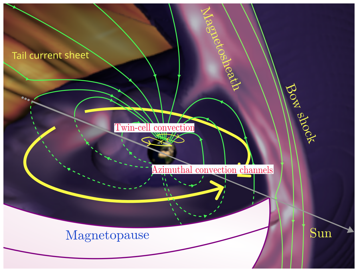
Figure 1 A 3D schematic representation of the Vlasiator simulation run, illustrating both the dayside and nightside magnetosphere. The green lines represent magnetic field lines, while the yellow arrows indicate azimuthal convection channels in the magnetosphere and the twin-cell convection pattern in the ionosphere.

The simulation studied in this paper starts with a non-tilted dipole magnetic field centered at the origin of the simulation box, all defined in the GSM coordinate system. The solar wind is introduced from the positive x boundary, streaming toward the negative x-direction. The box has three dimensions of $x\in [-\mathrm{110}{R}_E,\mathrm{50}{R}_E];y,z\in [-\mathrm{57}{R}_E,\mathrm{57}{R}_E]$. The inner boundary of the simulation is a sphere of 4.7 R_E radius centered on the origin, the magnetosphere is coupling with the ionosphere using a height integrated electrostatic approach (Ganse et al., 2025). Figure 1 depicts the convection and magnetospheric structures during the simulation. In the simulation, a Cartesian grid of cubic cells is utilized, enhanced by static mesh refinement. This refinement achieves the highest spatial resolution 1000 km in regions of interest, such as the bow shock and reconnection sites (Ganse et al., 2023). To further optimize memory and computational efficiency, the simulation employs a sparse velocity space strategy (von Alfthan et al., 2014). In this approach, the velocity distribution is evolved in each spatial cell only when the distribution function f surpasses a specific density threshold f_min (Palmroth et al., 2018). In this specific run, the solar wind parameters are set similarly to those in Horaites et al. (2023), representing fast solar wind conditions: a proton density of 10⁶ m⁻³, a proton temperature of 0.5×10⁶ K, a solar wind velocity of $(-\mathrm{750},\mathrm{0},\mathrm{0})\mathrm{km}{\mathrm{s}}^{-\mathrm{1}}$, and an homogeneous Interplanetary Magnetic Field (IMF) oriented at $(\mathrm{0},\mathrm{0},-\mathrm{5})\mathrm{nT}$.

In this study, we developed a method for estimating the global reconnection voltage based on the instantaneous detection of the closed magnetic flux. The magnetic flux transport is determined by the electric potential on the boundary of a given area by Faraday's law with Stokes' theorem:

$$\begin{array}{}\text{(3)}& \int -{\displaystyle \frac{\partial B}{\partial t}}\cdot \mathrm{d}a=\int \mathrm{\nabla }\times E\cdot \mathrm{d}a=\oint E\cdot \mathrm{d}l.\end{array}$$

The analysis is conducted over a closed contour within the closed field line region. As described by Eq. (3), the rate of change of magnetic flux is determined by the line integral of the electric field E along this contour. Since Eq. (3) applies to a closed contour surrounding a surface rather than an isolated boundary, the contribution to the flux change over each segment of the boundary can be separately evaluated by integrating the electric field along that segment. Specifically, we compute the magnetic flux change rate on the equatorial plane, subdividing the MLTs into 3 h sectors, using spherical coordinates. Convection can be separated into azimuthal (in the θ direction) and radial (in the r direction) components, represented by the electric potentials E_rdr and rE_θdθ, respectively. This approach can be used to calculate the reconnection voltage, which is defined as the rate at which magnetic flux changes topology per unit time, sharing the same dimension as the convection rate. In the Earth's equatorial plane, the reconnection voltage can be determined by the rate of change of closed flux in a region, minus the flux transmitted into that region.

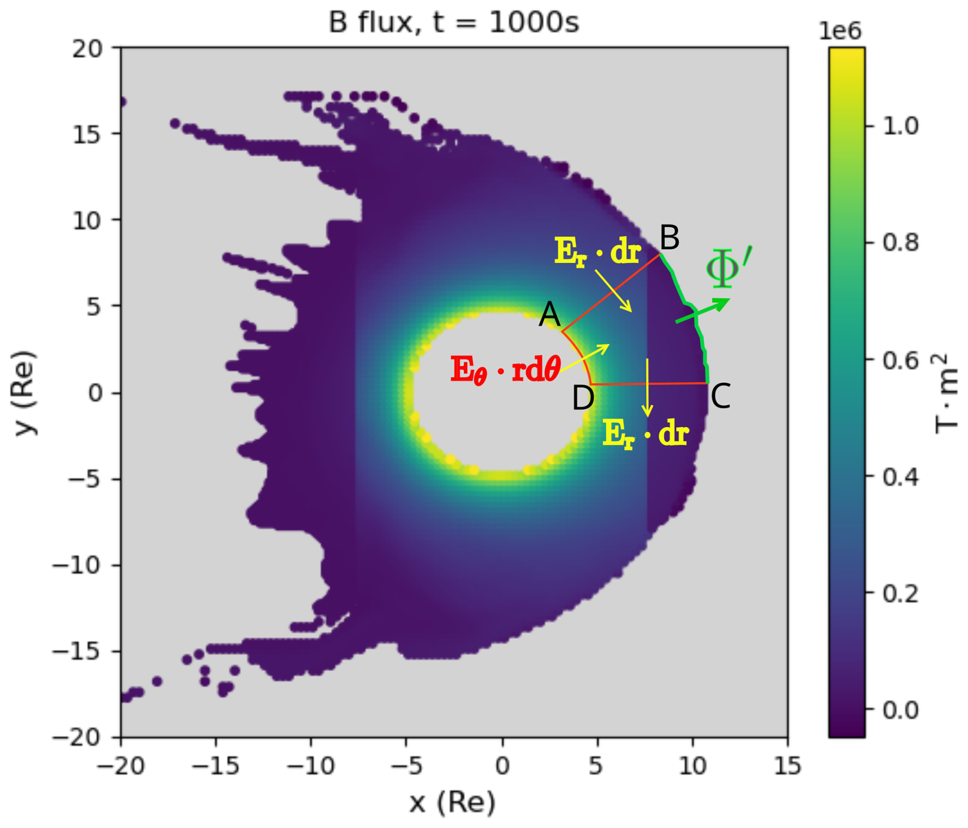
Figure 2 Magnetic flux within the closed field line region in the equatorial plane in the Vlasiator simulation at 1000 s. The grey region represents the area where the magnetic field lines are open. ABCD stands for an enclosed area in the closed field line region on the Earth's equatorial plane. The arrows depict how the magnetic flux flows at the boundaries of the enclosed area.

In Fig. 2, the region ABCD is located within the closed field line area. To determine whether a field line is open or closed in Vlasiator, both ends of the field line are traced to assess whether they connect back to Earth (Pfau-Kempf et al., 2025). In the contour ABCD shown in the figure, AB and CD are sector boundaries. Point B and C both end at OCB. The AD boundary represents the inner edge of Earth’s magnetosphere within the simulation box. The AD and BC boundaries show the radial flow into and out of the sector, while AB and CD represent the azimuthal flow. The radial (r) component of the electric field corresponds to clockwise convection, while the azimuthal (θ) component of the electric field corresponds to outward convection. We equate the reconnection voltage of the sector with the flux transmitted through the boundary BC. The reconnection voltage within an enclosed area ABCD can then be determined by the following equation:

$$\begin{array}{}\text{(4)}& {\mathrm{\Phi }}^{\prime }={\displaystyle \frac{\mathrm{d}{F}_{\mathrm{ABCD}}}{\mathrm{d}t}}-\left(\underset{\mathrm{AB}}{\int }{E}_r\mathrm{d}r-\underset{\mathrm{CD}}{\int }{E}_r\mathrm{d}r+\underset{\mathrm{DA}}{\int }r{E}_{\mathit{\theta }}\mathrm{d}\mathit{\theta }\right).\end{array}$$

Here, $\frac{\mathrm{d}{F}_{\mathrm{ABCD}}}{\mathrm{d}t}$ represents the rate of change of closed flux within the enclosed area, while the other terms on the right side of the equation account for the closed flux entering or leaving through segments AB, AD and CD.

The open magnetic flux content in the polar cap region can be calculated using the following equation (Lockwood, 1993):

$$\begin{array}{}\text{(5)}& F_{\mathrm{PC}}=\underset{\mathrm{PC}}{\int }B\cdot \mathrm{d}s,\end{array}$$

where ds represents the area of open flux, and the integration is performed over the entire polar cap. In the Vlasiator simulation, the process is streamlined by identifying specific markers, or flags, on the ionosphere grid that indicate open magnetic field lines (Horaites et al., 2023).

Next, we aim to find the Dungey cycle convection rate during the simulation, which we defined as the left hand side of Eq. (1) that describes the difference of absolute values between the dayside and nightside reconnection rates. The sum of the reconnection voltages in the four dayside or the four nightside MLT sectors, as given by Eq. (4), represents the dayside or nightside reconnection voltages, respectively. We compare these values with the open flux change rate as given in the right hand side of Eq. (1) to validate the accuracy of the new method.

3 Results

3.1 Dungey Cycle

In this study, we begin by assessing the magnetic flux within the closed field line region, while excluding the region inside the inner boundary of the simulation’s magnetosphere (r=4.7 R_E) as depicted by Fig. 2. Although the field lines inside this inner boundary are closed as well, they are not considered since the propagation solvers are not applied in that region. The convection of the closed magnetic flux within this boundary to the outside is accounted for by an electric field mapped from the ionospheric region of the simulation. In Fig. 3, we divide the Earth’s equatorial plane into eight regions, each corresponding to 3 h of MLT. Our analysis shows that the closed magnetic flux generally increases across most sectors during the simulation, with each sector exhibiting flux on the order of 10⁸ Wb, and the overall flux reaching approximately 10⁹ Wb. This increase is most evident between 800 and 1200 s, particularly in the night sectors, due to the large nightside reconnection voltage shown in Fig. 4. The magnetic flux in the dayside sectors shows a dawn-dusk asymmetry. On the duskside, the magnetic flux enclosed by the MLT 15–18 sector is constantly larger than in the 12–15 sector, while on the dawnside, the two corresponding sectors (6–9 and 9–12 MLT) have approximately the same flux during the simulation. We also observe that the magnetic flux is much lower on the nightside compared to the dayside. Additionally, the magnetic flux in the nightside flank regions (18–21 and 3–6 MLT) is higher than in the central regions (0–3 and 21–0 MLT) in the run.

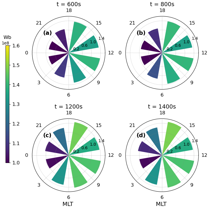
Figure 3 A histogram plot of the magnetic flux (Wb) in the closed field line region of each MLT sectors (3 h interval). Panel (a)–(d) stand for 4 different times in the simulation after the initialization of the simulation. Both the radius and color of each bar represent the magnetic flux in the corresponding MLT sector.

Using Eq. (4), we can now directly calculate the spatiotemporal evolution of magnetic flux in the magnetosphere in our global simulation. Figure 4 presents the reconnection voltages and azimuthal convection rates using a polar plot, similar to Fig. 3. Since reconnection voltages fluctuate significantly on short timescales in the simulation, the data has been smoothed over a 10 s interval. A reflected extension was applied to the first and last time steps to maintain consistency. Colors represent the reconnection voltage in each sector, while arrows indicate convection direction between sectors. The values on the polar plots denote the absolute magnitudes of reconnection and azimuthal convection rates, both in the same units.

Throughout the simulation, azimuthal convection consistently flows from the nightside to the dayside along both the dawn and dusk flanks. The strongest convection is observed at the flanks, specifically at MLT values 15, 18, and 21 on the dusk side, and 3, 6, and 9 on the dawn side. The convection rate remains relatively stable, of the order of 100 kV across these flank sectors. In contrast, the convection rates at the noon (MLT = 12) and midnight (MLT = 0) boundaries are significantly weaker. On average, convection converges near MLT = 12 and diverges near MLT = 0, resulting in net convection rates close to zero. In the simulation, the exact MLT where convergence or divergence are observed can vary, which leads to the fluctuations of azimuthal convection. This behavior is as expected for global convection and aligns with established understanding (Hsieh and Otto, 2014; Dai et al., 2024).

The reconnection voltages exhibit a clear asymmetry between the nightside and dayside. Nightside reconnection is strongest in two MLT sectors (0–3 and 21–0 MLT), as shown in panel (b), although it can also extend into the flank regions. In contrast, dayside reconnection events are more diffusely distributed across all four dayside sectors, indicating a more azimuthally widespread occurrence (Pfau-Kempf et al., 2025). The nightside reconnection voltage is gradually increasing after 600 s, and it peaks at around 800 s. At 600 s, nightside reconnection becomes more intense on the dusk side, which aligns with previous studies showing that the Hall electric field (E_z) generated in the tail strengthens the cross-tail current sheet density in this region (Lin et al., 2014; Lu et al., 2016). By 800 s, reconnection shifts to the dawn sector, where it releases the accumulated magnetic flux. This means that reconnection X-lines develop from dusk to dawn. The dayside remains relatively stable during the simulation. It is worth noting that reconnection voltage in the flank region, especially the nightside flank (18–21 and 3–6 MLT), occasionally exhibits negative values despite the overall positive rates on the nightside. Flux Transfer Events which erode the closed flux on the flank might account for this phenomenon, when they propagate along the magnetopause to the nightside flank regions and transfer the previously closed flux to the solar wind (Pfau-Kempf et al., 2025).

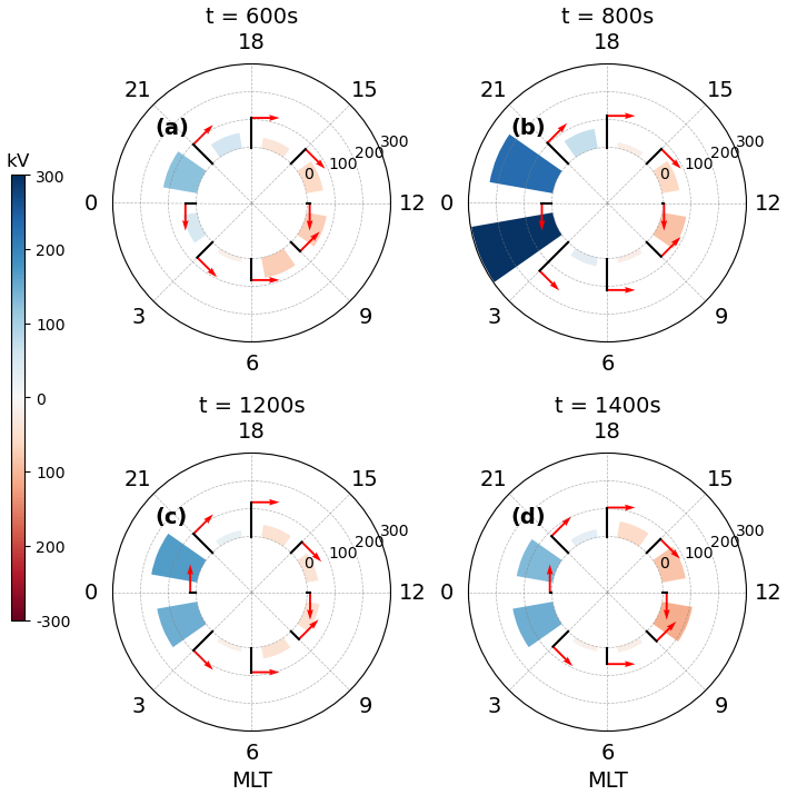
Figure 4 Similar to Fig. 3, but the color scale represents the reconnection voltage. The values here are instantaneous but have been smoothed using a 10 s window. Negative values stand for closed-to-open configuration changes of field lines, while positive values indicate open-to-closed. The red arrows denote the azimuthal convection direction and absolute values of convection rate along the boundaries of MLT sectors.

To validate the Dungey cycle motion and confirm the accuracy of the 3D simulation, it is essential to compare the convection rates within the magnetosphere and ionosphere. In Fig. 5, panel (a) displays the reconnection voltages on the dayside and nightside. These voltages are computed by integrating the reconnection voltages within their respective MLT sectors. Specifically, for the dayside, reconnection voltages are integrated over the 6–18 MLT sector, while for the nightside, the voltages are summed across 18–6 MLT. In panel (b) of Fig. 5, we compare both sides of Eq. (1), where the red points represent the subtraction of absolute values in panel (a) and the dark blue points correspond to the ionospheric magnetic open flux change rate.

The results in panel (a) of Fig. 5 show that the dayside reconnection voltage remains relatively steady at approximately −200 kV throughout the simulation, with some fluctuations. In contrast, the nightside reconnection voltage displays considerable variability. Initially, it is approximately 100 kV at 500 s, rising sharply to nearly 600 kV by 800 s. After reaching this peak, the nightside reconnection voltage gradually decreases, reaching values comparable with the absolute value of the dayside rate at about 1200 s, indicating that the system has entered a quasi-stationary state. Subsequently, the tailward motion of X-lines leads to the stretching of the current sheet and new reconnection bursts, which increases the reconnection voltage at the end of the simulation. Figure 5 panel (b) supports the presence of Dungey cycle motion during the simulation. The total flux transport rate within the closed field line domain, governed by both the dayside and nightside reconnection voltages, should correspond to the open flux change rate in the polar cap. The close alignment between the dark blue and red dots at each time step, despite some fluctuations for the dark blue dots, illustrates this. Panel (b) also demonstrates that the total flux transport rate is near 0 kV at 500 s and decreases to −400 kV at 800 s, gradually returns to 0 kV around 1200 s and then decreases again. This pattern reflects an overall contraction of the polar cap in the simulation from 500 s, with stability occurring when the dayside and nightside reconnection voltages are equal.

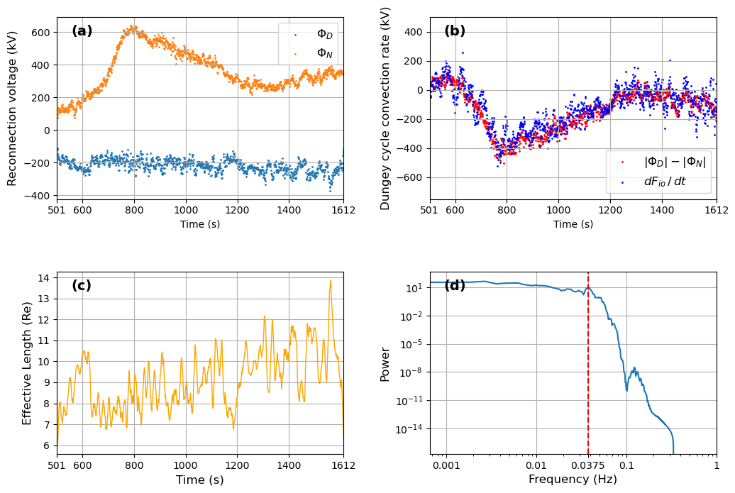
Figure 5 (a) Light Blue dots and orange dots are the dayside and nightside reconnection voltages, respectively. (b) Dungey cycle convection rate obtained with dayside and nightside reconnection voltage (red dots) compared with the open flux change rate (dark blue dots) in the polar cap. The consistency is given by Eq. (1). (c) Dayside reconnection effective length from Eq. (2). (d) Fourier transform of dayside reconnection effective length time series. The red dashed line represents a period of 26.7 s.

Panel (c) of Fig. 5 illustrates the variation in the effective length of the dayside reconnection during the simulation, calculated using Eq. (2). Since the reconnection voltage calculation is based on the equatorial plane, the effective length used is an equivalent length, even though the actual reconnection site may lie outside this plane. The effective length varies between 6 R_E to 14 R_E after 501 s during the simulation, with a mean of 9.12 R_E. A periodic pattern appears to be present in the effective length. As shown in panel (d), the power spectral density, calculated from the Fourier transform of the time series in panel (c), displays a small peak at about 26.7s, suggesting fluctuations in the dayside reconnection effective length at this period. A similar periodicity has been observed in a previous study (Hoilijoki et al., 2019, Fig. 5), which is possibly influenced by mirror mode waves (Hoilijoki et al., 2017). However, the peak is not particularly prominent, and further investigation is required to confirm the presence of this periodicity and its cause.

3.2 Azimuthal Convection

As discussed previously, apart from the magnetic reconnection, the azimuthal convection term also contributes to the magnetic flux change rate in a closed region. The azimuthal convection rate is determined using the second or third term on the right-hand side of Eq. (4). Panel (a) of Fig. 6 shows the azimuthal convection rate plotted against MLT during the simulation. Distinct azimuthal convection channels show up as the darker, oblique stripes, representing periods of elevated convection rates. The average duration of a strong convection channel is about 200 to 300 s, as it travels along the flank of the magnetosphere, from MLT 15 to 21 on the duskside and from MLT 3 to 9 on the dawnside. The convection channels are oriented from noon to midnight over time on both the dawnside and duskside, indicating that these channels originate on the dayside. In panel (b) of Fig. 6, we present the reconnection voltage overlaid with isocontours of the azimuthal convection rate. We observe that the higher dayside reconnection voltages (purple) generally, though somewhat indistinctly, coincide with the bulges of the convection contours. In contrast, despite being generally much stronger, nightside reconnection does not trigger convection channels, as indicated by the nearly vertical convection isocontours in the regions of intense nightside reconnection (dark green). This suggests that the azimuthal convection channels predominantly capture the influence of dayside reconnection, with limited contribution from nightside reconnection. Nevertheless, nightside reconnection can directly induce convection near the midnight sectors, as shown by the dense convection contours near MLT=3 and MLT=21 in panel (b).

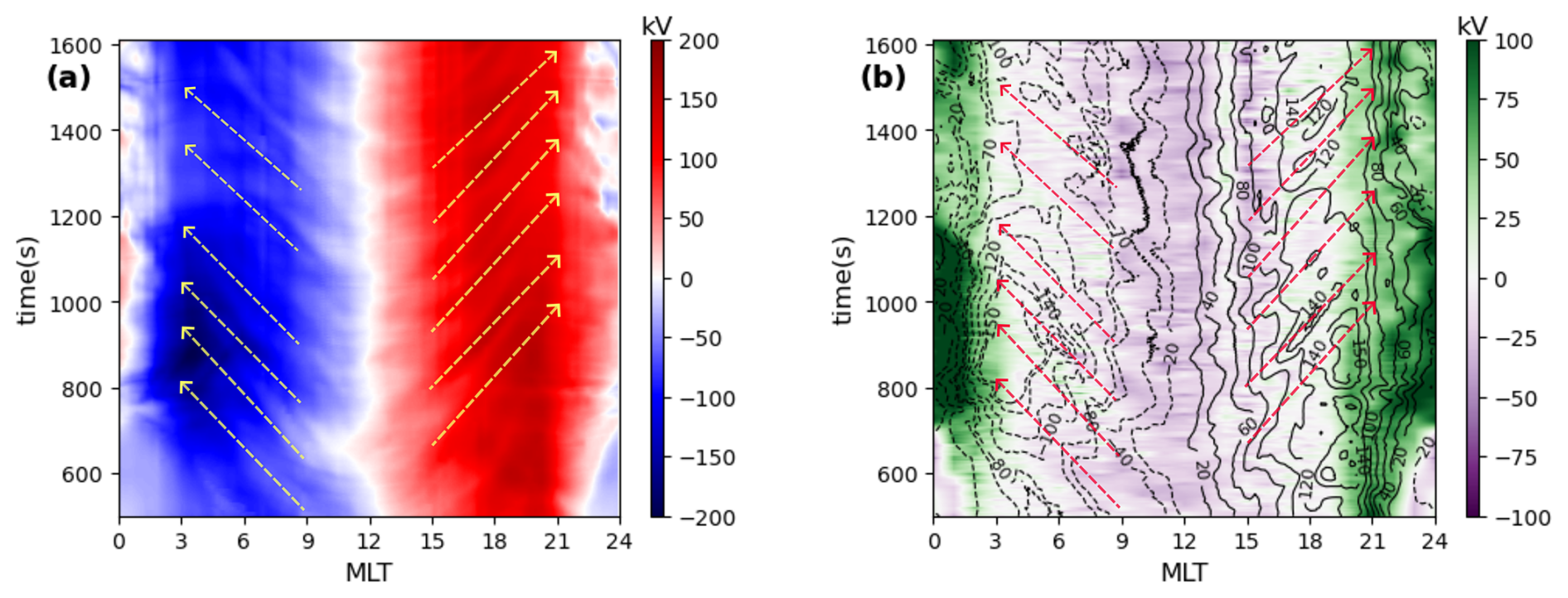
Figure 6 (a) Keogram of azimuthal convection rate on the equatorial plane with time and MLT values. The yellow arrows with dashed lines represent strong convection channels. (b) The color scale represents the reconnection voltage with a 1 h MLT resolution. Isocontours depict the azimuthal convection rate contours from panel (a). The red dashed arrows correspond to the same convection channels as the yellow arrows in panel (a).

In ideal MHD theory, flux tube entropy serves as a key measure of plasma convection. The flux tube entropy parameter is defined as follows (Erickson and Wolf, 1980; Wolf et al., 2009):

$$\begin{array}{}\text{(6)}& S={\left[\int P^{\frac{\mathrm{3}}{\mathrm{5}}}{\displaystyle \frac{\mathrm{d}s}{B}}\right]}^{\frac{\mathrm{5}}{\mathrm{3}}}.\end{array}$$

In this equation, $\frac{\mathrm{d}s}{B}$ represents the volume of a magnetic flux tube per unit magnetic flux and P denotes the plasma pressure. The flux tube entropy parameter can be directly related to the actual entropy in the flux tube (Birn et al., 2009). According to ideal MHD theory, particle motion in the Earth's magnetosphere is isentropic, meaning entropy is conserved along the particle’s path. In other words, plasma is expected to flow along the isocontours of flux tube entropy. However, the hybrid-Vlasov theory diverges from MHD theory by considering the non-Maxwellian distribution functions of ions. As a result, it is important to assess the applicability of ideal MHD theory within the context of our simulation to identify scenarios where the assumptions hold and where they break down.

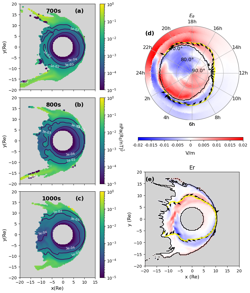
Figure 7 (a)–(c) Flux tube entropy (unit: $\mathrm{nPa}({\mathrm{R}}_{\mathrm{E}}{\mathrm{nT}}^{-\mathrm{1}}{)}^{\frac{\mathrm{5}}{\mathrm{3}}}$) on the equatorial plane at different simulation times, with different values of isocontours. (d) electric field θ component on the ionosphere at 1000 s. (e) electric field r component in the magnetosphere. The yellow contour stands for the entropy isocontour $S=\mathrm{3}\times {\mathrm{10}}^{-\mathrm{3}}\mathrm{nPa}(R_E{\mathrm{nT}}^{-\mathrm{1}}{)}^{\frac{\mathrm{5}}{\mathrm{3}}}$, black contour stands for the OCB, and the black arrows represent the velocity direction along the contour.

In this study, we define pressure using the main diagonal of the thermodynamic pressure tensor from the simulation output, assuming isotropy of pressure consistent with the principles of ideal MHD theory. Figure 7 illustrates flux tube entropy within the closed field line region at three different time steps. Throughout the magnetosphere, flux tube entropy decreases as one moves earthward. This trend aligns with theoretical expectations, as the flux tube volume increases substantially when moving tailward, whereas the pressure exhibits only a slight decrease (Wolf et al., 2009). The order of magnitude of the flux tube entropy varies from ${\mathrm{10}}^{-\mathrm{4}}\mathrm{nPa}(R_E{\mathrm{nT}}^{-\mathrm{1}}{)}^{\frac{\mathrm{5}}{\mathrm{3}}}$ in the inner magnetosphere around 6 R_E to 10⁻¹ at the outer boundary of the magnetosphere. Notably, at each time step illustrated in the panels, regions of lower flux tube entropy are consistently observed near the nightside reconnection sites. These low-entropy regions correspond to phenomena known as Bursty Bulk Flows (BBFs, Sergeev et al., 1996).

Panels (d) and (e) of Fig.  7 show the entropy contour $S=\mathrm{3}\times {\mathrm{10}}^{-\mathrm{3}}\mathrm{nPa}({\mathrm{R}}_{\mathrm{E}}{\mathrm{nT}}^{-\mathrm{1}}{)}^{\frac{\mathrm{5}}{\mathrm{3}}}$ at 1000 s in both the ionosphere and magnetosphere, along with the electric field in θ and r direction respectively. The electric field represents the azimuthal convection rate in both regions. Although the magnitudes differ, the fields in the ionosphere and magnetosphere are closely related. We found that in most regions of the magnetosphere and the ionosphere, the velocity arrows in panel (e) align with the isocontours, indicating an isentropic process. However, the bulk velocity arrows near the reconnection sites and the terminator are not tangent to the contour. This observation contradicts the entropy description of ideal MHD theory.

4 Discussion and conclusion

In this study, we introduced a method for quantifying the magnetic reconnection voltage by examining the flux transport within the closed field line region. The results are validated using the ionospheric proxy given by Eq. (1). We chose this method to estimate the reconnection rate instead of directly calculating it along the X-lines, as the latter approach is particularly challenging. It requires determining the reconnection electric field near the diffusion region, which is difficult to achieve in global simulations due to the presence of multiple X-lines contributing to opening and closing of field lines (Alho et al., 2024). This selected method circumvents the need to identify and attribute to specific X-lines.

One particular event around 11 UT on 26 August 1998, reported by Milan et al. (2007), exhibited solar wind conditions similar to those used in our simulation. During this event, the solar wind B_z component was around −5 nT, and the V_x component was approximately 650 km s⁻¹ directed toward the Earth. Under these conditions, Milan et al. (2007) estimate a dayside reconnection voltage of about 300 kV, which aligns reasonably well with our simulation results.

However, our overall reconnection voltages for both the dayside and nightside are significantly higher than the mean observational data reported by Milan et al. (2007). Their study, based on 25 events, estimated a mean dayside reconnection voltage of 31 kV and a mean nightside reconnection voltage of 85 kV, whereas our simulation yields a mean dayside reconnection voltage of 217 kV and a mean nightside reconnection voltage of 362 kV after 500 s. This discrepancy may be attributed to our simulation setup. We assume a constant southward IMF and a high solar wind velocity, which rapidly transports IMF lines to the dayside throughout the runtime, and leads to a higher energy input. This setup does not account for the highly variable solar wind conditions and substorm dynamics observed in reality. Real-world reconnection events are often modulated by fluctuations in the IMF and solar wind pressure, as well as lower solar wind velocities (Boudouridis et al., 2007; Toledo-Redondo et al., 2021). Observational studies have also shown that dayside reconnection is directly influenced by IMF fluctuations (Dai et al., 2023). These factors contribute to a more variable and generally lower reconnection voltage and energy input. Consequently, the solar wind conditions in our simulation may have led to an overestimation of the reconnection voltage in our model.

Magnetic reconnection during the simulation is consistent with the current understanding of reconnection dynamics, where the midnight sector is recognized as the primary site for current sheet formation, while dayside reconnection is typically driven by interactions with the incoming, shocked solar wind at the magnetopause (Runov et al., 2022; Koga et al., 2019). At 600 s, nightside reconnection intensifies on the dusk side, consistent with prior studies that demonstrate the role of the Hall electric field in this region (Lin et al., 2014; Lu et al., 2016). Specifically, the Hall electric field generated in the tail enhances the cross-tail current sheet density, further reinforcing reconnection activity in the dusk sector. Given the ion-kinetic nature of the simulation, researchers have been focusing on exploring ion-kinetic signatures (Palmroth et al., 2023; Cozzani et al., 2025; Zaitsev et al., 2025). Building on these works, we plan to further investigate features such as Hall electric field and off-diagonal components of the ion pressure tensor in the magnetotail reconnection region.

An alternative method for estimating the reconnection voltage in the ionosphere relies on calculating the electric field along the polar cap boundary, along with the velocity of the ionospheric convection and OCB, primarily based on observational data (de La Beaujardiere et al., 1991; Blanchard et al., 1997; Hubert et al., 2006; Gasparini et al., 2024). However, we did not employ this approach for several reasons. First, our method of computing reconnection voltage across different MLT sectors inherently yields the azimuthal convection rate as a by-product, which is an important quantity for our analysis. Secondly, while this alternative method may allow validation of the obtained reconnection voltage via an independent method, determining the velocity of the OCB is difficult in the simulation because of the limited refinement level and highly dynamic nature near the reconnection sites. According to Blanchard et al. (1997); Gasparini et al. (2024), typical OCB velocities are on the order of a few hundred meters per second. Since the finest spatial resolution of the ionosphere is 62km in our simulation (Ganse et al., 2025) in order to match Vlasov domain cell size at the inner boundary, the typical velocities of the OCB remain unresolvable. In addition, simply increasing the ionospheric grid resolution alone would not improve the accuracy meaningfully, as it would introduce additional computational cost and amplify Vlasov grid artifacts in the ionosphere mappings. Therefore, resolving the OCB motion remains beyond the capabilities of the current model configuration. Third, one of the objectives of this work is to assess the coupling between the inner boundary and the ionosphere in the simulation, and thus relying on ionospheric parameters will compromise this goal.

The azimuthal convection channels in our simulation exhibit non-continuous behavior despite the constant solar wind input. Distinct convection channels are clearly initiated at the dayside magnetopause, propagating to the nightside, and appear to be driven by dayside reconnection events. However, the duration of the convection channels, approximately 200–300 s in the dawn and dusk sectors, is shorter than estimates from previous MHD simulations, such as those reported by Dai et al. (2024). Their study, based on OMNI data from 11 March 2016, featured a lower velocity in the solar wind V_x component and a varying IMF. The solar wind conditions in the simulation could be a reason that influence the duration of the azimuthal convection channels.

In addition, we observed that the ideal MHD assumption, which posits that plasma flow follows the isocontours of flux tube entropy, holds true only in certain regions of the Earth's magnetosphere. In the vicinity of reconnection sites and the terminators, plasma convection deviates from isentropic behavior, indicating the presence of non-adiabatic processes in these regions. This finding suggests that the assumption of ideal MHD of plasma particle trajectories (Wolf et al., 2009, Fig. 1) breaks down in those areas, where the plasma's kinetic and thermal energy are redistributed in ways that violate isentropic conditions. The deviation near reconnection sites is expected, as reconnection inherently involves non-Maxwellian ion distributions and Hall effect, which are not captured in ideal MHD models. Those processes contribute to the violation of isentropic conditions. However, the deviation observed where the terminator intersects the entropy isocontour at panel (e) of Fig. 7 is more surprising, as the ideal MHD assumption should hold in this region. The terminator region shown in that panel is far from reconnection sites and particle motions in these areas should be explained by ideal MHD theory. This unexpected behavior warrants further investigation to better understand the underlying processes.

In this study, we investigated magnetospheric convection using a hybrid-Vlasov simulation. We proposed a new method for quantifying the Dungey Cycle convection throughout the simulation, revealing convection rate variations ranging from −400 to 200kV. The proposed method is validated by comparing the results with ionospheric open flux change rate. Our findings show that the nightside reconnection initiates on the dusk side, and the dayside reconnection voltage exhibits a periodicity of 26.7s. The dayside reconnection effective length varies between 6 to 14 R_E, which is comparable to previous studies (Milan et al., 2007). In addition, we identified discrete azimuthal convection channels that are associated with dayside reconnection events. Finally, we observed that plasma convection within the closed field line regions is not strictly aligned with isentropic contours near reconnection cites and twilight zones. This suggests that plasma convection within the magnetosphere cannot be fully described by ideal MHD theory.