Indications for particle precipitation impact on the ion-neutral collision frequency analyzed with EISCAT measurements

The ion-neutral collision frequency is a key parameter for the coupling of the neutral atmosphere and the ionosphere. Especially in the mesosphere lower–thermosphere (MLT), the collision frequency is crucial for multiple processes, e.g., Joule heating, neutral dynamo effects, and momentum transfer due to ion drag. Few approaches exist to directly infer ion-neutral collision frequency measurements in that altitude range. We apply the recently demonstrated difference spectrum fitting method to obtain the ion-neutral collision frequency from dual-frequency measurements with the EISCAT incoherent scatter radars in Tromsø. A 60 h long EISCAT campaign was conducted in December 2022. Strong variations of nighttime ionization rates were observed with electron densities at 95 km altitude varying from $N_{\mathrm{e},\mathrm{95}}\sim {\mathrm{10}}^{\mathrm{9}}$ to 10¹¹ m⁻³, which indicates varying levels of particle precipitation. A second EISCAT campaign was conducted on 16 May 2024, capturing a solar energetic particle (SEP) event, exhibiting constantly increased ionization due to particle precipitation in the lower E region: $N_{\mathrm{e},\mathrm{95}}\gtrsim \mathrm{5}\times {\mathrm{10}}^{\mathrm{10}}{\text{m}}^{-\mathrm{3}}$. We demonstrate variations of the ion-neutral collision frequency profile that we interpret as neutral particle uplift due to particle precipitation heating. Assuming a rigid-sphere particle model, we derive neutral density profiles which indicate a significant variation of neutral gas density between about 90–110 km altitude that correlate with the estimated strength of particle precipitation. However, the change in ion-neutral collision frequencies cannot be conclusively linked to the particle precipitation impact, and alternative interpretations are discussed. We additionally test the sensitivity of the difference spectrum method to various a priori collision frequency profiles.

1 Introduction

The neutral atmosphere dynamics in the mesosphere lower–thermosphere (MLT) region are affected by the lower-atmospheric wave-driven dynamics and the forcing due to space weather (Liu, 2016). Therefore, this region is significant for atmosphere–ionosphere coupling and consequently the impact of space weather on the Earth system including the middle and lower atmosphere. Although the neutral particle density in the MLT region can only be measured in situ, it still is possible to infer the ion-neutral collision frequency ν_in from remote sensing measurements. The ion-neutral collision frequency is directly correlated with the particle density of the neutral atmosphere n_n. Assuming rigid-sphere collisions, the ion-neutral collision frequency is given by Chapman (1956):

$$\begin{array}{}\text{(1)}& {\mathit{\nu }}_{\mathrm{in}}=\mathrm{2.6}\times {\mathrm{10}}^{-\mathrm{9}}\cdot \left(n_{\mathrm{n}}\left[{\text{cm}}^{-\mathrm{3}}\right]+n_{\mathrm{i}}\left[{\text{cm}}^{-\mathrm{3}}\right]\right)\cdot A^{-\mathrm{0.5}}.\end{array}$$

Here, the mean molecular ion mass A is given in atomic mass units. Equation (1) assumes that the density of the neutral atmosphere is significantly larger than the ion density n_i (which is assumed to be equal to the electron density n_e). There are several alternative ways to describe ion-neutral collisions, e.g., Maxwell collisions of ions and polarized neutrals (Schunk and Walker, 1971). Additionally, resonant collisions of neutrals with their first positive ion (e.g., O₂ and O${}_{\mathrm{2}}^{+}$) strongly increase the total collision frequency above certain temperature thresholds (Ieda, 2020). In this paper, Eq. (1) is applied to relate the ion-neutral collision frequency, and the neutral density and potential deviations are discussed in Sect. 5.

ν_in is known to impact the shape of a spectrum for incoherent scatter radar (ISR) measurements (Grassmann, 1993a; Akbari et al., 2017). Previous studies have demonstrated that the ion-neutral collision frequency can be obtained from dual-frequency ISR measurements (Grassmann, 1993b; Nicolls et al., 2014; Günzkofer et al., 2023b). However, dual-frequency ISR measurements are, at the moment, only possible with the EISCAT ultrahigh- and very-high-frequency (UHF and VHF) radars. Therefore, the total number of dual-frequency ISR measurements remains sparse. Additionally, the multi-parameter analysis for two ISR spectra as proposed by Nicolls et al. (2014) is not part of the standard ISR analysis software. The difference spectrum fitting described in Grassmann (1993b) and demonstrated by Günzkofer et al. (2023b) overcomes this problem by combining the two spectra after the standard single-frequency analysis. Although the difference spectrum method has been known for several decades, a systematic application of the technique is still missing, and thus the ion-neutral collision frequency and neutral density in the MLT region have not been studied extensively by leveraging dual-frequency EISCAT observations.

One forcing mechanism specifically important at high latitudes is the precipitation of energetic particles along the magnetic field lines down to MLT altitudes. These particles contribute significantly to the ionization and the heating of the high-latitude thermosphere. In the MLT region, mainly precipitating electrons with energies of 10–100 keV and protons with energies of about 1 MeV contribute to the ionization of the atmosphere (Fang et al., 2010, 2013). Additionally, it has been shown that the heating due to the absorption of (extreme) ultraviolet radiation and Joule heating alone is not sufficient to explain the observed thermosphere dynamics (Smith et al., 1982). Thermospheric heating leads to an upwelling of the neutral atmosphere and therefore causes distinct increases in the neutral particle density and consequently also the ion-neutral collision frequency ν_in at certain altitudes (Hays et al., 1973; Olson and Moe, 1974; Kurihara et al., 2009; Oyama et al., 2012). The additional ionization due to particle precipitation also increases the ionospheric conductivity and thereby the Joule heating (Vickrey et al., 1982). Both the direct particle precipitation heating and the additional Joule heating contribute significantly to the generation of ionospheric irregularities, e.g., large-scale traveling ionospheric disturbances (Sheng et al., 2020; Nykiel et al., 2024). It can be seen that the particle precipitation in the MLT region plays a crucial role in space weather research and the development of thermosphere–ionosphere models (Zhang et al., 2019; Watson et al., 2021).

In this study, we investigate the impact of particle precipitation on the vertical profiles of ion-neutral collision frequency and neutral particle density in the MLT region. The ion-neutral collision frequency is inferred from combined EISCAT UHF and VHF measurements. The particle precipitation impact can be estimated from EISCAT electron density measurements. The measurement campaigns with the EISCAT ISRs are described in Sect. 2. The difference spectrum method applied to determine ion-neutral collision frequencies and the estimation of the particle precipitation energy impact is described in Sect. 3. The obtained results are presented in Sect. 4. In Sect. 5, how other processes like atmospheric tides and Joule heating might contribute to the observed variation of the ion-neutral collision frequency is discussed. Additionally, the low electron densities in the MLT region lead to considerable uncertainties in ISR measurements. The potential issues of increased data noise for the difference spectrum method are discussed in Sect. 5. The paper is concluded in Sect. 6 including an outlook on potential future work.

2 EISCAT UHF and VHF measurements

Dual-frequency ISR measurements can be performed with the ultrahigh-frequency (UHF) and very-high-frequency (VHF) radars near Tromsø, Norway (69.6° N, 19.2° E), operated by the EISCAT Scientific Association (Folkestad et al., 1983). The UHF ISR applies a radar frequency of 929 MHz with a nominal power of about 1.5–2 MW, and the VHF ISR transmits at a radar frequency of 224 MHz and has a nominal power of about 1.5 MW. The dual-frequency analysis requires both systems to be operated in the same radar mode and beam pointing to ensure overlapping observation volumes. A summary of all EISCAT instruments and experimental modes can be found in Tjulin (2024).

In this study, we leverage a 60 h long dual-frequency EISCAT campaign conducted from 13 December 2022 at 00:00 UT to 15 December 2022 at 12:00 UT during the Geminids meteor shower. A second EISCAT campaign, conducted on 16 May 2024 at 06:00–15:00 UT, is analyzed as well. This campaign was scheduled to be conducted during a solar energetic particle (SEP) event and therefore exhibits high particle precipitation rates. The strength of the auroral electrojet during both measurement campaigns is estimated from the SuperMAG SME index (Newell and Gjerloev, 2011; Gjerloev, 2012) shown in Fig. 1.

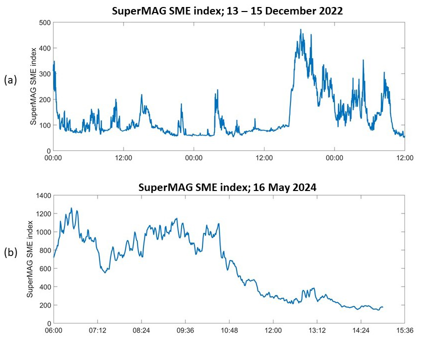
Figure 1 SuperMAG auroral electrojet index SME during the EISCAT campaigns in (a) December 2022 and (b) May 2024.

During both campaigns, the UHF and VHF radars were pointed in the zenith using the manda pulse code, which is optimized for high-resolution D-region measurements (as used in the EISCAT Common Programme 6). By default, manda measurements are analyzed in very narrow range gates with an altitude resolution of a few hundred meters up to 110 km altitude. However, for small electron densities, this results in very noisy data, which causes problems with both the standard plasma parameter analysis and the dual-frequency analysis of collision frequencies. Therefore, we adjusted the altitude gates to 250 logarithmically spaced gates from 50–200 km altitude. In the MLT region, this results in an altitude resolution of approximately 3 km. For the same reason, the commonly applied integration window length of 60 s was extended to 120 s. The potential issues arising with altitude gates that are too narrow and integration windows that are too short are discussed in Sect. 5. The standard analysis software for EISCAT ISR measurements is the Grand Unified Incoherent Scatter Design and Analysis Package (GUISDAP) (Lehtinen and Huuskonen, 1996). For the analysis presented in this paper, the GUISDAP Version 9.2 was applied.

3 Methods

3.1 Difference spectrum fitting

Difference spectrum fitting is one of three methods to obtain ion-neutral collision frequencies from dual-frequency ISR measurements proposed by Grassmann (1993b). It was applied in Günzkofer et al. (2023b), where a detailed description of the method is given. The main advantage of the difference spectrum fitting is that it is based on the standard EISCAT ISR analysis package GUISDAP. Therefore, the implementation of specific software for the joint analysis of two ISR measurements as described in Nicolls et al. (2014) is not required.

In the first step, the UHF and VHF measurements are analyzed separately, and in the second step, the obtained ISR spectra are combined. In this second step, the measured VHF spectrum is scaled to UHF frequencies with the UHF-to-VHF frequency ratio ξ≈4.15. The scaled VHF spectrum is equivalent to a UHF spectrum for an electron density ξ²⋅n_e and an ion-neutral collision frequency ξ⋅ν_in. Hence, the collision frequency ν_in is inferred from the difference between UHF and scaled VHF spectra. Technical differences between the two radars are accounted for by introducing the so-called β parameter, which is determined from the measurements at the uppermost range gate corresponding to approximately 200 km altitude. At this height, we assume a collisionless ionosphere, i.e., ν_in≪ω_i with the ion gyrofrequency ω_i, and thus the remaining differences are most likely given by system-specific factors such as beam width and differences in the observation volume. A detailed description of this procedure and the impact of varying β parameters is outlined in Günzkofer et al. (2023b), Sects. 3 and 4.

3.2 Particle precipitation estimate

Precipitating particles affect the MLT by ionizing the neutral molecules in that region. The ionization electrons are thermalized and thereby heat both the ionosphere plasma and the MLT neutral atmosphere. Assuming particle precipitation to be the dominant ionization process, the energy deposition can be estimated from ISR electron density measurements. Vickrey et al. (1982) demonstrated a method to determine the particle precipitation energy deposition assuming an empirical profile for the effective recombination coefficient. However, it has been shown that the effective recombination coefficient profile depends on the precipitating particles (electrons or protons) and energy (Gledhill, 1986). As an approximate quantification for the total particle precipitation impact, the electron density at 95 km altitude N_e,95 measured with the EISCAT VHF ISR is applied. The validity of this approximation and possible problems are discussed in Sect. 5.

4 Results

4.1 EISCAT Geminids campaign, December 2022

As described in Sect. 2, a 60 h dual-frequency EISCAT campaign from December 2022 is analyzed. Figure 2 shows the measured electron density and the ion-neutral collision frequency calculated with the difference spectrum method. Both quantities are shown at 85–110 km altitude where we expect particle precipitation to have the strongest impact. At higher altitudes, the Joule heating would become more and more significant (see Sect. 5) (Baloukidis et al., 2023; Günzkofer et al., 2024). The electron density at 95 km altitude N_e,95 that is applied as a quantification for the particle precipitation impact is shown as well. Since the manda experiment mode is optimized for the EISCAT VHF radar, the electron density is taken from these measurements. The time axis in Fig. 2 is given in Universal Time (UT). The local apparent solar time (LAST) at Tromsø (∼20° E) is approximately UT+80 min.

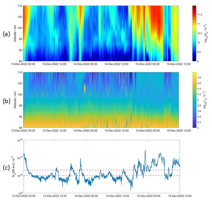
Figure 2 EISCAT measurements from 13 December 2022 at 00:00 UT to 15 December 2022 at 12:00 UT. (a) EISCAT VHF electron density, (b) ion-neutral collision frequency from combined VHF and UHF measurements, and (c) N_e,95 from the VHF electron density.

It can be seen in Fig. 2a that the electron density is significantly increased at nighttime. At high latitudes, it can be assumed that particle precipitation is the dominant source of nighttime ionization. During the last night from 14 to 15 December, the increase in electron density is much stronger than in the two nights before, indicating strong particle precipitation presumably due to substorm activity (see Fig. 1). The electron density at 95 km altitude in Fig. 2c shows maxima on 13 December at about 00:40 and 22:00 UT, as well as from 14 December at 19:00 UT to 15 December at 04:00 UT. At the times of high N_e,95, Fig. 2b shows that the ion-neutral collision frequency is strongly increased at altitudes ≳95 km. This suggests an effect of particle precipitation on the ion-neutral collision frequency.

To investigate the daily mean variation of the ion-neutral collision frequency, we bin the measured profiles into four LAST sectors (midnight, dawn, noon, and dusk). Figure 3 shows the median profiles for the four bins and two climatology profiles. The first climatology profile is applied as the a priori profile for the EISCAT ISR analysis. In this case, the a priori climatology is taken from the CIRA2014 neutral atmosphere model (Rees et al., 2013). The applied climatology model, however, depends on the GUISDAP version and installation. The second climatology profile is calculated from the empirical NRLMSIS 2.0 model for neutral densities (Emmert et al., 2021). As already seen in Günzkofer et al. (2023b), the two climatologies are different by a factor of ∼1.5–2, but both show a smooth exponential decrease in the collision frequency with increasing altitude. So in addition to the LAST binning, Fig. 3 shows ion-neutral collision frequency profiles derived from EISCAT by initializing the difference spectrum fit with (a) the EISCAT a priori and (b) the NRLMSIS climatological profile, respectively.

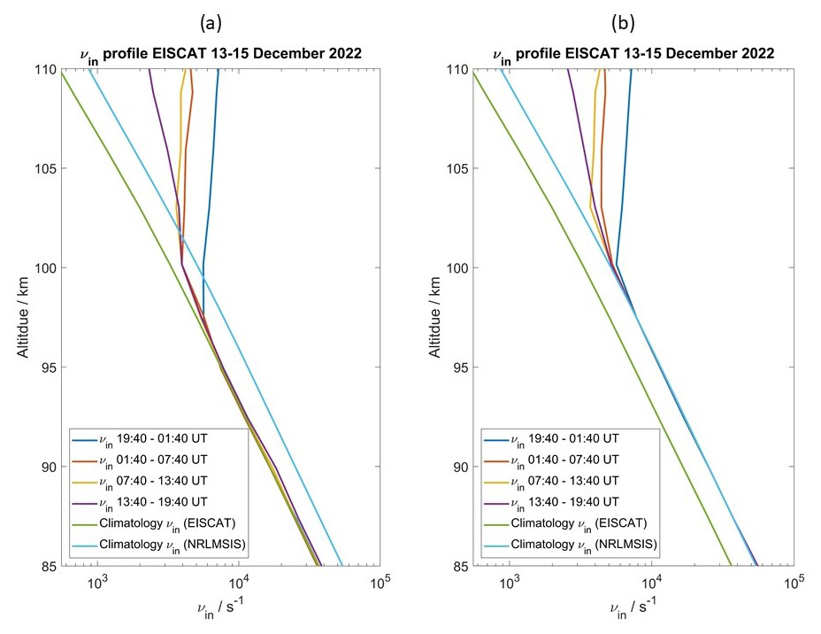
Figure 3 Median vertical profiles of the ion-neutral collision frequency for local apparent solar midnight, dawn, noon, and dusk sectors compared to climatology profiles. As the a priori profile for the difference spectrum fit, (a) the EISCAT single-frequency ν_in or (b) ν_in calculated from NRLMSIS results can be applied. The impact of the a priori on the difference spectrum fit is discussed in Sect. 5 and illustrated in Fig. 9.

Below 100 km altitude the difference spectrum ν_in profile appears to be strongly affected by the choice of a priori profile. However, it can be seen in Fig. 3a that above 95 km, the difference spectrum fit starts to deviate from the EISCAT a priori profile towards the NRLMSIS profile. This agrees well with the results found in Günzkofer et al. (2023b). In Sect. 5, at which altitude the difference spectrum fit is a priori dominated is discussed.

Above 100–105 km and with increasing electron density, our fitting approach starts to get more and more independent of the choice of the a priori profile, which is indicative of a sufficient measurement response. At the highest investigated altitude of 110 km, the four profiles give very similar values in both plots. Also, the daily variation of ν_in above 100 km altitude is identical in Fig. 3a and b. It can be seen that the ion-neutral collision frequency is significantly increased during the LAST midnight and dawn sectors. The lowest ν_in values are found during the LAST noon and dusk sectors.

The diurnal variation found in Fig. 3 fits the impact of particle precipitation, especially the dawn–dusk asymmetry as the particle precipitation energy deposition is known to be larger around the morning hours (Vickrey et al., 1982). In the next step, we separate the vertical profiles of the ion-neutral collision frequency ν_in with respect to the particle precipitation impact, quantified by N_e,95. We define three ranges for low, medium, and high particle precipitation at $N_{\mathrm{e},\mathrm{95}}<\mathrm{1}\times {\mathrm{10}}^{\mathrm{10}}{\text{m}}^{-\mathrm{3}}$, $\mathrm{1}\times {\mathrm{10}}^{\mathrm{10}}{\text{m}}^{-\mathrm{3}}<N_{\mathrm{e},\mathrm{95}}<\mathrm{2}\times {\mathrm{10}}^{\mathrm{10}}{\text{m}}^{-\mathrm{3}}$, and $N_{\mathrm{e},\mathrm{95}}>\mathrm{2}\times {\mathrm{10}}^{\mathrm{10}}{\text{m}}^{-\mathrm{3}}$. For each bin, the median vertical ν_in profile is calculated. For this analysis, we only apply the collision frequencies obtained from the dual-frequency fit initialized with the NRLMSIS climatology.

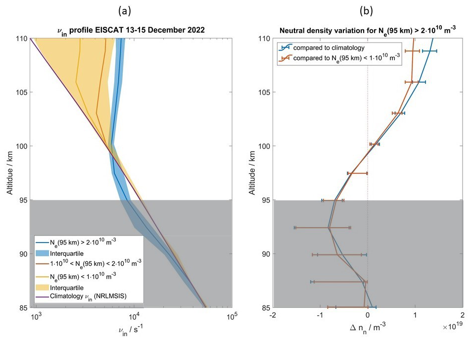
Figure 4 (a) Median vertical collision frequency profiles binned with N_e,95. (b) Difference in neutral particle densities calculated from the collision frequency profiles for high and low particle precipitation. The gray-shaded areas indicate the altitudes at which the difference spectrum fit is a priori dominated (see Sect. 5).

Figure 4a shows the median profiles for the three bins and the climatology profile. The interquartile range is shown for the bins with lowest and highest N_e,95 profiles, indicating the volatility of the difference spectrum fit for low electron densities. Dual-frequency ν_in measurements are highly unreliable for low ionization conditions. However, it still appears to be evident that ν_in increases with increasing particle precipitation energy deposition above about 100 km altitude, which explains the daily variation found in Fig. 3. Additionally, we found a characteristic decrease in the ion-neutral collision frequency for high N_e,95 at altitudes of about 90–100 km. It can be seen that for higher particle precipitation impact, the ν_in profiles deviate from the a priori profile at lower altitudes. For the lowest particle precipitation impact ($N_{\mathrm{e},\mathrm{95}}<\mathrm{1}\times {\mathrm{10}}^{\mathrm{10}}{\text{m}}^{-\mathrm{3}}$), the collision frequency fit is dominated by the a priori profile up to 100 km altitude and mostly unreliable at higher altitudes. The statistical interquartile uncertainties of the high-particle-precipitation profile are shown as a blue-shaded area in Fig. 4a. The gray-shaded areas indicate the altitudes at which the difference spectrum fit is a priori dominated and the results cannot be considered reliable (see Sect. 5).

The decrease in ν_in at ∼90–100 km and increase in ν_in at ≳100 km altitude with larger N_e,95 indicates uplift of neutral particles. Applying Eq. (1), we can calculate the vertical profile of neutral particle density n_n from the collision frequency profiles. Figure 4b shows the difference of the n_n profiles obtained from the ν_in profiles for $N_{\mathrm{e},\mathrm{95}}>\mathrm{2}\times {\mathrm{10}}^{\mathrm{10}}{\text{m}}^{-\mathrm{3}}$ compared to the low-particle-precipitation profile ($N_{\mathrm{e},\mathrm{95}}<\mathrm{1}\times {\mathrm{10}}^{\mathrm{10}}{\text{m}}^{-\mathrm{3}}$) and the climatology profile. The depletion of the neutral particle density below 100 km is approximately equal to the increase above 100 km. In absolute numbers, the maximum n_n decrease or increase is $\pm {\mathrm{10}}^{\mathrm{19}}{\text{m}}^{-\mathrm{3}}$.

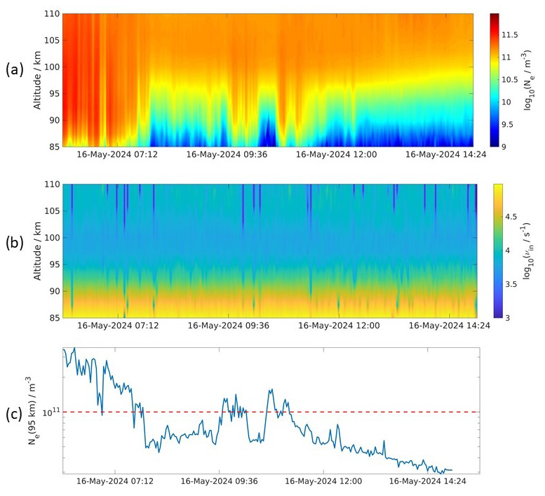
Figure 5 (a) EISCAT VHF electron density, (b) ion-neutral collision frequency from combined VHF and UHF measurements, and (c) electron density at 95 km altitude from the VHF measurements.

4.2 EISCAT SEP campaign, May 2024

The dual-frequency EISCAT campaign conducted on 16 May 2024 was scheduled to be triggered by an SEP event. This allows us to study the impact of continuously high particle precipitation rates on the ion-neutral collision frequency over several hours. At approximately 100 km altitude, the main impact of particle precipitation is caused by auroral electrons (Mironova et al., 2015). We focused our analysis on the campaign period with EISCAT measurements on 16 May 2024 from 06:00–15:00 UT. Figure 5 shows (a) the electron density, (b) the ion-neutral collision frequency, and (c) N_e,95 on 16 May 2024.

The major difference compared to the first campaign is that the electron density in Fig. 5a is generally larger than in Fig. 2a. This is presumably caused by the increased particle precipitation energy deposition and consequently increased ionization rate due to the SEP event. The increased electron density improves the signal-to-noise ratio (SNR) for all altitudes above 95 km. Since the solar zenith angle at the Tromsø geographic latitude is significantly lower in May compared to December, photoionization presumably contributes to the E-region ionization. This is discussed in Sect. 5.

EISCAT measurements indicate $N_{\mathrm{e},\mathrm{95}}>\mathrm{2}\times {\mathrm{10}}^{\mathrm{10}}{\text{m}}^{-\mathrm{3}}$ for the entire campaign period on 16 May 2024. Therefore, all measurements on 16 May 2024 would fall in the highest N_e,95 range by which ν_in was sorted in Fig. 4a. The ion-neutral collision frequency measurements are binned with the electron density at 95 km altitude. Two bins are applied for N_e,95 values larger or smaller than $\mathrm{1}\times {\mathrm{10}}^{\mathrm{11}}{\text{m}}^{-\mathrm{3}}$. Figure 6a shows the two ν_in profiles from 16 May 2024 in comparison to the NRLMSIS climatology profile and the $N_{\mathrm{e},\mathrm{95}}>\mathrm{2}\times {\mathrm{10}}^{\mathrm{10}}{\text{m}}^{-\mathrm{3}}$ profile from December 2022.

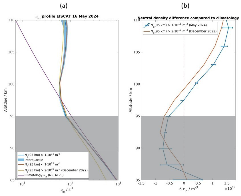
Figure 6 (a) Median ion-neutral collision frequency profiles from 16 May 2024 binned for N_e,95 values larger or smaller than $\mathrm{1}\cdot \mathrm{1}{\mathit{ß}}^{\mathrm{11}}{\text{m}}^{-\mathrm{3}}$. The ν_in profile from December 2022 for $N_{\mathrm{e},\mathrm{95}}>\mathrm{2}\times {\mathrm{10}}^{\mathrm{10}}{\text{m}}^{-\mathrm{3}}$ is shown for comparison. (b) Difference of the neutral density profiles calculated for $N_{\mathrm{e},\mathrm{95}}>\mathrm{1}\times {\mathrm{10}}^{\mathrm{11}}{\text{m}}^{-\mathrm{3}}$ and $N_{\mathrm{e},\mathrm{95}}>\mathrm{2}\times {\mathrm{10}}^{\mathrm{10}}{\text{m}}^{-\mathrm{3}}$ (December 2022) in comparison to the respective climatology profiles for May and December. The gray-shaded areas indicate the altitudes at which the difference spectrum fit is a priori dominated (see Sect. 5).

For the May campaign we found that the two ν_in profiles for $N_{\mathrm{e},\mathrm{95}}>\mathrm{1}\times {\mathrm{10}}^{\mathrm{11}}{\text{m}}^{-\mathrm{3}}$ and $N_{\mathrm{e},\mathrm{95}}<\mathrm{1}\times {\mathrm{10}}^{\mathrm{11}}{\text{m}}^{-\mathrm{3}}$ are nearly identical and highly similar to the $N_{\mathrm{e},\mathrm{95}}>\mathrm{2}\times {\mathrm{10}}^{\mathrm{10}}{\text{m}}^{-\mathrm{3}}$ profile from December 2022. Below about 90 km altitude, the seasonal variation of the NRLMSIS climatology that is used to initiate the dual-frequency ν_in fit causes the profiles to deviate. However, there are additional differences between the December 2022 and May 2024 profiles above 90 km altitude, presumably caused by the difference in the strength of particle precipitation. Equation (1) is applied to calculate the neutral particle density n_n profiles from the $N_{\mathrm{e},\mathrm{95}}>\mathrm{1}\times {\mathrm{10}}^{\mathrm{11}}{\text{m}}^{-\mathrm{3}}$ collision frequency profile. The difference in neutral particle density Δn_n between the $N_{\mathrm{e},\mathrm{95}}>\mathrm{1}\times {\mathrm{10}}^{\mathrm{11}}{\text{m}}^{-\mathrm{3}}$ and climatology profile is calculated equivalent to the blue Δn_n profile in Fig. 4b. Both Δn_n profiles are shown in Fig. 6b.

It can be seen that the Δn_n profile for May 2024 is shifted to lower altitudes by about 2 km compared to the December 2022 profile. Assuming particle precipitation to be the cause for the observed changes, this would mean that the deposition altitude is slightly lower during the May 2024 measurements, indicating a higher particle energy. However, the increase or decrease in neutral particles is of similar magnitude at about 10¹⁹ m⁻³.

5 Discussion

The presented work presumably shows the impact of particle precipitation on the ion-neutral collision frequency. However, the presented results have considerable uncertainties regarding both the obtained results themselves and their interpretation. The following issues will be discussed in this section:

• EISCAT data noise for low electron densities in the MLT region,

• the impact of a priori parameter assumptions on the dual-frequency fit,

• the energy balance and reaction time of neutral uplift,

• alternative explanations for neutral density variations (tilted isobars, atmospheric tides, and Joule heating),

• calculation of the neutral densities and importance of resonant collisions,

• the validity of the difference spectrum method, and

• quantification of particle precipitation impact with N_e,95.

5.1 EISCAT data noise

As mentioned in Sect. 2, the EISCAT single-frequency analysis was adjusted from the “standard” case with 60 s integration windows and the typically high manda altitude resolution in the MLT region of a few hundred meters. For the results presented in Sect. 4, integration windows of 120 s and an altitude resolution of roughly 3 km in the MLT region were applied (see Sect. 2). Figure 7 illustrates the impact of these adjusted analysis settings on the data uncertainty.

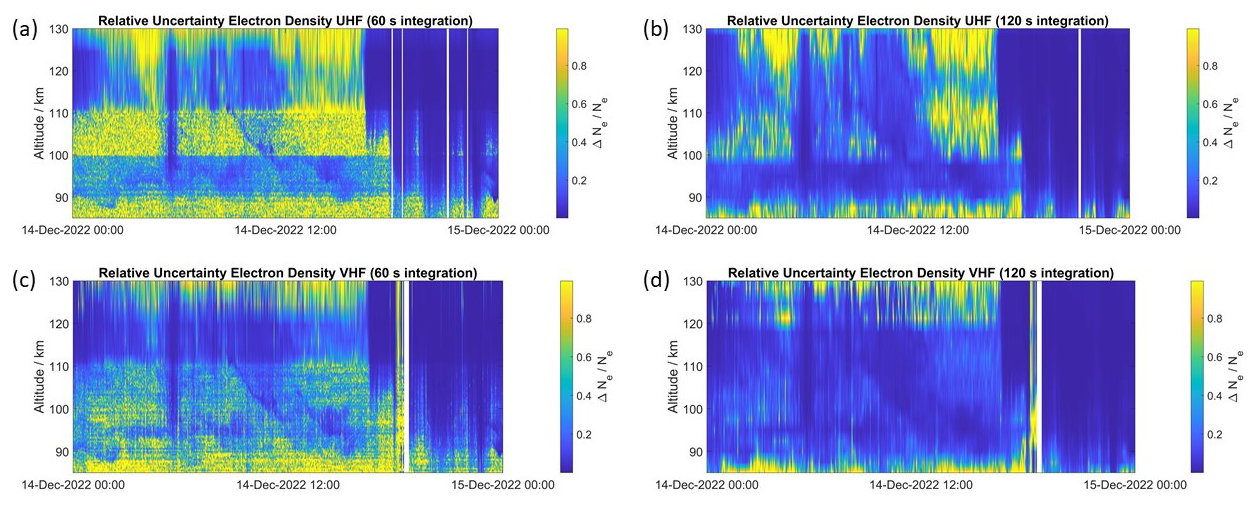
Figure 7 Relative uncertainty of electron density $\mathrm{\Delta }{N}_{\mathrm{e}}/N_{\mathrm{e}}$ for (a) EISCAT, (b) UHF, and (c, d) VHF measurements on 14 December 2022. (a, c) The “standard” case with 60 s integration windows and very high altitude resolution up to 110 km and (b, d) the analysis settings applied in this paper with 120 s integration and reduced altitude resolution are distinguished.

The relative electron density uncertainty $\mathrm{\Delta }{N}_{\mathrm{e}}/N_{\mathrm{e}}$ for the standard settings is shown in Fig. 7a and c for UHF and VHF, respectively. Both instruments exhibit considerable uncertainties below 90 km altitude, presumably due to the low electron density. The most prominent feature, however, is a band of strong noise between 100 and 110 km altitude in the UHF measurements. The lower boundary of this noise band can be explained with the settings of the ISR single-frequency analysis. Below 100 km, the ion temperature T_i is not fitted but taken from an a priori model for UHF manda measurements. This limits the variability of the ISR fit and therefore reduces the uncertainty of the plasma parameters. Above 100 km, the ion temperature is also fitted; consequently, the uncertainty increases sharply above this altitude. The upper boundary of the noise band at 110 km is presumably caused by the narrow altitude gates in the standard manda analysis. Up to 110 km altitude, the standard analysis applies very narrow altitude gates of only a few hundred meters, resulting in a low SNR and the observed large uncertainties. Therefore, a sharp transition from high to low uncertainties at 110 km altitude can be observed in the VHF measurements as well.

For the adjusted measurement setting in Fig. 7b and d, which have also been applied to obtain the results in Sect. 4, the uncertainties are notably lower. However, the UHF noise band above 100 km can still be seen at times of very low electron density (compare to Fig. 2a). Due to the adjusted altitude gates, the sharp transition at 110 km altitude is no longer present. For electron densities $N_{\mathrm{e}}>{\mathrm{10}}^{\mathrm{10}}{\text{m}}^{-\mathrm{3}}$, the uncertainties are reasonably small and can be acceptable.

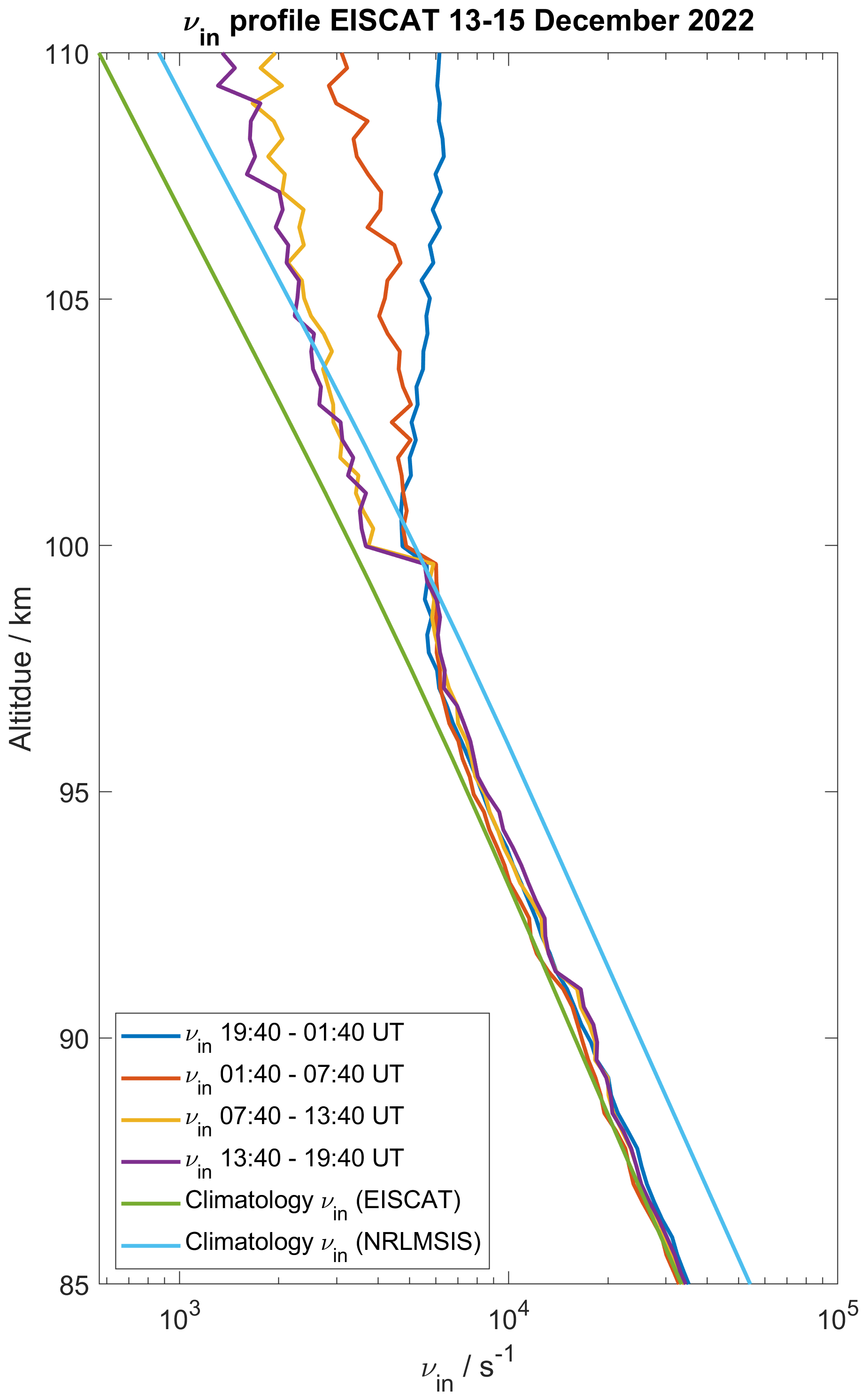
Figure 8 Equivalent to Fig. 3a but for the “standard” single-frequency EISCAT analysis settings.

A potential issue of the high uncertainties when applying the standard analysis settings is shown in Fig. 8. During the December 2022 EISCAT measurements, the collision frequency profiles are binned with local apparent solar time equivalent to Fig. 3a. A notable jump is found in all profiles at 100 km altitude. This is presumably caused by the noise band shown in Fig. 7a. Due to the adjusted analysis settings, the kink has been entirely suppressed or removed in Fig. 3.

The uncertainties for the May 2024 campaign are generally lower due to the increased electron densities and only become significant below 90 km altitude. However, applying the standard altitude gates and a 60 s integration, a discontinuity of $\mathrm{\Delta }{N}_{\mathrm{e}}/N_{\mathrm{e}}$ is found at 110 km altitude with a jump of about 50 %. Due to the generally low relative uncertainties, this would not have affected the analysis strongly and the discontinuity disappeared when applying the adjusted analysis settings.

5.2 Impact of a priori collision frequency profile

A priori parameters are relevant not only for the single-frequency fit of ISR measurements but also for the dual-frequency method. To initialize the dual-frequency ν_in fit, an a priori collision frequency profile is applied. In Fig. 3, the obtained collision frequencies for two different a priori profiles are shown. It can be seen that at low altitudes (approximately below 95 km), the fitted profiles stick very closely to the a priori profiles. We can estimate the altitudes at which the difference spectrum fit is dominated by the a priori profile from the differences between the profiles in Figs. 4a and 6a and the equivalently binned profiles obtained from fits with the EISCAT a priori profile. The profile differences for high and low N_e,95 profiles for December 2022 and the high N_e,95 profile for May 2024 are shown in Fig. 9.

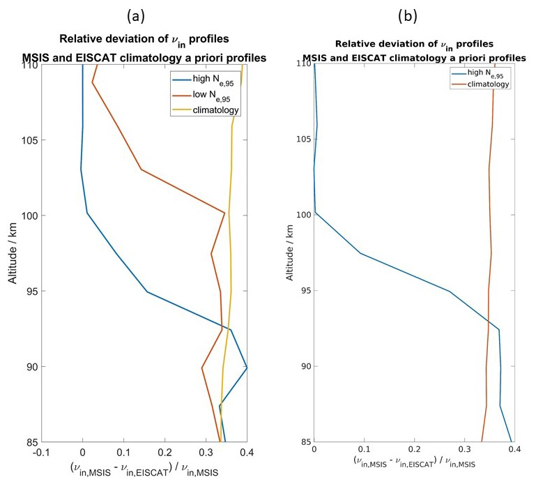
Figure 9 Deviation of ν_in profiles for a priori difference spectrum fit profiles from NRLMSIS or EISCAT climatology for (a) December 2022 and (b) May 2024.

As the difference spectrum method involves a nonlinear least-square fit of the difference in spectral amplitude, a low SNR value results in a low measurement response and the solution tends to stay much closer to the a priori profile. Although the absolute least-square errors are smaller when fitting the difference spectrum, the relative errors are much larger, causing the fit to accept the a priori profile as the solution. It can be seen in Fig. 9 that for the high N_e,95 ν_in profiles, the relative deviation of profiles obtained with different a priori profiles is considerably low above 100 km altitude. Therefore, the difference spectrum fit is not impacted by the choice of a priori profile there. Below 100 km altitude, the profiles start to deviate significantly, and below about 95 km, the profile difference is nearly equivalent to the a priori profiles. Therefore, we determined that the difference spectrum fit is a priori dominated below 95 km altitude and the obtained ν_in profiles cannot be considered reliable. This altitude is therefore shown gray-shaded in Figs. 4 and 6. The low N_e,95 profiles obtained during the December 2022 campaign show a considerable dependence on the choice of a priori profile at all altitudes. However, the profiles appear to be not completely a priori dominated above about 105 km altitude.

5.3 Energy balance of neutral uplift

An estimation of the local energy deposition rate q can be obtained from ISR electron density measurements by applying the method described by Vickrey et al. (1982). This method applies a constant empirical profile for the effective recombination rate obtained from various ionospheric and laboratory experiments. Though Gledhill (1986) showed that the effective recombination rate depends on the dominant type of particle precipitation, the method described by Vickrey et al. (1982) is applied here to estimate the local heating rate at 95 km altitude. For $N_{\mathrm{e},\mathrm{95}}>\mathrm{2}\times {\mathrm{10}}^{\mathrm{10}}{\text{m}}^{-\mathrm{3}}$, the local heating rate at 95 km altitude is $q>\mathrm{0.88}\mathrm{\mu }\mathrm{W}{\mathrm{m}}^{-\mathrm{3}}$. The height-integrated energy deposition between 90 and 110 km altitude reaches levels of approximately $Q\sim \mathrm{3}\mathrm{mW}{\mathrm{m}}^{-\mathrm{2}}$.

In order to assess the neutral uplift visible in the blue Δn_n profile shown in Fig. 4b, we also calculate the energy density required for the uplift. We calculate the difference in total potential energy for the neutral particle density profiles n_n,1 (high N_e,95 conditions) and n_n,2 (low N_e,95 conditions).

$$\begin{array}{}\text{(2)}& \begin{array}{rl}\mathrm{\Delta }E& =\underset{\mathrm{90}\mathrm{km}}{\overset{\mathrm{110}\mathrm{km}}{\int }}\left(n_{\mathrm{n},\mathrm{1}}-n_{\mathrm{n},\mathrm{2}}\right)\cdot \mathrm{29}\text{u}\cdot g\cdot h\text{d}h\\ & \approx \left(\mathrm{1.12}\pm \mathrm{2.92}\right)\text{kJ}{\text{m}}^{-\mathrm{2}}\end{array}\end{array}$$

This assumes a mean particle mass of 29 atomic mass units. At the above-calculated height-integrated energy deposition rate, it would take approximately 100 h of particle precipitation to deposit the energy for the observed uplift. So for the presented measurements, it is unreasonable that the observed median uplift is caused by particle precipitation. However, the uncertainties in Fig. 4b influence the calculation of the energy balance in Eq. (2) quite significantly, causing energy uncertainties of $\pm \mathrm{2.92}\mathrm{kJ}{\mathrm{m}}^{-\mathrm{2}}$. The uncertainties are therefore far larger than the median energy difference calculated in Eq. (2). This means that though the ion-neutral collision frequency profiles in Figs. 3, 4a, and 6a can be inferred with reasonable uncertainty, the physical impact of these uncertainties is quite major. Therefore, a considerably higher accuracy of the difference spectrum ν_in measurements is required before quantitative implications can be drawn.

5.4 Reaction time of the atmosphere

Another point that needs to be considered is the reaction time of the atmosphere gas to the heating due to particle precipitation. For a long reaction time, the binning of ν_in profiles with Q_P is not justified and the delay of the neutral uplift would need to be considered. This is especially important for the December 2022 measurements with strong fluctuations in the particle precipitation rate. We estimate the vertical neutral wind induced by the particle precipitation heating at 100 km altitude following Hays et al. (1973), Kurihara et al. (2009), and Oyama et al. (2012).

$$\begin{array}{}\text{(3)}& U_z={\displaystyle \frac{q}{\mathit{\rho }\left(c_p\frac{\mathit{\delta }T}{\mathit{\delta }z}+g\right)}}\end{array}$$

The above-estimated $q\sim \mathrm{0.88}\mathrm{\mu }\mathrm{W}{\mathrm{m}}^{-\mathrm{3}}$ is applied here. The neutral mass density ρ, the specific heat capacity at constant pressure c_p, and the vertical neutral temperature gradient $\mathit{\delta }T/\mathit{\delta }z$ are obtained from the NRLMSIS model. This results in vertical winds of $U_z\sim \mathrm{3.6}\mathrm{m}{\mathrm{s}}^{-\mathrm{1}}$. The average vertical uplift of a particle can be estimated from the energy difference in Eq. (2) as $\mathrm{\Delta }h=\mathrm{\Delta }E/\left(N_{\mathrm{n}}\cdot \mathrm{29}\text{u}\cdot g\right)$ with the height-integrated particle density $N_{\mathrm{n}}\sim \mathrm{3.75}\times {\mathrm{10}}^{\mathrm{23}}{\text{m}}^{-\mathrm{2}}$. It should be noted that N_n at 90 to 110 km altitude is nearly equivalent for all neutral density profiles including the climatology NRLMSIS profile. Considering the large uncertainty of the energy difference calculation, the possible average uplift ranges from about 6 to 19 km assuming the energy differences from Eq. (2) (larger than the median). The vertical velocity obtained from Eq. (3) results in a reaction time of approximately 27–88 min. Though the majority of $N_{\mathrm{e},\mathrm{95}}>\mathrm{2}\times {\mathrm{10}}^{\mathrm{10}}{\text{m}}^{-\mathrm{3}}$ conditions during the December 2022 campaign occurred in one interval several hours long during the night from 14 to 15 December, a reaction time of ∼90 min would definitely impact the analysis presented in this paper. Additionally, Grandin et al. (2024) showed that the typical duration of auroral precipitation events is around 20 min and therefore slightly lower than the calculated reaction time. However, Kurihara et al. (2009) noticed that the observed reaction time is usually significantly shorter than calculated from Eq. (3). If the uplift is not caused by vertical winds but rather by a density wave, the disturbance would be transported with the wave's phase velocity, which would explain the shorter reaction time. However, the atmosphere reaction time to the particle precipitation generally needs to be considered when investigating short periods of strong particle precipitation. Due to the high uncertainty of the reaction time estimate it cannot be conclusively determined that the observed changes in the ν_in profile are caused by particle precipitation. Additionally, the lower typical duration of precipitation events suggests that other mechanisms contribute as well, even if particle precipitation is the main driver. It should also be noted that the vertical wind is an estimate and not directly observed, so all interpretations should be considered with care.

5.5 Vertical wind due to tilted isobars

Our measurements do not conclusively prove that the observed neutral density changes are caused by neutral uplift due to particle precipitation heating. Since the atmospheric reaction time from the neutral uplift estimated in the previous section is presumably slightly too long, alternative explanations have to be considered.

Oyama et al. (2008) discussed the impact of tilted isobars due to localized heating events. For localized heating events, such as particle precipitation, the isobars given by the barometric formula are tilted with respect to geographic altitude. Hence, zonal and meridional winds along the isobars have a geographically vertical component. Oyama et al. (2008) showed that this vertical wind component is generally of the order of a few m s⁻¹ but can be significantly larger for strong horizontal temperature gradients. Therefore, the vertical wind due to zonal and meridional winds along tilted isobars is at least of the same order as the uplift calculated in the previous section.

It should be noted that though the geomagnetic heating due to particle precipitation or Joule heating (see Sect. 5.7) causes the tilt of the isobar, vertical advection is not necessarily correlated with the particle precipitation observed with the EISCAT radar. In Oyama et al. (2008), the heating event took place 80 km from Tromsø, but if the horizontal wind direction over Tromsø is oriented toward the heating source, an upward vertical wind component is observed.

5.6 Atmospheric tides

Atmospheric tides are an important forcing mechanism of the MLT region (Lindzen, 1979; Becker, 2017). Neutral wind measurements from the Tromsø meteor radar were analyzed (Hall and Tsutsumi, 2013) to assess the tidal activity during the time of the above-described EISCAT campaigns. Technical details for this type of meteor radar can be found in Holdsworth et al. (2004). The Tromsø meteor radar is part of the Nordic Meteor Radar Cluster, which permits obtaining spatially resolved winds covering the same observation volume as EISCAT (Stober et al., 2021a; Günzkofer et al., 2023a). The meteor radar provides measurements of the neutral wind velocities at approximately 70–110 km altitude with a time resolution of 1 h and an altitude resolution of 2 km when derived using the retrieval methods described in Stober et al. (2022). Atmospheric tides are derived by applying an adaptive spectral filter (ASF) (Baumgarten and Stober, 2019; Stober et al., 2020). The ASF is designed to determine different tidal modes using rather short windows covering only one to two oscillations for each tidal mode, which makes the method ideal for such campaign-based datasets. The performance and applicability of the ASF were already successfully demonstrated by leveraging observations from EISCAT and the Nordic Meteor Radar Cluster (Günzkofer et al., 2022).

At high latitudes, the vertical propagation of diurnal tides is inhibited. However, upward-propagating semidiurnal tides gain large amplitudes and are the dominant tidal mode up to about 120 km altitude during most months of the year (Andrews et al., 1987; Nozawa et al., 2010; Stober et al., 2021b; Günzkofer et al., 2022). Atmospheric tides are commonly considered to have an important impact on the neutral density in the lower thermosphere (Lieberman and Hays, 1994; Qian and Solomon, 2012; Truskowski et al., 2014; Maute et al., 2022; Yue et al., 2023). However, tides are most commonly measured as neutral wind or temperature oscillations with meteor radars and lidars. Figure 10 shows the amplitude of the semidiurnal atmospheric tide in the zonal and meridional neutral winds as measured with the Tromsø meteor radar.

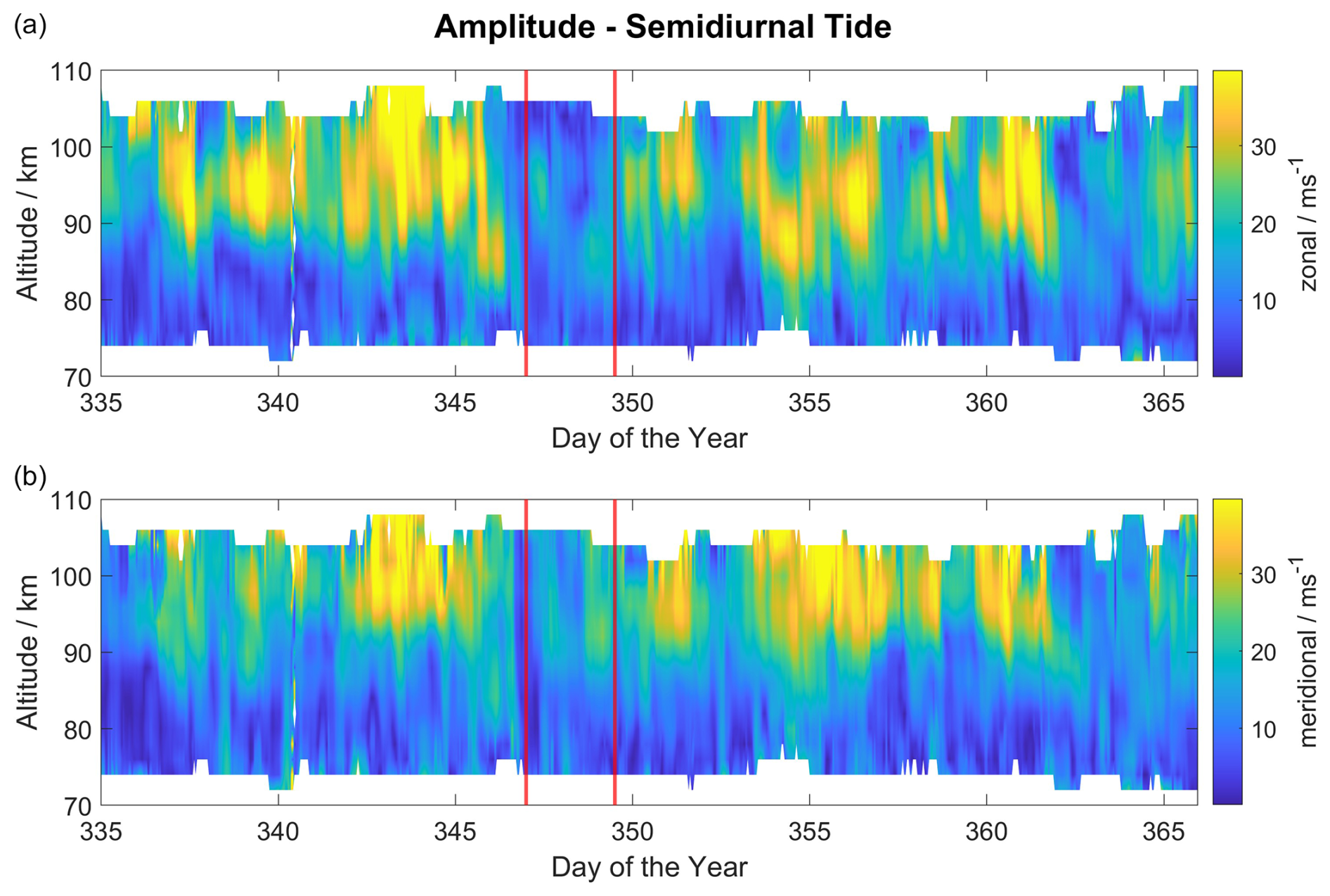
Figure 10 Amplitude of the semidiurnal tide in zonal (a) and meridional (b) neutral winds measured with the Tromsø meteor radar. The vertical red lines mark the beginning and the end of the EISCAT Geminids campaign during December 2022.

The semidiurnal tide reached amplitudes of up to $\sim \mathrm{40}\mathrm{m}{\mathrm{s}}^{-\mathrm{1}}$ during December 2022 in both zonal and meridional wind. This is close to the values given by the Global Scale Wave Model climatology (Hagan and Forbes, 2003). However, during the EISCAT Geminids campaign, the tidal amplitude was notably lower and reached amplitudes of only $\sim \mathrm{20}\mathrm{m}{\mathrm{s}}^{-\mathrm{1}}$ and lower. Since the classical tidal theory usually applies logarithmic pressure units, neutral density oscillations are not directly described by the tidal equations (Andrews et al., 1987). However, measurements indicated that typical values for collision frequency and neutral density oscillations due to tidal forcing at midlatitudes are of the order of a factor of 2 (Waldteufel, 1970; Monro et al., 1976). The neutral density variations observed in Figs. 4b and 6b are in a range of a factor of 2 to 5 at 95–110 km altitude. Hence, at the lower measurement altitudes, the observed neutral density variations are comparable to the possible variations from tidal forcing. However, considering that semidiurnal tidal amplitudes decrease at higher latitudes and that the tidal amplitudes were generally decreased during the measurement campaign, it seems unlikely that the tidal forcing caused neutral density variations of the order of a factor of 2. This suggests that the relative importance of atmospheric tides for the ion-neutral collision frequency profile is small.

5.7 Joule heating impact

Assuming our interpretation that the observed changes in the ion-neutral collision frequency profile are the result of a neutral uplift due to ionospheric heating, other heating mechanisms need to be discussed. One of the most important heating mechanisms in the lower thermosphere is Joule heating due to Pedersen currents, which has been shown to cause significant neutral uplift in the lower thermosphere (Deng et al., 2011). The maximum Joule heating occurs at the Pedersen conductivity maximum at approximately 120 km altitude. The Joule heating drops rapidly at lower altitudes, though there might still be a considerable impact at 100–110 km altitude. For the December 2022 EISCAT measurements, the geomagnetic activity was consistently low with Kp ≤2. Recent investigations showed that for such low geomagnetic activity, the Joule heating at 110 km altitude reaches values of the order of 0.01 µW m⁻² (Baloukidis et al., 2023; Günzkofer et al., 2024), which is considerably lower than the estimated particle precipitation heating rates. However, the local geomagnetic activity over Tromsø can be higher than the global Kp index suggests, as can be seen from the SME index in Fig. 1. The local K index over Tromsø (Frøystein and Johnsen, 2024) reached values up to K=4.

For May 2024, where the maximum geomagnetic activity reaches Kp=6, the Joule heating at 110 km altitude can reach 0.1 µW m⁻² or even higher values (Baloukidis et al., 2023; Günzkofer et al., 2024). Additionally, the increased ionization due to particle precipitation increases the Pedersen conductivity and consequently the Joule heating. Joule heating contributes to the upwelling of the neutral atmosphere above about 120 km (Deng et al., 2011). At 100 km altitude, Joule heating might contribute to ionospheric heating, especially for high geomagnetic activity. However, the Pedersen conductivity is rapidly reduced below the altitude of its maximum. Therefore, particle precipitation is supposed to be the stronger heating mechanism at these altitudes according to the literature. However, for strong precipitation conditions like during the investigated measurements, the common Kp index estimate of Joule heating might be insufficient. Since the exact cause of the neutral density increase cannot be determined, a potential impact of Joule heating should be considered.

5.8 Rigid-sphere, Maxwell, and resonant collisions

The neutral particle density differences Δn_n shown in Figs. 4b and 6b are calculated from the ν_in profiles by applying Eq. (1). It is assumed that ion-neutral collisions can be described as rigid-sphere collisions (Chapman, 1956). Another collision model often applied assumes Maxwell collisions of the ions and polarized neutrals (Schunk and Walker, 1971). However, it has been shown that the calculated neutral density profile is not impacted by the choice of the collision model for these altitudes (Günzkofer et al., 2023b). Therefore, applying the more simple rigid-sphere model is justified here. The plasma density n_i in Eq. (1) is commonly neglected for the calculations. This is reasonable at all altitudes, since even for the highest investigated altitudes at 110 km, the neutral density is larger than the plasma density by at least a factor of 10⁶.

Both approaches mentioned so far, rigid-sphere and Maxwell collisions, are so-called non-resonant collisions. However, resonance effects have to be considered for collisions between neutral particles and their first positive ions (in the MLT region, mainly O₂ and O₂+). Following Ieda (2020), O₂ and O${}_{\mathrm{2}}^{+}$ predominantly dominate at ion temperatures T_i>600 K (assuming ion and neutral temperatures to be the same in the MLT region). For the May 2024 measurements, T_i>600 K was not reached at altitudes up to 110 km according to the UHF measurements (for which T_i is fitted above 100 km). However, the December 2022 UHF measurements showed T_i>600 K at 110 km for about 5 % of all measurements. It should be noted that these T_i>600 K measurements were entirely obtained during times of very low electron density and are hence subject to the remaining UHF data noise shown in Fig. 7b. Also, as already noted by Ieda (2020), since O₂ only makes up about 20 % of the neutral particles in the MLT region, the impact on the total collision frequency is limited. Nonetheless, we repeated the analysis in Sect. 4 and included resonant collisions. The neutral density difference Δn_n profiles shown in Fig. 4b were unaffected by this recalculation since no T_i>600 K conditions fell into the $N_{\mathrm{e},\mathrm{95}}>\mathrm{2}\times {\mathrm{10}}^{\mathrm{10}}{\text{m}}^{-\mathrm{3}}$ domain. Hence, we conclude that the obtained T_i>600 K values are the result of low SNR ratios, and, as already stated by Ieda (2020), resonant collisions can be neglected at altitudes up to 110 km.

5.9 The difference spectrum method

The difference spectrum method is described in Grassmann (1993b) and the limits of its application have been discussed in Günzkofer et al. (2023b). The main uncertainty of the difference spectrum method is related to the required β parameter that is applied to compensate for technical differences between the UHF and VHF ISR when combining the two spectra. The β parameter should be determined at F-region altitudes where the ionosphere can be assumed to be collisionless. However, due to the different beam shapes of the UHF and VHF radars, the β parameter in fact varies slightly with altitude (Günzkofer et al., 2023b). The manda pulse code applied for both EISCAT campaigns analyzed in this paper allows measurements up to 200 km altitude, which is below the F layer, and thus the β parameter can only be derived with some margin of uncertainty. In this study, the β parameter is determined at this maximum altitude where the ratio of ion-neutral collision to gyro-frequency is approximately 0.02, taking into account the climatological average. This is a drawback of the manda pulse code compared to the beata mode, which covers higher altitudes above 200 km, and hence the assumption of a collisionless plasma is better satisfied at these higher altitudes, making the analysis more resilient for this EISCAT mode.

5.10 Quantification of particle precipitation

To investigate the impact of particle precipitation on the ν_in profile, we binned the obtained collision frequency measurements with the electron density at 95 km altitude, N_e,95. Applying N_e,95 as a quantification for the particle precipitation impact assumes that it is the dominant ionization mechanism at this altitude. Following Fang et al. (2010, 2013), the particle precipitation impact at 95 km altitude is mainly carried by electrons with energies of about 10–100 keV and protons with energies of about 1 MeV. For particle precipitation energy rates of 1 mW m⁻², the ionization rates due to particle precipitation are of the order of ${\mathrm{10}}^{\mathrm{10}}{\text{m}}^{-\mathrm{3}}{\text{s}}^{-\mathrm{1}}$. Especially during December, when the solar elevation angle is very low at high northern latitudes, this should exceed the photoionization rate (Baumjohann and Treumann, 1996). The solar elevation angle is considerably higher in May at the Tromsø geographic latitude. Therefore, photoionization rates during daytime measurements of the May 2024 EISCAT campaign cannot be neglected and the quantification of the particle precipitation impact by N_e,95 introduces additional uncertainties.

Our analysis is based on steady-state conditions during the ISR experiment dwell time of 120 s, which is presumably only partly justified as the energy transfer happens on much shorter timescales for individual collisions. However, this seems to be justified at least statistically for the ensemble of all precipitating particles within the observation volume. Most ionospheric dynamics take place on larger timescales, but it has been shown for frictional heating processes that shorter scales do contribute as well (Brekke and Kamide, 1996). A shorter dwell time for the radar experiments is not feasible for observing E-region dynamics due to the lower total electron densities at the transition region between D and E regions.

In Fig. 2a, it can be seen that occasionally the electron density below 100 km appears to be higher than at higher altitudes. In these cases, the $N_{\mathrm{e},\mathrm{95}}>\mathrm{2}\times {\mathrm{10}}^{\mathrm{10}}{\text{m}}^{-\mathrm{3}}$ ion-collision frequency profiles may be affected by the data noise issues shown in Fig. 7 that cause the enormous uncertainty of the $N_{\mathrm{e},\mathrm{95}}<\mathrm{1}\times {\mathrm{10}}^{\mathrm{10}}{\text{m}}^{-\mathrm{3}}$ profile in Fig. 4a. However, only for about 0.5 % of the total measurements was it found that $N_{\mathrm{e},\mathrm{95}}>\mathrm{2}\times {\mathrm{10}}^{\mathrm{10}}{\text{m}}^{-\mathrm{3}}$, while the electron density at 105 km is $N_{\mathrm{e},\mathrm{105}}<\mathrm{1}\times {\mathrm{10}}^{\mathrm{10}}{\text{m}}^{-\mathrm{3}}$. We repeated the analysis in Sect. 4 excluding all measurements with $N_{\mathrm{e},\mathrm{95}}>N_{\mathrm{e},\mathrm{105}}$ but obtained nearly identical results.

6 Conclusions

We studied the variation of the ion-neutral collision frequency, measured by dual-frequency ISR observations during two measurement campaigns, one during the Geminids meteor shower in December 2022 and another during a solar energetic particle event in May 2024. We found a distinct diurnal variation of the ν_in profile, which indicates a significant deviation from the climatology depending on the time of the day. Applying the electron density at 95 km altitude N_e,95 as a quantification for the strength of particle precipitation, we showed that there is a connection of the ion-neutral collision frequency at 90–110 km altitude and particle precipitation. Below about 100 km altitude, the ion-neutral collision frequency decreases for large N_e,95, while above about 100 km altitude, ν_in is increased. However, the collision frequency profiles measured under low-electron-density conditions showed large uncertainties and therefore only the measurements for high ionization can be assumed to be reliable.

Assuming a rigid-sphere ion-neutral collision model, the difference of the neutral particle density profiles n_n for $N_{\mathrm{e},\mathrm{95}}>\mathrm{2}\times {\mathrm{10}}^{\mathrm{10}}{\text{m}}^{-\mathrm{3}}$ from the climatology was calculated. Our interpretation of the ν_in profile variation for changing N_e,95 is that the heating due to the precipitating particles causes an upwelling of the neutral atmosphere. This is also observed in a second ISR measurement campaign that was specifically conducted during an SEP event and therefore exhibits continuously high N_e,95 values. We found that during the SEP event, the ion-neutral collision profiles resembled the profiles measured for the highest N_e,95 values of the Geminids campaign. The neutral particle density profiles measured during the SEP event exhibit a similar decrease or increase in neutral particle density though the uplift is shifted to lower altitudes by about 2–3 km. We interpret this as the result of a higher energy of the precipitating particles. Changes in the ion-neutral collision frequency profile caused by upwelling due to ionospheric heating have been previously reported and discussed (Nygrén, 1996; Oyama et al., 2012). However, we discussed alternative explanations for the observed changes in the ion-neutral collision frequency like Joule heating and atmospheric tides as well as data quality issues due to the generally low electron density in the MLT region. Neutral winds along tilted isobars have been shown to cause vertical winds of a similar velocity as the estimated neutral uplift due to particle precipitation heating (Oyama et al., 2008). The observed collision frequency profiles cannot be conclusively linked to a neutral uplift caused by particle precipitation heating, though a correlation has been shown in this paper.

We estimated the physical impact of the inferred ion-neutral collision frequency profiles and found a major impact of the ν_in uncertainties on the energy balance of the observed atmospheric uplift. This indicates that exact quantitative conclusions have to be drawn carefully since both physically possible and impossible (in terms of energy balance) atmospheric changes are within the measurement uncertainty range. Furthermore, we performed a sensitivity analysis highlighting how different climatology profiles used to initialize the dual-frequency fitting can impact the ν_in profiles for low SNR measurements often related to low electron densities. This revealed that the ν_in profiles obtained with the difference spectrum method are considerably impacted by the a priori collision profile below 95 km altitude. This also needs to be considered when drawing conclusions about the observed neutral uplift.

This study has shown how neutral atmosphere dynamics in the ionospheric dynamo region can be investigated by ion-neutral collision frequency measurements with dual-frequency ISRs. Though such measurements are rare so far, they provide a promising method to investigate the impact of ionospheric processes on the neutral atmosphere.

Future dual-frequency ISR campaigns should aim to observe different storm conditions in addition to SEP events, e.g., following coronal mass ejections and unusually strong substorms and super-storms. Similarly, the impact of other ionospheric heating mechanisms, especially Joule heating, on the neutral atmosphere can be studied. Dual-frequency ISR campaigns following strong geomagnetic storms, as they can be expected during the current solar maximum, could show a similar upwelling of the neutral atmosphere as caused by particle precipitation. Since the neutral atmosphere above 100 km altitude is generally difficult to measure, dual-frequency ISR measurements might also give further insight into seasonal changes, such as those caused by variations of tidal and gravity wave activity around the spring and fall equinoxes. Lastly, the difference spectrum method has been applied to multiple dual-frequency ISR campaigns so far and appears to be a reliable analysis method for these experiments. However, a definite verification of the method is not possible with dual-frequency measurements. An all-time unique opportunity for triple-frequency ISR measurements might be possible when the EISCAT UHF and VHF ISRs are operated together with the upcoming EISCAT_3D radar (McCrea et al., 2015). The EISCAT_3D radar will be operated at nearly the same radar frequency as the EISCAT VHF ISR, but the beam shape will resemble that of the UHF ISR, which permits the quantification of the suspected impact of the different beam shapes and the corresponding differences in the observation volumes between the VHF and UHF ISRs.