A critical review and presentation of the complete, historic series of K indices as determined at Norwegian magnetic observatories since 1939

The complete existing time series of K indices from Norwegian observatories in Tromsø (TRO), Dombås (DOB) and Bear Island (BJN) has been digitized. The digitized time series are continuous, spanning from 1939 (DOB) and 1947 (TRO) until 1998. Today, Tromsø Geophysical Observatory manages geomagnetic observations throughout Norway and K indices are calculated in real time with a fully automatic, in-house method. In this paper, the old hand-scaled and new automatic time series of K indices are reviewed and compared for the intervals where they overlap. Our analysis confirms that the digital K-index series is a valid continuation of the old series, at least in the auroral zone. Since 1939, three K-index derivation methods have been applied to Norwegian magnetic observatory data. These are traditional hand-scaling, the method developed by the Finnish Meteorological Institute and an in-house method. Here, we compare the tree methods. It becomes clear that each method has both strengths and weaknesses. Importantly, differences arise when calculating the quiet-day variation, especially during periods of consecutive disturbed nights at auroral latitudes. By analysis of the K-index frequency distributions for six stations in mainland Norway and on Svalbard, we find that the lower limit for K=9 of 2000 nT is too high for TRO and that for K=9 of 750 nT is possibly too low at DOB. The assumption that the variation in H is greater than that in D, which makes it possible to calculate K from the magnetic H component only, is investigated, and it is shown that the assumption is indeed only valid for auroral stations. In total, this paper presents all K indices derived from Norwegian observatories since the 1930s until today, the used derivation methods and the long historic time series as a whole, and thus it enables critical use of the indices for future scientific work. Finally, we present the complete Ak time series for the Norwegian observatories as well as a spectral analysis.

1 Introduction

Today, Tromsø Geophysical Observatory (TGO) at UiT The Arctic University of Norway takes care of geomagnetic observations throughout Norway, spanning subauroral, auroral and polar cap latitudes. The first systematic geomagnetic measurements in Norway started with Kristoffer Hansteen and the establishment of the Kristiania Magnetic Observatory in 1843 (Wasserfall, 1941). The time series from this observatory does not include continuous registrations of the magnetic elements, but rather two absolute measurements every day. Kristian Birkeland introduced variometers in geomagnetic work in Norway. Such instruments were installed during both of his expeditions to northern Norway in 1899–1900 (Birkeland, 1901) and 1902–1903 (Birkeland, 1908).

From 1912, the Haldde Observatory in Alta was operated as a permanent “magnetic–meteorological” observatory under the leadership of Ole Andreas Krogness, one of Birkeland's former students. The Haldde Observatory performed continuous magnetic registrations until it was closed down in 1926 (Krogness and Tönsberg, 1936). The Haldde time series was continued at the auroral observatory in Tromsø (TRO) from 1928, after a temporary period at the Geophysical Institute nearby. To get context for the work at Haldde from a subauroral station, the Dombås Magnetic Observatory (DOB) was established in 1916. Today this is the oldest magnetic observatory in operation in Norway.

During the International Polar Year (IPY) 1932–1933, Polish researchers set up a magnetic observatory on Bear Island (BJN). The measurements were continued by the Auroral Observatory in Tromsø with the assistance of the Meteorological Institute. With an intermission during World War II (1941–1945), the measurements still continue today.

Thus, measurements at Norwegian stations DOB, TRO and BJN are closing in on a century of magnetic measurements stretching from subauroral to auroral latitudes. Prior to the digital era, efficient ways of providing measurements were needed to allow workers to study and combine data from multiple locations away from their own. The efficient way of doing this was to compile indices from the raw magnetic measurements and disseminate them via yearbooks and exchange networks of these. A wide range of indices have been used for various purposes and analysis aims. Still, today, even with full access to sub-minute-resolution geomagnetic data over the Internet, indices have maintained their popularity. Even if the true data usually give a more accurate and physically interpretable picture of the geomagnetic activity and studies such as Menvielle et al. (2011) warn about the validity at high latitudes owing to considerations regarding the magnetic energy density of the magnetic variations, the K index in particular is widely used.

Bartels et al. (1939) introduced the K index, and through his and co-workers' efforts it became the de facto standard measure for local geomagnetic disturbances among magnetic observatories worldwide. In this paper we present efforts made to digitize time series of geomagnetic activity (K index) at three magnetic observatories in Norway as far back in time as possible. We document the sources of where these data have been found, and based on these we present the time series, including a time series analysis. We analyze the transition from manual to automatic scaling of the K index to ensure that the time series can be assumed to be continuous. Furthermore, we investigate the difference between the IAGA-endorsed Finnish Meteorological Institute (FMI) method for K-index scaling and an in-house method, termed the TGO method. We find that, at least for auroral latitudes, the TGO method does not perform worse than the FMI method.

Through the work presented in this paper, we make a complete historic time series of geomagnetic activity as described using the K index available to the scientific community. By discussing and analyzing the methods that have been used and the transition to the digital era, we pave the way for critical, scientific application of the time series.

Magnetometer stations in Norway

Currently, TGO operates a total of 17 variometer stations and observatories, from Karmøy in the southwestern part of Norway to Ny-Ålesund on Svalbard. All 17 stations are listed in Table 1, along with their coordinates, the station type and the first year(s) of operation. A map of the station locations is shown in Fig. 1. The map also indicates the location of the historic observatory at Halddetoppen, marked in green.

Table 1 Information on the geomagnetic observatories and stations in Norway. Corrected geomagnetic coordinates and L values are from the 2022 IGRF/DGRF model (NASA Goddard Space Flight Center, corrected geomagnetic coordinates and IGRF/DGRF model parameters, https://omniweb.gsfc.nasa.gov/vitmo/cgm.html, last access: 21 October 2022).

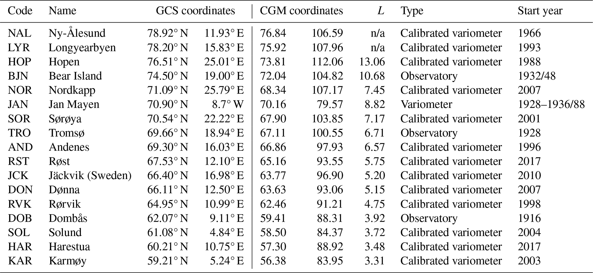
n/a: not applicable

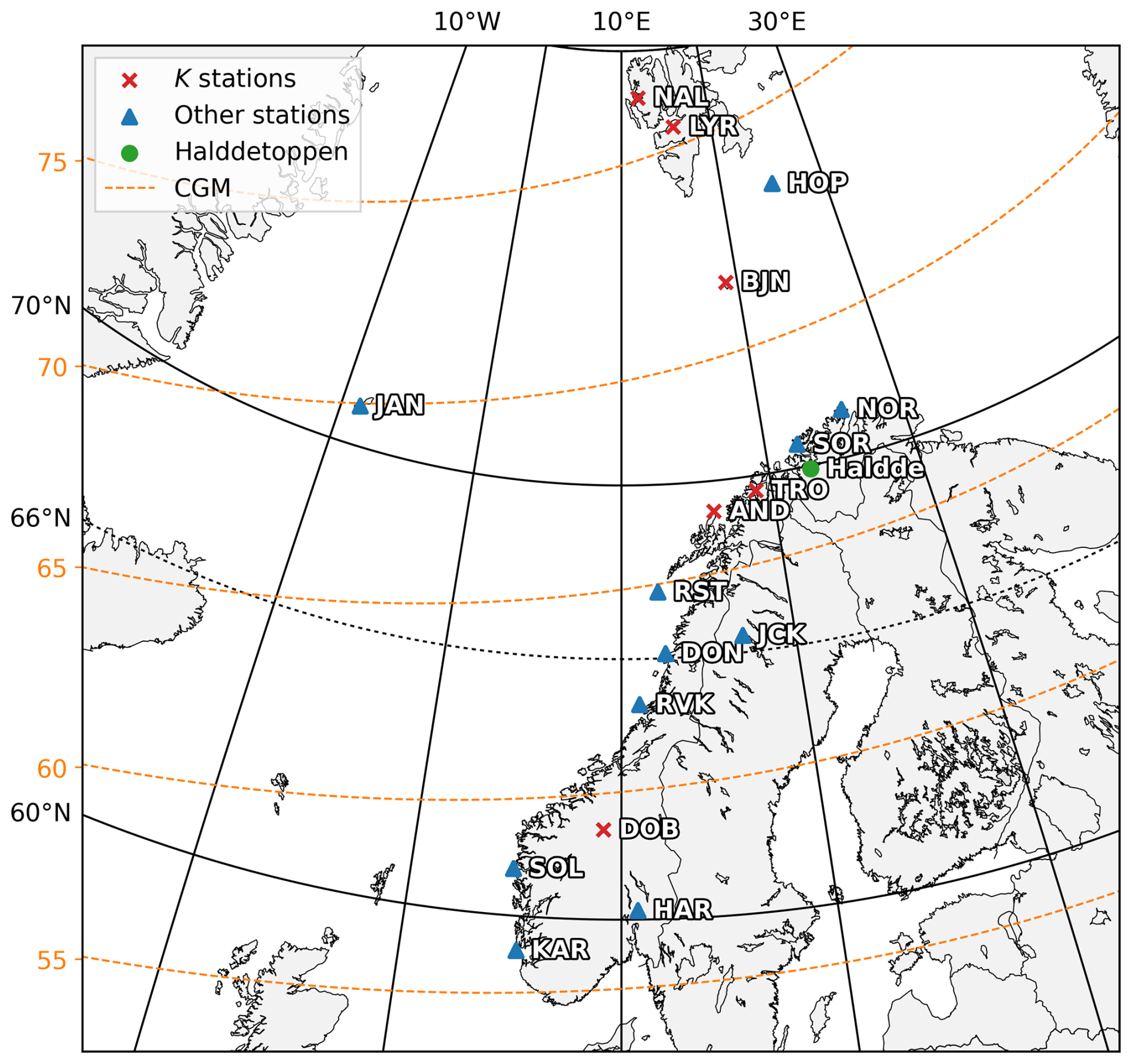
Figure 1 Map of Norwegian magnetic stations. K-index stations are marked with red crosses. The remaining stations are marked with blue triangles. The historic observatory at Halddetoppen is marked with a green circle. CGM latitudes are marked with orange dashed lines. See Table 1 for details.

The K index

The K index (Bartels et al., 1939) is a station-specific measure of the geomagnetic disturbance, or rather disturbance range, over a 3 h interval. The K index only includes the geomagnetic disturbance and not quiet-day variations (Matzka et al., 2021). It ranges from K=0 to K=9 on a quasi-logarithmic scale. The value is calculated for the intervals 00:00–03:00, 03:00–06:00, …, 21:00–24:00 UT. Previously, all components D, H and Z were used when calculating K. Today, only D and H are used, partly to remove the effect of induced underground currents (Mayaud and IAGA, 1967). Before a complete set of directions for calculating K was published by Mayaud and IAGA (1967), different methods for hand-scaling K had been used at different observatories. A rigorous description of the method for hand-scaling is given by Mayaud and IAGA (1967), but in short the steps can be described as follows.

The first step is to estimate the quiet-day variation S_q or quiet-day curve (QDC). When the QDC is found, the K values for components H and D or X and Y on each 3 h interval are found directly by using a customized gauge. The gauge is made to fit the ranges for each K value for the observatory (see, e.g., Fig. 5 in Mayaud and IAGA, 1967, for such a gauge). The resulting K indices, and especially the estimated QDC, will vary somewhat based on the observers, their experience and knowledge of the quiet-day variation at their observatory. However, Matzka et al. (2021) note that it is expected that the agreement between K indices derived by different experienced observers would generally be at least 80 %.

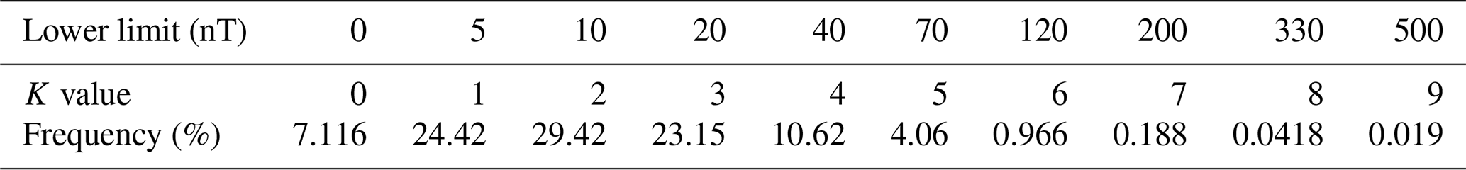
Depending on the geomagnetic latitude and therefore the amount of geomagnetic disturbance experienced at each station, the ranges for each station are adjusted to the latitude. This is done by scaling the Niemegk ranges, shown in Table 2, by a set lower limit for K=9, the K9 limit.

Table 2 Lower limits (nT) for each K value for the Niemegk observatory (Mayaud, 1980) and frequency distribution (Matzka et al., 2021).

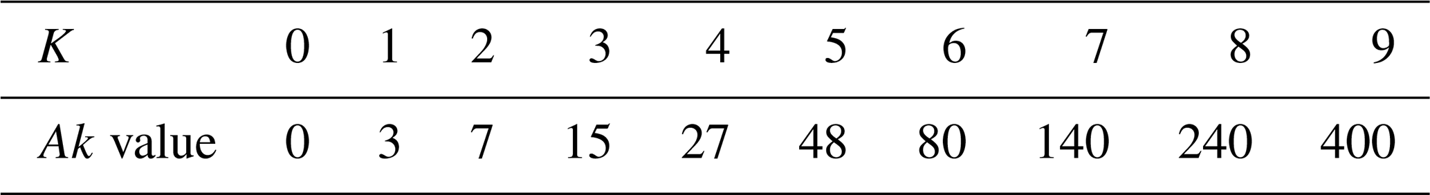
The ak index is derived from K, converting K into a linear scale (Bartels and Veldkamp, 1954; Van Sabben and IAGA, 1972). The conversion values are shown in Table 3. It is therefore possible to compute averages: daily Ak, monthly Ak and yearly Ak. These indices are useful when investigating long-term variation of geomagnetic disturbances (e.g., Nevanlinna, 2004; Nevanlinna et al., 2011).

Table 3 Conversion table for K into the ak index.

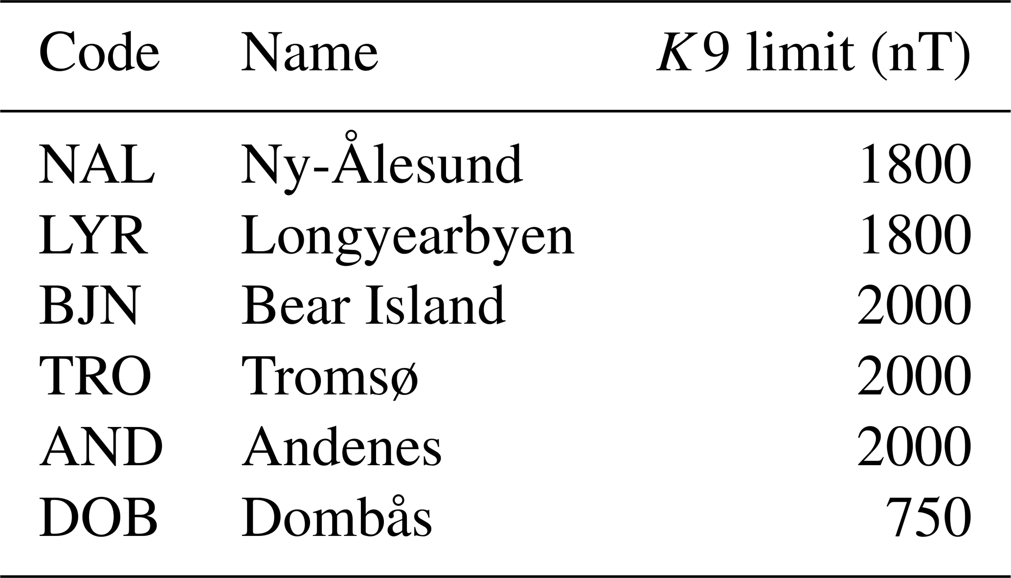
The K index is routinely calculated for six stations in Norway. These six stations are, sorted from south to north, DOB, Andenes (AND), TRO, BJN, Longyearbyen (LYR) and Ny-Ålesund (NAL). The stations are marked in red on the map in Fig. 1. K indices were first published in Norway in 1939, from the DOB observatory. From 1947 K indices were also published from the TRO observatory. K indices from TRO and DOB are calculated to this day. K indices were calculated for BJN during a short interval from 1951 to 1965 and also for the International Polar Year (1932–1933). In more recent years, i.e., in 1986, 1993 and 1996, calculation of the K index was started at LYR, NAL and AND, respectively. The calculations of K indices at LYR and NAL were started based on popular request.

Due to the large spread in geomagnetic latitude among the Norwegian K-index stations, three different K9 limits spanning the range from 750 to 2000 nT are used. The limits are presented in Table 4.

Table 4 K9 limits for the Norwegian K-index stations.

Norwegian K indices have been used in numerous studies, especially since the TGO method was implemented and the K indices were made available digitally. The studies include, to name a few, work on the aurora (Nanjo et al., 2022), work on polar mesospheric summer echoes (Bremer et al., 2000, 2001; Zeller and Bremer, 2009), GNSS disturbances and scintillation (Andalsvik and Jacobsen, 2014), thermal structures in the ionosphere, thermosphere and mesosphere (Kurihara et al., 2010) and dynamic instabilities and their relationship with geomagnetic activity (Nozawa et al., 2023).

2 The dataset, digitization and K derivation methods

2.1 K indices

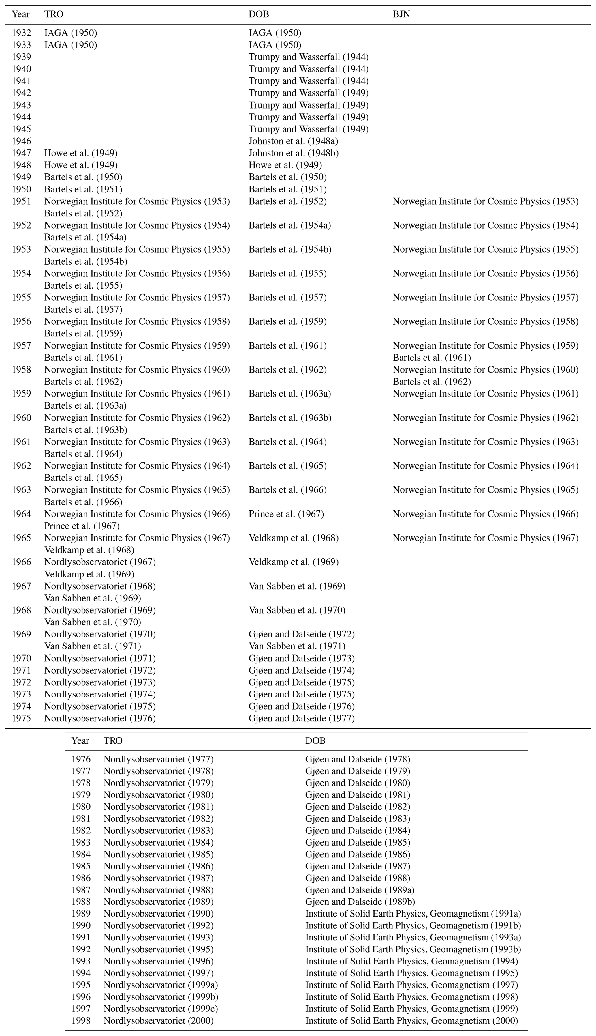
The K indices from the observatories in Tromsø, Dombås and Bear Island have been published in (1) the IATME/IAGA Bulletin no. 12 (available from the International Service of Geomagnetic Indices, IAGA, at http://isgi.unistra.fr/iaga_bulletin.php, last access: 14 October 2024) and in (2) yearbooks from the observatories in Dombås and Tromsø. All the yearbooks have been scanned and published on the TGO website (https://www.tgo.uit.no/ScanRap/GeoPhysRap.html, last access: 30 April 2025). K indices from Tromsø were submitted to IAGA from 1947, and K indices from Dombås were submitted from 1946. K indices from Bear Island were submitted only in a short interval from late 1957 to mid-1959 as a contribution to the International Geophysical Year (IGY). Indices from the International Polar Year (1932–1933) were also submitted to IAGA for all three stations.

The yearbooks from Tromsø were published by the Norwegian Institute of Cosmic Physics from 1930 to 1965 and by the Auroral Observatory (University of Tromsø) from 1966 to 1998. The observations from Bear Island were published in the Tromsø yearbooks. The yearbooks from Dombås were published by the Norwegian Institute of Cosmic Physics from 1916 to 1958, by the Geophysical Institute at the University of Bergen, Norway, from 1959 to 1988 and the Institute of Solid Earth Physics and Geomagnetism at the University of Bergen, Norway, from 1989 to 1998. No yearbook was made for DOB in the interval 1949–1951. In this period the observatory was in the process of being moved (Gjellestad et al., 1957).

The K indices from all three observatories were digitized by typing the published values into plain ASCII files. When digitizing data manually by “human hand”, it is impossible to safeguard completely against errors such as typing the wrong number. However, for this dataset it was the most convenient way owing to the large number of different table formats and page layouts in both the yearbooks and the IAGA Bulletin no. 12. Table B1 shows where the K values were published. The digitized K values were retrieved from the observatory yearbooks when the K indices were included in the yearbook for that station and year. In some years the K indices were not included in the yearbooks but rather submitted directly to the Association of Terrestrial Magnetism and Electricity (IATME, now IAGA). When digitizing these years, the K indices were obtained from the IAGA Bulletin no. 12.

The digitization of historic data and the dissemination over the Internet have gained increased popularity over the decades (e.g., Sergeyeva et al., 2021; Nevanlinna and Häkkinen, 2010). This is important in order to make valuable, historic, and often high-quality data available to a wider scientific public than only those with direct access to the original material. Therefore, the digitized Norwegian K indices have been made public through the TGO websites next to the more recently generated geomagnetic data (available at https://flux.phys.uit.no/Kindice/Manual/index.html, last access: 15 May 2025).

2.2 Digital derivation methods used in Norway

Traditional hand-scaling of magnetograms (Bartels, 1957; Mayaud and IAGA, 1967) was used to derive K for TRO from 1947 to 1991, for BJN from 1951 to 1965 and for DOB from 1939 to 1994. In addition, three digital derivation methods have been used to derive K indices in Norway. The three methods are the FMI method and two versions of an in-house method from now on referred to as the TGOe (e for “early”) and TGO methods. Brief descriptions of the three methods are presented in the following sections.

2.2.1 The FMI method

The FMI method, developed by Lasse Häkkinen at the Finnish Meteorological Institute (Sucksdorff et al., 1991), was in 1993 officially recognized as a method for deriving K by the International Association of Geomagnetism and Aeronomy (IAGA News, December 1993). In addition, it was found to be superior to the other methods considered (Menvielle et al., 1995). The FMI method was used between 1995 and 1998 to derive K at DOB (Institute of Solid Earth Physics, Geomagnetism, 1997). The FMI method FORTRAN code is available from the International Service of Geomagnetic Indices (ISGI) (K-index software, https://isgi.unistra.fr/softwares.php, last access: 15 November 2024). The C implementation is available from the FMI websites (https://space.fmi.fi/MAGN/K-index/FMI_method/, last access: 21 November 2024). The C version is newer and has been applied to data from TGO's digital flux-gate magnetometers in this study.

The FMI method is an iterative scheme based on linear elimination for calculating the K values, where the K values and QDCs for 1 d are found based on magnetograms from the previous, current and next days. Descriptions of the method are given in Sucksdorff et al. (1991) and Menvielle et al. (1995) and also by detailed examples on the FMI website (https://space.fmi.fi/MAGN/K-index/FMI_method/, last access: 21 November 2024). In short, the method can be summarized as follows. First, preliminary K indices are calculated for all eight intervals without first subtracting a QDC. These preliminary K indices are used to adjust the size of an averaging that is applied to the data before fitting of a fifth-order harmonic curve to the data, which is the preliminary QDC. Next, new K indices are calculated after subtracting this QDC. These new K indices are used for a new averaging. Finally, the last QDC is fitted to the averages; this is also a fifth-order harmonic curve. The final fitted QDC is subtracted, and the final set of K indices is calculated. This scheme is followed for both horizontal components (X and Y or D and H), and the largest value of the two in each interval is then selected.

2.2.2 The current in-house method (TGO method)

The TGO method, an automatic algorithm, was developed by Truls Lynne Hansen at the Auroral Observatory (today TGO) as a lightweight and simpler alternative to the FMI method aimed especially at real-time generation (Truls Lynne Hansen, personal communication). The TGO method is used on all six Norwegian K-index stations, and it calculates the values in real time and therefore in principle applies to any data where digital data exist. This means that K indices have been available using the TGO method for NAL since 1986, TRO since 1987, AND since 1995, LYR since 1993, BJN since 1987 and DOB since 1993. The TGO method is described below.

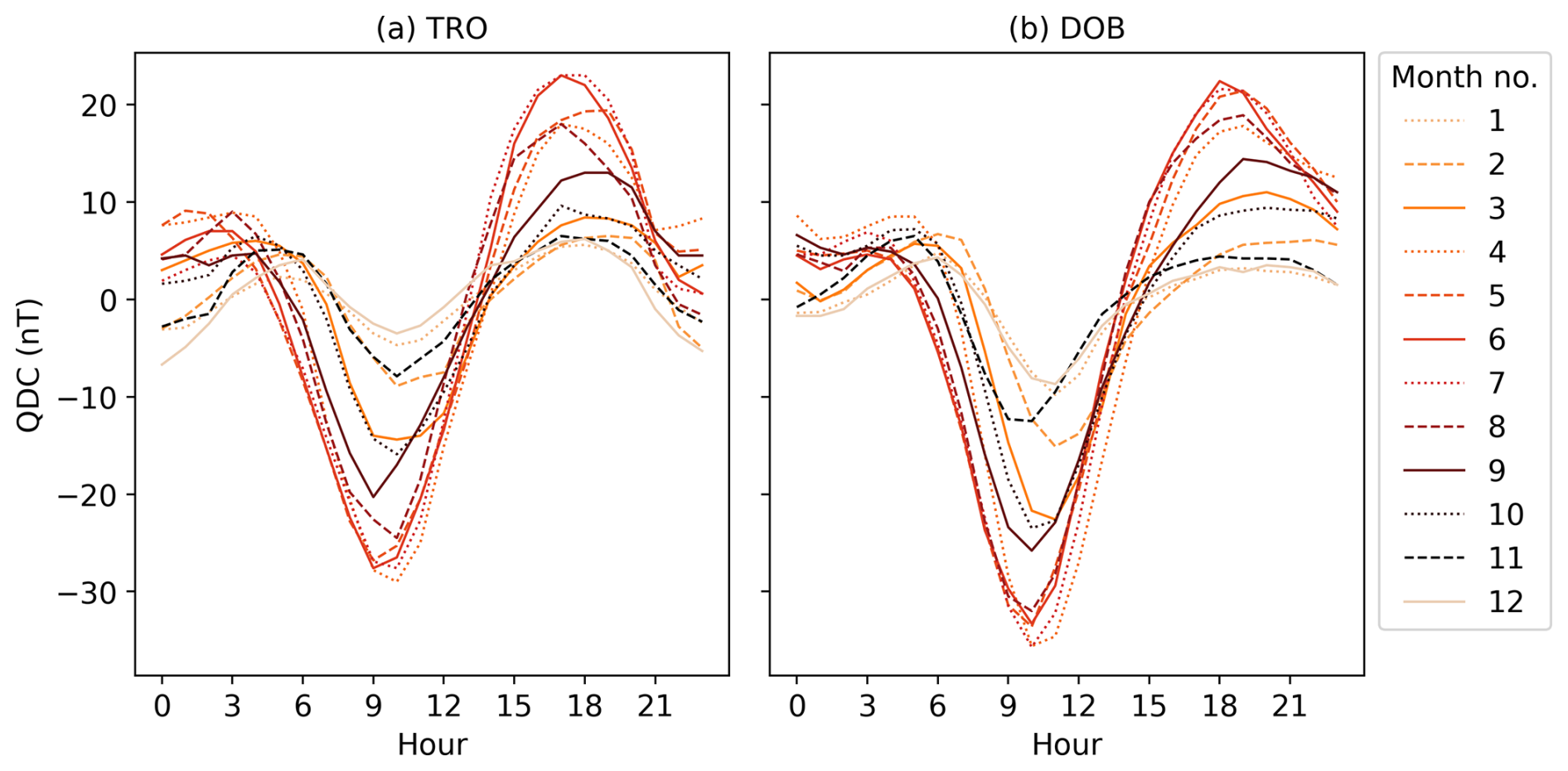
The TGO method uses the fact that the quiet-day variation is regular and therefore should be relatively trivial to predict owing to its strong relation to time of day and time of year. Hourly averaged QDCs are used to correct the magnetograms when calculating K using the TGO method. The QDCs are the monthly averages of the hourly quiet-day values of the horizontal component (H) covering the entirety of solar cycle 22, resulting in 12×24 correction values. Using the means over an entire solar cycle removes the possible problem of subjectivity when selecting quiet days for use in the estimation of a QDC (Valach et al., 2016); the QDC is simply predetermined. However, the variation in amplitude over the solar cycle, owing to varying solar irradiance, will introduce an uncertainty of about ±10 nT (not shown).

The QDCs for TRO and DOB are shown in Fig. 2. The quiet-day values that have been averaged are published in the yearbooks from 1987 to 1999 for TRO and DOB. TRO and AND are corrected by QDCs from TRO because they are only separated by approximately 120 km and 0.3° in geomagnetic latitude. DOB is corrected by the QDCs from DOB. BJN, LYR and NAL are uncorrected. At these high latitudes, omitting QDC correction will only introduce a small uncertainty owing to the large disturbances generally experienced from the auroral electrojets and the correspondingly small QDC amplitudes here.

Figure 2 Quiet-day curve (QDC) values for (a) TRO and (b) DOB.

Because all the Norwegian K-index stations are at relatively high latitudes, only the H component is used when deriving K. This is based on the assumption that it is reasonable to assume that the variation in H>D or X>Y at high latitudes. Every 1 min resolution data point of the H component is corrected by a smoothed and interpolated value of the QDC. It is fair to be skeptical about this assumption, at least for DOB.

After the H component is corrected (if applicable), the range, r, of the variation over each 3 h interval is calculated. r is then matched to K following the K bins resulting from scaling the Niemegk bins (Matzka et al., 2021) to fit the K9 limits at each station given in Table 4. A perk of the TGO method, compared to hand-scaling and the FMI method, is that K values can be calculated in near real time. This is because the method does not rely on the next day of magnetograms (like the FMI method) or even the full day (like HS).

In the TGO method, all data gaps are allowed and the gaps are never interpolated. This works well because the TGO method only uses the H-component data in simple operations, i.e., subtracting the QDC and finding the maximum range r per interval. From a technical viewpoint, missing data are therefore not a problem. However, this will only yield representative K values if the data gaps in an interval are small. If larger gaps occur, it is likely that the TGO method will assign a lower K value. However, larger gaps will never lead to an overly large K value. This means that, in the event of abundant data gaps, we should expect that K values derived by the TGO method will be slightly smaller than those that are hand-scaled.

2.2.3 The early in-house method (TGOe method)

The early version of the TGO method, TGOe, was used on TRO data and published in the yearbooks from 1992 to 1998. The early version of the method only differs from the TGO method in what QDCs were estimated. The QDCs were created manually by identifying the quietest day(s) in each month and then confirmed by visual inspection of the monthly averages during periods where K<2.

3 Frequency distributions for K

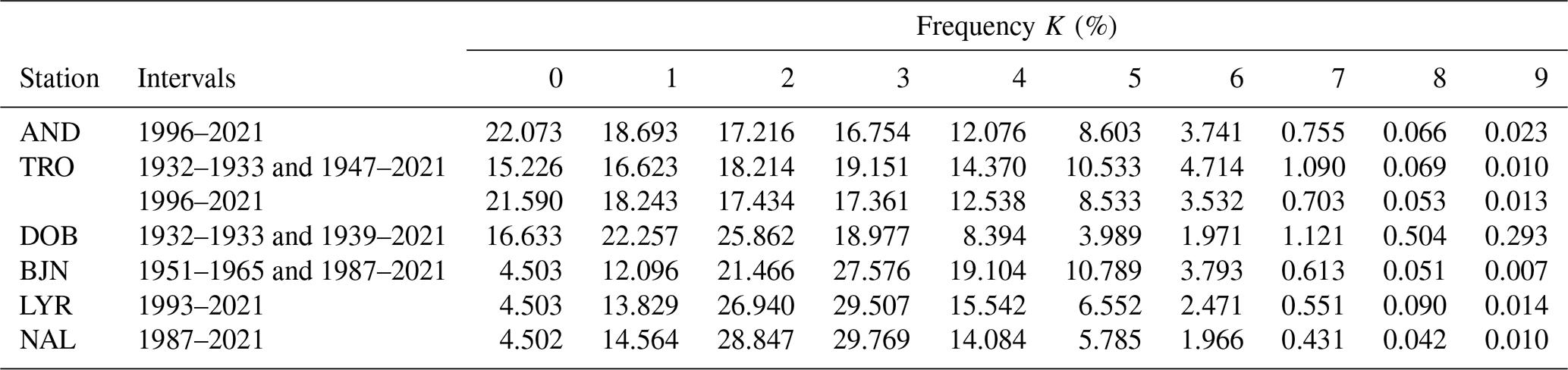
Frequency distributions for K should be log-normal-like with a peak frequency at K=2, following the standard K-index observatory in Niemegk (NGK). Also, values of K=2, 3 and 4 should account for >50 % of the cases. See Matzka et al. (2021) for further details on the ideal distribution. An appropriate K9 limit will result in well-fitting bins for each K value, meaning that the bins are a good fit for representing the K variation experienced at the station in question. Figure 3 shows distributions of K values for all six K-index stations in Norway: AND, TRO, DOB, BJN, LYR and NAL. All available K indices for each station are used in the corresponding histograms. The frequency distributions are also presented in Table A1.

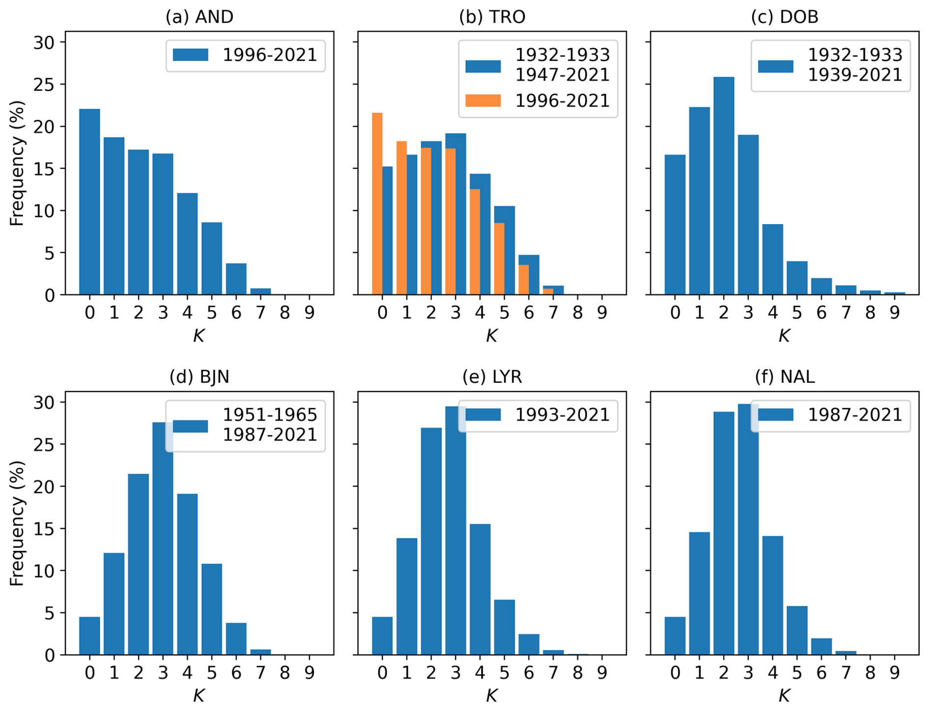
Figure 3 Histograms of K values for (a) AND, (b) TRO, (c) DOB, (d) BJN, (e) LYR and (f) NAL. The exact frequencies are shown in Table A1. The interval for each histogram is shown in each legend.

There are several points of interest concerning the distributions. We note that the distributions for BJN, LYR and NAL are similar in shape. All three distributions are well-tapered at both ends of the range for K and have a maximum frequency at K=3. This is close to the Niemegk distribution. It is also expected that the distribution for LYR will include slightly lower frequencies for low K values and higher frequencies for high K values than NAL. NAL is further into the polar cap than LYR, and it is reasonable to expect that LYR will therefore experience more geomagnetic variation due to the position closer to the auroral oval. This direct comparison is only possible because LYR and NAL share the same K9 limit (1800 nT). The DOB distribution is clearly log-normal-like with a peak frequency at K=2. However, the distribution includes a very high frequency of K=9 which requires further investigation.

The distribution for AND is drastically different from the remaining distributions. The same shape is seen for TRO in the same interval as AND, i.e., 1996–2021. The frequencies decrease with increasing K, the most frequent K value being K=0. Even though the K=0 frequency is large, we still have low, expected frequencies of K=9. The histogram for TRO improves when the whole interval is included. However, the skewed shape for TRO and AND cannot be ignored. The interval 1998–2021 includes only TGO-derived K indices. As discussed in Sect. 2.2.2, it is expected that the TGO method will assign lower values for K than HS. It is therefore of interest to, in more detail, inspect the overlapping period of K values for TRO and DOB during the transition between hand-scaling and the TGO method. Another option is that the shape is influenced by the included years and therefore the solar activity of the periods 1947–1996 and 1996–2021. This option will also be investigated.

In addition to the distribution features shown and discussed here, the distributions also exhibit expected seasonal and diurnal variation. That is, the frequencies of larger K values maximize during spring and fall, which is consistent with the well-known semi-annual geomagnetic variation (Lockwood et al., 2020, and references within). The frequencies of larger K values also maximize during nighttime (21:00–06:00 UT), consistent with substorm activity.

3.1 Distributions during the transition from hand-scaling to automatic methods

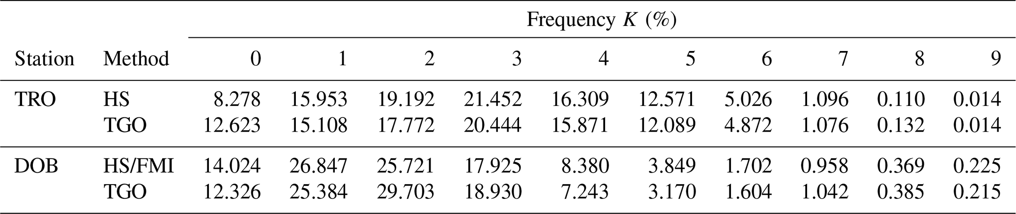
Figure 4 and Table A2 show distributions for K for TRO in the overlap interval 1988–1991 and for DOB in the overlap interval 1993–1998. K values derived by HS or FMI are shown in blue, and TGO-derived K values are shown in orange. For TRO, the shapes of the two distributions are similar. We note, as expected, that the TGO method includes a higher frequency of K=0. However, the distributions show no indication that the skewness for TRO and AND in Fig. 3 is a feature solely of the TGO method.

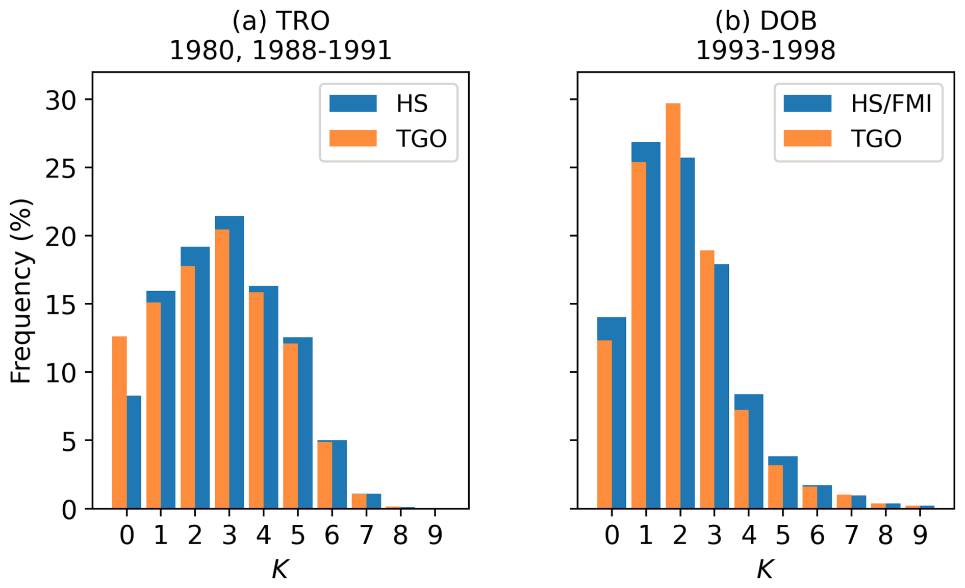
Figure 4 Distributions of K during overlaps in HS- or FMI-derived K and TGO-derived K for (a) TRO (1980, 1988–1991) and (b) DOB (1993–1998).

The general shapes of the distributions are also similar for DOB. However, we note somewhat larger differences between the two distributions. The differences are not systematic, but they are clearly larger for smaller K values (<4). It is not immediately clear why these differences occur, but a possible explanation is that, due to the low K9 limit of only 750 nT resulting in small bins of, e.g., 0–7.5 and 7.5–15 nT, the estimation of QDCs is of greater importance than that of TRO. Due to the small bins, there is a larger probability that a difference in QDCs of only a few nanotesla will move the range r into a different bin. Because of this, it is also possible that the deviations are a result of over-correction and under-correction owing to the TGO QDCs being averages over an entire solar cycle with the accompanying 10 nT uncertainty, which is bigger than the bin size. For both DOB and TRO, the presented distributions will be complemented in a later section by one-to-one comparisons of the K indices derived using the overlapping methods.

To better quantify the similarities of the distributions of hand-scaled and TGO-derived K indices, we have calculated the Pearson correlation coefficients for TRO and DOB. This yielded 0.978 and 0.893, respectively, showing good linear correlation between the distributions.

3.2 Distributions during maximum and minimum solar activity

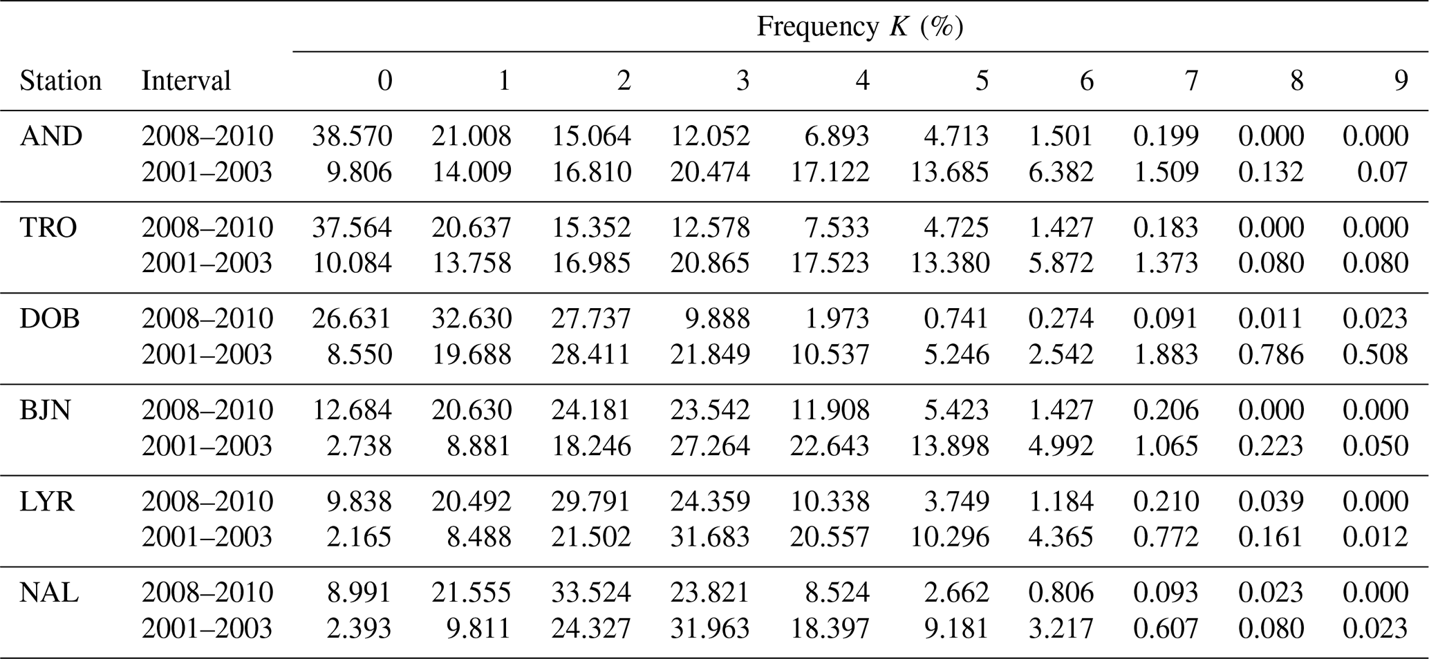
It is a well-known fact that geomagnetic activity peaks during the declining phase of the solar cycle and during solar maximum and that the activity is at its lowest during solar minimum. It is therefore of interest to investigate the distributions of K, especially for TRO and AND, but also for the other stations during solar minimum and maximum, to find out to what extent the distributions in Fig. 3 are influenced by the solar activity during the included years. Figure 5 shows histograms of K during a solar minimum (2008–2010) and during a solar maximum (2001–2003).

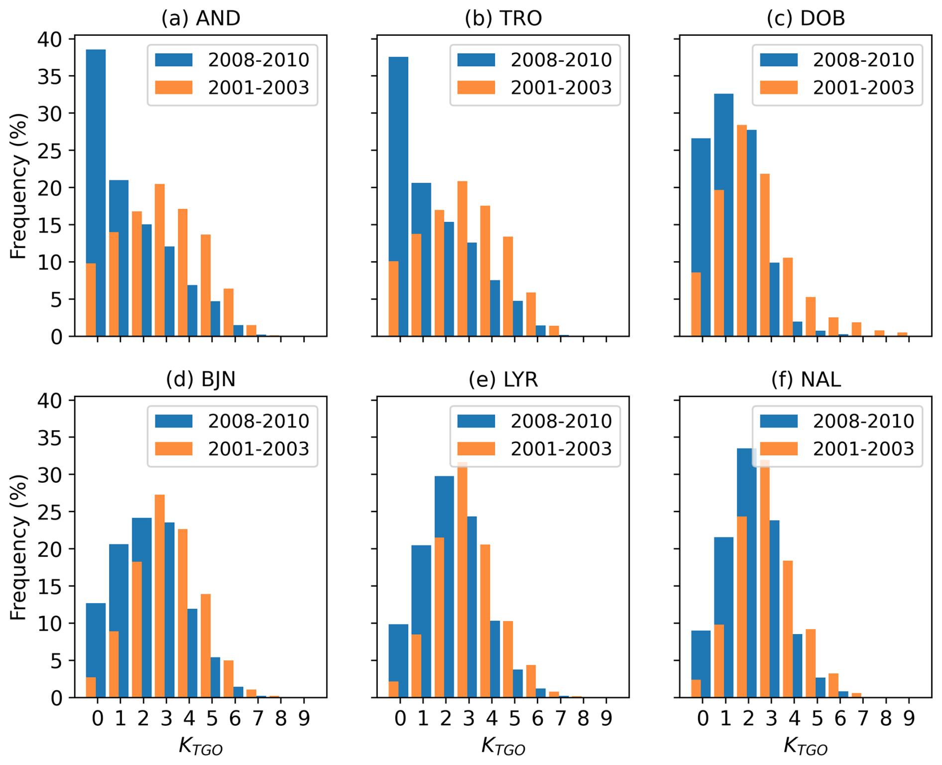
Figure 5 Distributions of TGO-derived K during a solar minimum (2008–2010) and during a declining phase (2001–2003) for (a) AND, (b) TRO, (c) DOB, (d) BJN, (e) LYR and (f) NAL.

It is of course expected that the shapes of the distributions for K will change with the degree of solar activity. We expect a shift towards higher K values during solar maximum and a shift towards lower K values during solar minimum. This is exactly what we see in Fig. 5 and Table A3 for BJN, LYR and NAL. The general shapes of the distributions do not change significantly, but we see the expected shift. Even though there are shifts in the distributions, the distributions for both low and high solar activity are well-tapered. We note zero frequencies for K=9 for all three stations, but this is not unreasonable for quiet years as the average frequency is about 0.01 % for the three stations.

We see the opposite in the distributions for TRO and AND. The frequencies during solar minimum of both K=9 and K=8 are zero, and the frequency of K=0 is almost 40 % for both stations. This skewed shape is not unique to this specific minimum but reoccurs during other minima for both AND and TRO in the TGO-derived K indices. The same skewed shape is also present during most minima in the series of HS-derived K indices for TRO, covering many solar cycles. It is therefore likely that the shapes of the skewed distributions for TRO and AND as seen in Fig. 3 are a feature of this strong solar activity dependence and not a result of some problem with the TGO method. This notion is also strengthened by considering the lower-than-usual levels of activity during solar cycle 24.

The distribution for DOB, shown in Fig. 5c, shows the expected shift towards higher K values during solar maximum. However, we see overly high frequencies of K=9 during solar maximum and also during the solar minimum. These relatively high K=9 frequencies in DOB might indicate that the K9 limit is set too low. An overly low limit will yield a higher-than-expected frequency of large K values. The possibility that the K9 limit is too low was discussed as early as 1943 during the first study of K indices calculated for the DOB observatory (Wasserfall, 1943), and the discussion is clearly still relevant.

Similarly, the zero frequencies of K=8 and 9 in AND and TRO might indicate that the K9 limit for AND and TRO is too high. This assumption is also strengthened by the fact that the K9 limit of 2000 nT is shared between AND, TRO and BJN. It is not unreasonable to assume that BJN experiences a higher level of geomagnetic disturbance. This is also evident from the distributions for BJN shown in both Figs. 3 and 5. The limit of 2000 nT represents the variation at BJN well. Therefore, it reasonable to assume that AND and TRO would benefit from a lower limit.

3.3 Lower or higher limits for K=9

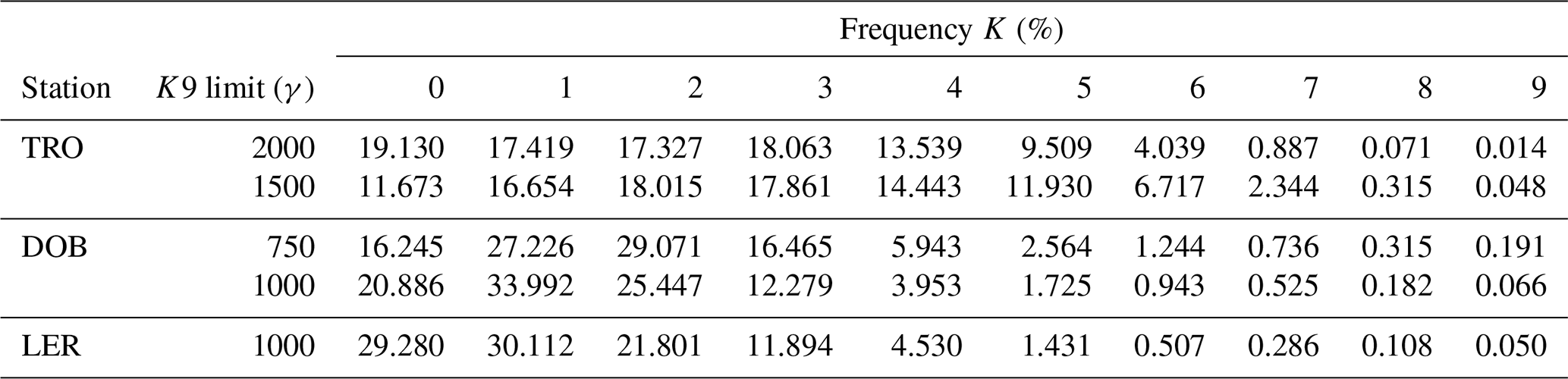
Figure 6 shows the results of an experiment where distributions for DOB and TRO are recalculated using K9 limits of 1500 and 1000 nT, respectively. This was done by rescaling digitally stored magnetograms with the new lower limits, using the TGO method. In Fig. 6a it is clear that the distribution shape for TRO is very different, with peak frequencies at K=2 and K=3. The new limit of 1500 nT has not resulted in an overly high frequency of K=9, and the frequency of K=0 is reduced. This clearly indicates that the new limit is a better fit for the variation experienced at TRO. The fact that the change in the distribution is most significant for K=0 means that this adjustment would not negatively affect the reasonable distribution shape for the entire series shown in Fig. 3.

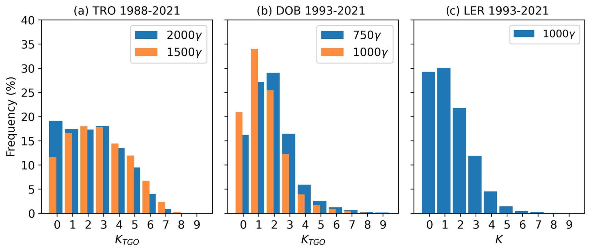
Figure 6 Histogram of K values for (a) TRO, K9 limit = 2000γ (original) and TRO, K9 limit = 1500γ (adjusted). (b) DOB, K9 limit = 750γ (original) and K9 limit = 1000γ (adjusted). (c) LER, K9 limit = 1000γ (original).

It is difficult to conclude whether the new limit for DOB is a better fit than the original limit. The frequency of K=9 is slightly reduced, and the frequency of K=0 increases. However, this increase in K=0 is undesirable compared to the Niemegk distribution (Table 2). In addition, the frequency of K=9 is still higher than we would expect. For comparison, Fig. 6c shows the distribution of K from 1993 to 2021 from Lerwick (LER), Shetland (retrieved from BGS Geomagnetism at http://www.geomag.bgs.ac.uk/data_service/data/magnetic_indices/k_indices.html, last access: 9 October 2024). The K9 limit for LER is 1000γ, and LER is south of DOB by only a few degrees in geomagnetic latitude. The distribution for LER is skewed towards low K values. However, the frequency of K=9 is similar to that for DOB, with a K9 limit of 1000 nT. We cannot say that the K9 limit in DOB is too small, as the distribution does not necessarily improve with a higher limit. This is also indicated in Fig. 5, where it is clear that the distribution shape is robust to changes in solar activity and therefore to changes in geomagnetic activity if we do not include the high K9 frequency.

It is shown that the 1500γ limit is a better fit for the variation experienced at the TRO station. However, the limit cannot be replaced. For the sake of continuity with the manually derived K values and preservation of the historic assignment of the limit, the original K9 limit of 2000γ must be used (this also applies to the K9 limit for DOB). Nevertheless, the knowledge is valuable as it explains the unexpected distribution shape with the high density of K=0, together with the sensitivity to which years and therefore which part of the solar cycle is used when calculating the K distribution. It also means that K values from TRO and, say, DOB do not necessarily correspond to the same level of relative variation. In turn this means that the K values cannot be used as a tool for directly comparing variation between the stations. Finally, an ill-fitting K scale will not affect the validity of the K series as measures of the time variation of geomagnetic activity at each observatory. Therefore, the derived index ak and yearly Ak are still good measures of the time variation at each observatory.

4 Comparisons of K derivation methods

During the overlap periods between old and new series for TRO and DOB, K indices are derived by various methods. For DOB the overlap period (1993–1998) includes three methods, which include overlaps between K indices derived by the TGO method and both HS and the FMI method. For TRO the overlap period (1988–1998) also includes three methods, which are between K indices derived by the TGO method, an early version of the TGO method (the TGOe method) and hand-scaling. A second overlap exists between HS-derived K indices and K indices derived by the TGO method applied to digitized magnetograms for the year 1980. Comparisons of the methods during overlapping periods are discussed in Sects. 4.1 and 4.2.

We have seen that the TGO method provides a good match with the HS- and FMI-derived K values in the old and new series for TRO and DOB (Fig. 4). However, it is also interesting to compare the performance of the TGO method against an acknowledged method. For this we chose the FMI method (Sucksdorff et al., 1991). The FMI method has been applied to the same data as the TGO method for this study. A comparison of the resulting K indices is presented in Sect. 4.4.

4.1 Comparing K derivation methods during overlap periods: DOB

For DOB, the TGO method and HS derivation overlap in the interval 1993–1994. The FMI method and the TGO method overlap during 1995–1998. Figure 7 shows the densities of all possible (a) (K_HS,K_TGO) pairs and (b) (K_FMI,K_TGO) pairs during the overlap periods. For the K indices derived by the FMI method, the yearbook for 1995 (Institute of Solid Earth Physics, Geomagnetism, 1997) notes that the K indices for this year are primarily calculated by the FMI method but that some indices are hand-scaled. The same is noted in the yearbooks from 1996 (Institute of Solid Earth Physics, Geomagnetism, 1998), 1997 (Institute of Solid Earth Physics, Geomagnetism, 1999) and 1998 (Institute of Solid Earth Physics, Geomagnetism, 2000).

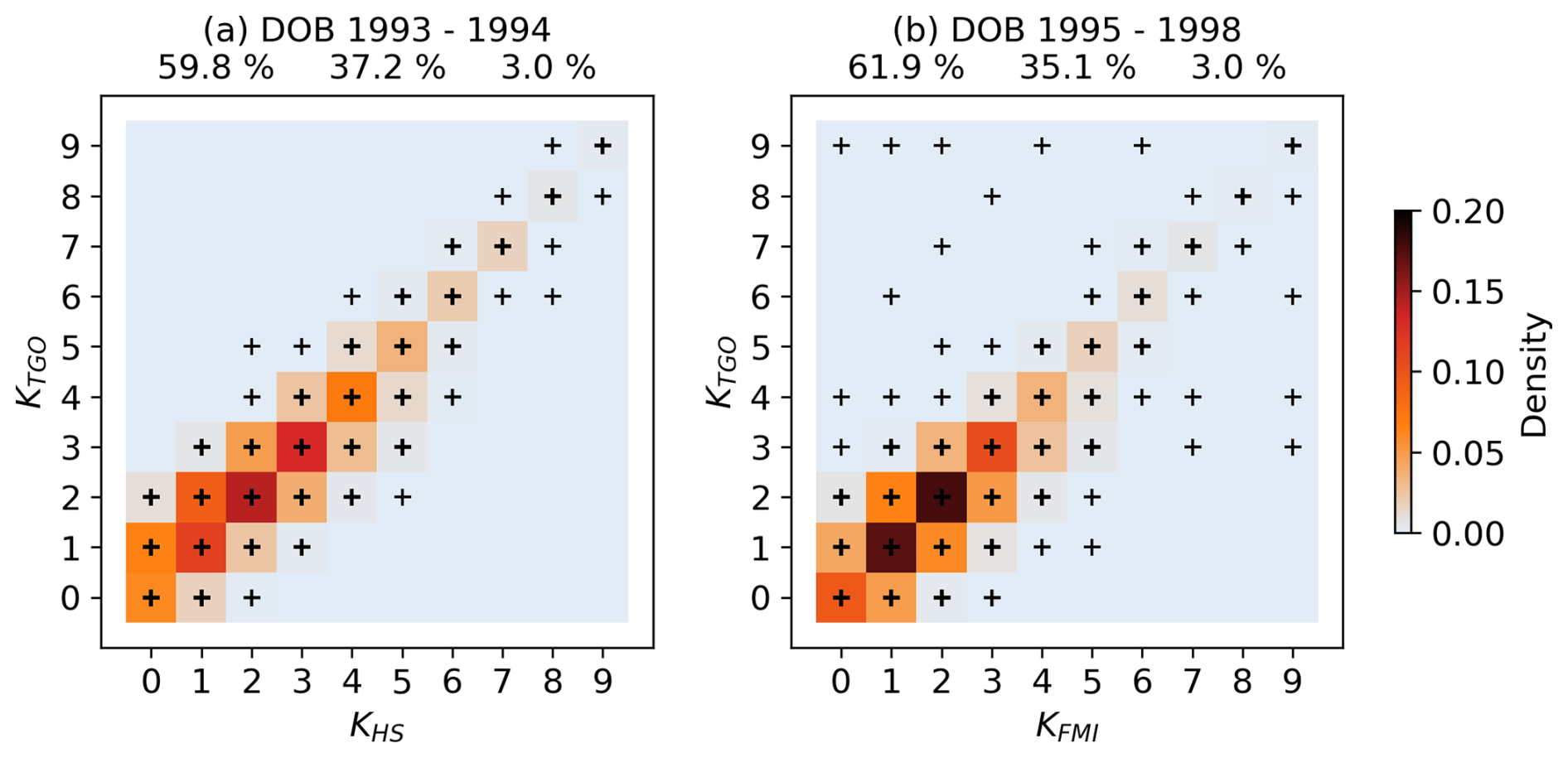
Figure 7 Comparison of (a) HS-derived K indices and TGO-derived K indices and (b) K indices derived using the FMI method and TGO-derived K indices for DOB. The black crosses denote every pair with a density that is nonzero. Unmarked locations have a density of zero. The frequencies of perfect matches, deviations by 1 unit and deviations by more than 1 unit are shown above each plot.

In general, the agreement between the methods in both comparisons is good, with clear abundances of perfect matches. However, about one-third of the pairs deviate by 1 unit, and only 3 % of the pairs deviate by 2 or more units in both comparisons. In Fig. 7b there is a large count of outliers. The most severe disagreement is seen in the upper-left corner, where K_TGO=9 is paired with $K_{\text{FMI}}=\mathit{\{}\mathrm{0},\mathrm{1},\mathrm{2}\mathit{\}}$. However, all three points correspond to the same day, i.e., 25 September 1998. On this date the digital DOB magnetogram clearly exhibits stormy conditions. The same conditions are visible in the digital TRO magnetogram. During this overlap period the DOB station operated two digital variometer systems (Institute of Solid Earth Physics, Geomagnetism, 2000). The magnetograms that are stored digitally today at TGO are results from the primary variometer system. The published K indices are calculated from magnetograms from the secondary variometer system. It is therefore plausible that the $K_{\text{FMI}}=\mathit{\{}\mathrm{0},\mathrm{1},\mathrm{2}\mathit{\}}$ values, which are recorded in the DOB 1998 Yearbook (Institute of Solid Earth Physics, Geomagnetism, 2000), are erroneous, possibly due to a fault in the secondary variometer system or a human error.

The outliers where K_FMI=9 and K_TGO=4 in Fig. 7b, which occurred on 4 May 1998, can be explained by looking at the stored digital magnetogram from the same day. As explained in Sect. 2.2.2, the TGO method will calculate K based on any interval containing data, no matter the size of the potential data gap. This can lead to erroneously small K values. This is the case for 4 May 1998. The H component for this date is plotted in Fig. 8. A large gap in the data has affected the second (03:00–06:00 UT) and third (06:00–09:00 UT) intervals. In the second interval the variation is larger than the K9 limit of 750 nT, and the TGO method therefore correctly assigns a K value of 9 despite the missing data. In the third interval, the TGO method assigns a K value of 4 based on only the 25 min of data in the interval, even though the value could be larger based on the size of the data gap. However, the FMI-derived K value, based on the secondary variometer system that likely did not include this data gap, assigns K=9. It is therefore likely that K_TGO=4 is wrong and a result of the TGO method allowing any data gap. This is also seen in other cases where the TGO method assigns a significantly lower value than both the FMI method and HS derivation.

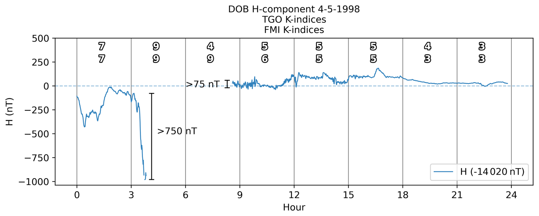
Figure 8 H component for DOB on 4 May 1998. The top row of indices is derived using the TGO method, and the second row is derived using the FMI method.

The allowance of any size data gap leads us to expect a tendency in which the TGO method assigns lower values for K than HS-derived K. However, the opposite tendency can be seen in Fig. 7a, especially for low K values. This is possibly a result of the correction values being averaged over a solar cycle. This leads to over-correction or under-correction of the magnetograms, especially during solar minima or maxima. Over-correction will introduce false variation, whereas under-correction will fail to remove all non-K variation. Either way, the variation in the corrected magnetogram will be slightly larger than what should be expected. This has possibly resulted in the TGO method assigning larger K values than the HS K values, especially for the smaller K values, where the QDCs have a greater influence on the range r and therefore the assigned K. It is possible that it is necessary to implement less simple QDCs that account for solar cycle variation of the Sq current system and therefore the quiet-day variation. Another explanation for the shift towards a larger K_TGO for low K values is an issue with the rigid QDCs, where it is possible that shifts in time can lead to larger K values. This is explored in Sect. 4.4.3.

The deviations of 1 unit are symmetric between the FMI method and the TGO method (Fig. 7b). The DOB 1995 Yearbook (Institute of Solid Earth Physics, Geomagnetism, 1997) notes that the agreement between K_HS and K_FMI is generally good, with 75 % perfect matches. It also notes that, for the deviations of 1 unit, K_FMI>K_HS in 15 % of the cases and K_FMI<K_HS in 10 % of the cases. The comparison is performed for only a few months.

4.2 Comparing K derivation methods during overlap periods: TRO

For TRO, the TGO method and hand-scaling overlap from 1988 to 1991. From 1992 to 1998, K values based on the TGO and TGOe methods are available. The difference between the two is that the TGOe method uses correction values derived from the quietest days in every month in every year. In 1980 there is an overlap between hand-scaled values and the values based on the TGO method applied to the same magnetograms, which exist in digitized form. Figure 9 shows the densities of all possible (a) (K_HS,K_TGO) pairs, (b) (K_TGOe,K_TGO) pairs and (c) (K_HS,K_TGO) pairs during the overlap periods.

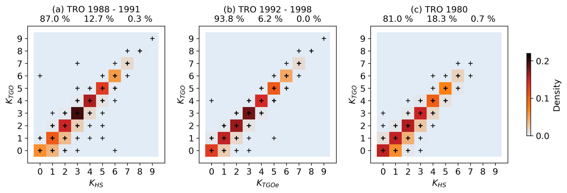
Figure 9 Comparison of (a) HS-derived K indices and TGO-derived K indices, (b) K indices derived by the TGO method and TGO-derived K indices and (c) HS-derived K indices and K indices derived by applying the TGO method to digitized magnetograms for TRO. The black crosses denote every pair with a density that is nonzero. Unmarked locations have a density of zero. The frequencies of perfect matches, deviations by 1 unit and deviations by more than 1 unit are shown above each plot.

From Fig. 9a and b it is clear that the agreement between the K indices derived by the two methods, during their overlap periods, is good. There is also a low number of outliers in all the comparisons, and the distributions are narrow, including less than 1 % of outliers of more than 1 unit. As is the case for DOB, the outliers in (K_HS,K_TGO) can also be explained by (1) likely wrong K values reported in the yearbook or (2) large data gaps leading the TGO method to give overly low K values.

All three distributions are asymmetric, showing clearly that for TRO the TGO method is prone to assigning lower values for K than K_HS, as expected when data gaps are large in the TGO method. The signatures of over-correction and under-correction that were visible in the DOB comparison in Fig. 7a are not visible for TRO in Fig. 9a. It is likely that over-correction and under-correction still occur, but we expect a significantly lower frequency due to the lower amplitudes of the QDC (Fig. 2) and the larger bins for K, which makes it less likely that under-correction and over-correction will affect the assignment of K.

In Fig. 9c, where the TGO method is applied to the digitized magnetograms from 1980, the asymmetry is stronger towards lower K_TGO. This is possibly a feature of the digitization of the magnetograms. The digitization was performed by human hand, and it is therefore likely that a bias is introduced.

The match between K_TGO and K_TGOe, shown in Fig. 9b, is almost perfect, with a percentage of 93.8 % of perfect matches and virtually no deviations above 1 unit. This is reasonable as the methods are identical except for the correction values. The asymmetry toward K_TGOe>K_TGO indicates a systematic difference between K_TGOe and K_TGO, likely due to the different correction values and under-correction and over-correction. The almost perfect match between indices derived by the TGO and TGOe methods clearly shows that there is no harm in using averaged QDCs when computing the K indices for TRO.

4.3 Summary of the compared methods

Generally, all five comparisons presented in Figs. 7 and 9 show good agreement. It is also evident that the agreements are better for TRO than for DOB. However, it is important to recall the K distributions and the overly high K9 limit for TRO. This results in fewer chances of errors as a larger portion of the variation is easily placed in the K=0 bin. As the bins for K=8 and K=9 are less frequently used, there are smaller chances of errors. We can see this in Fig. 9c. In 1980, neither K=8 and K=9 is used. This means that the variation is only between eight bins.

It is also important to note that it is not clear whether these overlapping years are representative of all years. The overlaps are short and should ideally cover at least a solar cycle to be representative. It is therefore not possible to say whether these comparisons produce results that are worse or better than for an average year.

In all the comparisons in Figs. 7a and 9a, we see cases where K_HS>K_TGO for all values of K. Apart from this tendency being a result of the TGO method assigning lower K values to intervals with large data gaps, this is also likely a result of the transition from K determination based on analog magnetograms to applying the TGO method to 1 min resolution data. Sampling in a digital system and computing 1 min resolution data act as a low-pass filter. The magnitudes of disturbances in the digital 1 min data will therefore be slightly smaller than the magnitudes of recordings in the analog systems.

The diagonal where $K_{\text{HS}}=K_{\text{TGO}}+\mathrm{1}$ is slightly denser for DOB than for TRO: it is possible that this is a feature of the H>D assumption that is applied in the TGO method. It is possible that the assumptions are not valid for DOB since DOB is a subauroral station. In cases where the variation in D is greater than that of H, K(D), which is calculated when hand-scaling, will obviously be larger than K(H), which is the only value calculated using the TGO method.

When evaluating K derivation methods, IAGA-accepted methods achieved at least 69.9 % agreement with HS-derived K (Matzka et al., 2021) and less than 2 % deviations of more than 1 unit. Following these criteria, the TGO method is clearly an acceptable method when used at TRO. For DOB the two criteria are not met for the TGO method. However, given the short overlaps and the fact that we cannot say whether the comparisons presented in this paper are representative of an average year, it is possible that the criteria could be met. It is also highly likely that adjusting the method, e.g., by including a maximum data gap length, would increase the accuracy.

To summarize, we can confidently say that the TGO-derived K values are a valid continuation of the HS-derived K values for TRO. For DOB the same conclusion cannot be drawn confidently.

4.4 The TGO and FMI methods

The FMI method has only been used in Norway in the short interval 1995–1998 at DOB. For this study, the FMI method was applied to the digital TGO data. This was done, as mentioned, to compare the TGO method against an acknowledged K derivation method, which the FMI method is. In this section we compare the FMI method to the TGO method, with and without applying the assumption H>D. We also investigate a number of specific days and magnetograms.

Figure 10 shows comparisons of corresponding pairs of (K_FMI,K_TGO) for all six Norwegian K-index stations. The percentages above each plot are the percentages of perfect matches between K_FMI and K_TGO, deviations of 1 unit and deviations of >1 unit. Generally, it is clear that the agreement between the K indices derived by the TGO method and the FMI method is good. For DOB the agreement is slightly worse than for the rest.

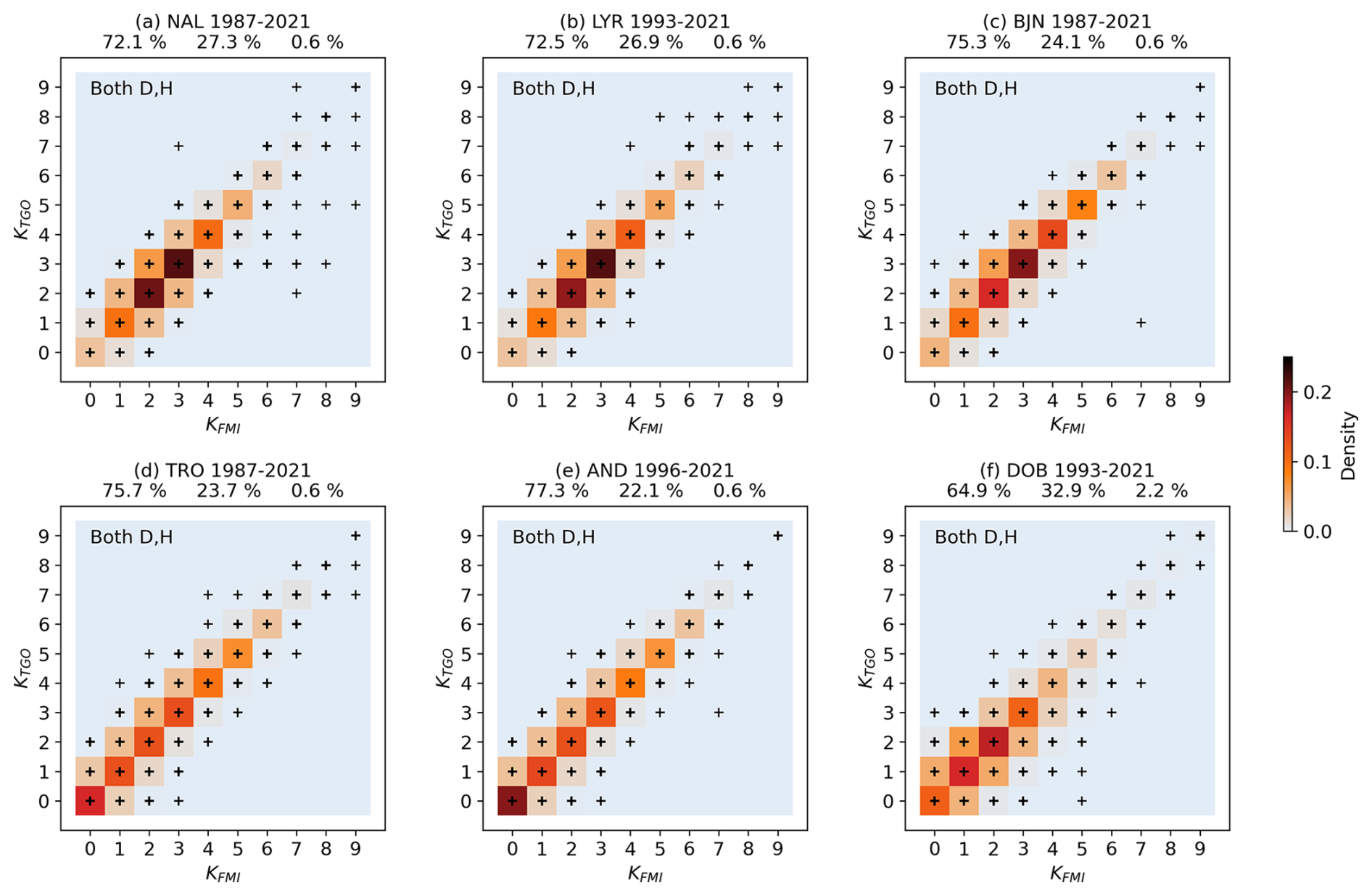
Figure 10 Comparison of (K_FMI,K_TGO) pairs for (a) NAL, (b) LYR, (c) BJN, (d) TRO, (e) AND and (f) DOB. The colors give the density of each (K_FMI,K_TGO) pair occurring in the interval given in the title. The black crosses show every pair that has occurred. The percentages over each plot are the percentages of perfect matches between K_FMI and K_TGO, deviations of 1 unit and deviations of >1 unit.

The distributions for BJN, TRO and AND are clearly asymmetric, with a shift towards deviations of 1 unit where K_TGO>K_FMI. It is not obvious why this is the case. However, Sucksdorff et al. (1991) note that the FMI method is sensitive to disturbances during the night when estimating QDCs. They show that a fitted QDC often follows the disturbances during the night, leading to an erroneous QDC that also includes K variation. For BJN, TRO and AND there are usually disturbances during the night, since they are all located in the auroral zone and the auroral electrojet is observed practically every night. These erroneous QDCs can result in smaller K values since K variation is subtracted from the QDC. This can explain the strong asymmetry and especially why we see the same asymmetry for both large and small K, which is different for the under-correction and over-correction in the TGO method, which is only visible for lower K values as observed in Fig. 7a.

4.4.1 The H>D assumption

To investigate the significance of the H>D assumption, we first calculate FMI K indices based on both D and H. Then, the FMI method is also applied to the H component only by feeding the algorithm with H values as input for both H and D, i.e., by setting D=H. The two resulting sets of K indices are compared to TGO-derived K indices in Figs. 10 and 11.

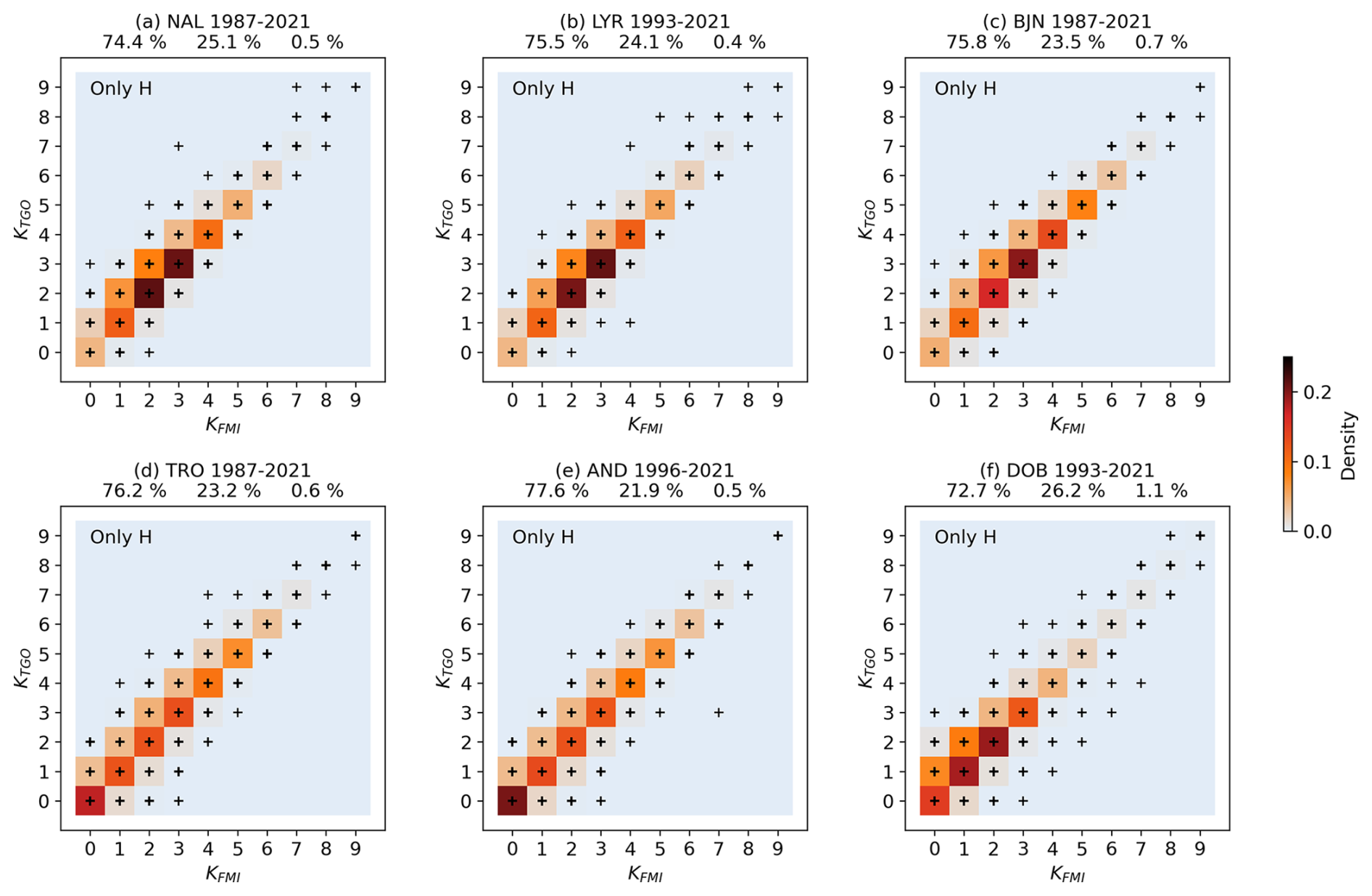
Figure 11 As in Fig. 10: here the assumption H>D is used and the FMI method is used with H only.

First, for BJN, AND and TRO, only small differences in the distributions and frequencies of the matches and deviations can be seen. This implies that the assumption H>D is valid at these locations. This is expected because these stations are in the auroral zone. For NAL and LYR there is a slightly higher increase in the percentage of perfect matches than when the assumption is not applied. We also note that the distributions are clearly asymmetric. The deviations towards a higher K_FMI have almost disappeared when compared to the distributions shown in Fig. 10. This means that these deviations were caused by K indices based on D where D>H. Further, this implies that, for these cases, the H>D assumption is broken.

The same can be seen for DOB. The agreement improves drastically when the FMI method is applied with D=H. As for NAL and LYR, the deviations of 1 unit where K_FMI>K_TGO mostly disappear compared to the distribution shown in Fig. 10. Again, this implies that the deviations are the result of K based on D where D>H and that the assumption of H>D is invalid.

4.4.2 Individual case comparisons between the TGO and FMI methods

Figure 12 shows three sets of 3 d intervals of magnetometer H and D components, K values derived by both the FMI and TGO methods as well as the range of the TGO method's quiet curves and the QDCs fitted by the FMI method. The ticks on the x axis show the start and stop hours of each interval. The QDCs returned by the FMI method have been shifted by subtracting their means for easier comparison with the magnitudes of the TGO QDCs. Figure 12a shows TRO data from the center date 10 November 2022. This date is remarkably quiet. Under these conditions we see that both the FMI method and the TGO method assign only K=0 and that their QDCs are highly comparable. Figure 12b shows another quiet, but somewhat more disturbed, day for DOB (10 November 2021). For this case the K values assigned by the FMI method and the TGO method are also identical, except for the fourth interval, and the QDCs are practically comparable.

Next, Fig. 12c shows a magnetogram from TRO. For the three dates covered, i.e., 4 October 2022, 5 October 2022 and 6 October 2022, there are clear disturbances at night. As mentioned above, a known limitation of the FMI method is the sensitivity to disturbances at night when fitting the QDC. This is clearly visible in the figure; the fitted QDC is clearly influenced by the disturbances in both shape and amplitude. For the intervals 09:00–12:00 UT and 12:00–15:00 UT, the assigned K_FMI values are smaller than K_TGO by 1 unit, likely due to the overly large QDC that has been subtracted. Disturbances during several successive nights are highly common at auroral latitudes, and this is not unique to the presented case.

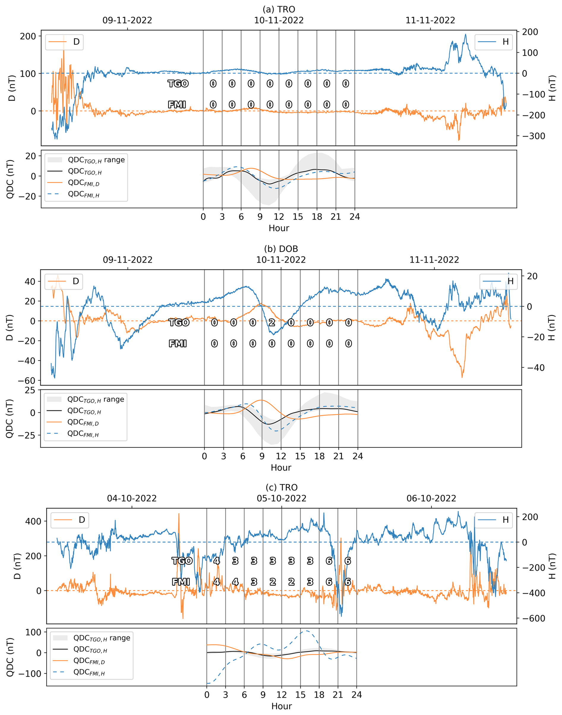
Figure 12 Magnetogram H and D components, K derived by the TGO and FMI methods, TGO method correction values and FMI QDCs for (a) TRO 10-11-2022, (b) DOB 10-11-2022 and (c) TRO 05-10-2022.

4.4.3 Differences in the K variation

Figure 13 shows magnetogram H components, QDC_FMI and QDC_TGO, and the calculated K variation for (a) DOB 10-11-2022 and (b) TRO 05-10-2022. These dates show two important cases when calculating the K variation.

Figure 13 K variation based on the QDC from the FMI method and the TGO method DOB 10-11-2022 (a, as in Fig. 12b) and TRO 05-10-22 (b, as in Fig. 12c).

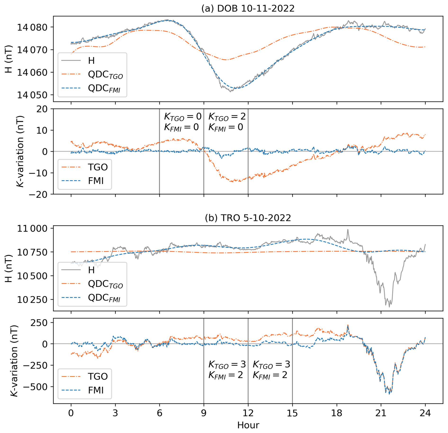
Figure 13a shows a possible problem when dealing with rigid QDCs: 10 November 2022 is clearly a quiet day for DOB when looking at the magnetogram. However, due to a phase shift in the quiet-day variation on this date, there is a shift between the H component and QDC_TGO leading to K=2 in the 09:00–12:00 UT interval. This example is a “worst case”, and shifts this severe, leading to an error of more than 1 unit, are rare. However, errors of 1 unit occur regularly. This error is likely a contributing factor in the asymmetry towards larger K_TGO for lower K values in DOB, as seen clearly in Fig. 7a, and why the agreement between the FMI and TGO methods is worse for DOB than for the remaining Norwegian stations. Shifts in the quiet-day variation in TRO also occur. However, due to the larger bins for the low K values for TRO, the assignment of K is rarely affected.

Figure 13b shows the K variation where QDC_FMI is affected by disturbances during the night. The magnetograms of the previous and next days are shown in Fig. 12b. Owing to the large magnitude of QDC_FMI, the K variation differs by up to 120 nT. For the intervals 09:00–12:00 UT and 12:00–15:00 UT, the FMI method assigns K=2, which is 1 unit lower than the TGO method. This effect is likely a contributing factor in the portion of deviations where $K_{\text{TGO}}=K_{\text{FMI}}+\mathrm{1}$ in Fig. 10.

4.4.4 Summary of the comparison of the TGO and FMI methods

We have seen that, for all the Norwegian K-index stations except DOB, the agreement with the FMI method is good and the expectation of at least 70 % correlation is met. For all of the stations except DOB and BJN, the deviations above 1 unit are less than 2 %. For BJN the percentage is slightly higher, but due to its extremely remote location this observatory is more prone to significant data gaps which have likely affected K_FMI. For DOB, LYR and NAL, we have seen that the assumption that H>D is broken often enough to yield visible differences in the comparisons when the FMI method is applied with and without the assumption.

Several causes of differences between K_TGO and K_FMI are summarized as follows. Disturbances during the night can result in large QDC_FMI and therefore K_FMI<K_TGO. Both shifts in the quiet-day variation with respect to time and over-correction and under-correction can result in K_FMI<K_TGO. If the assumption H>D is broken and the variation in the D component is larger, K_FMI>K_TGO.

5 The Ak time series

Figure 14 shows the complete series of the yearly averaged Ak index for BJN, DOB and TRO. Note that, for the curves to be more easily distinguishable, BJN and TRO are plotted with offsets of 15 and 7.5 nT, respectively. The solid lines show the series obtained from the yearbooks and IAGA bulletins. For DOB and TRO these series include a transition period from HS derivation of K to automatic derivation, as was discussed earlier. The series for DOB includes a short interval where the FMI method was used, from 1995 to 1998. The dashed lines show the series resulting from the TGO method. The points for BJN and TRO in 1980 denote an Ak resulting from applying the TGO method to magnetograms that were digitized for a study by Walker et al. (1997). The yearly sunspot number (retrieved from WDC-SILSO Sunspot Number, Royal Observatory of Belgium, Brussels https://www.sidc.be/silso/datafiles, last access: 5 May 2025) is shown as grey shading.

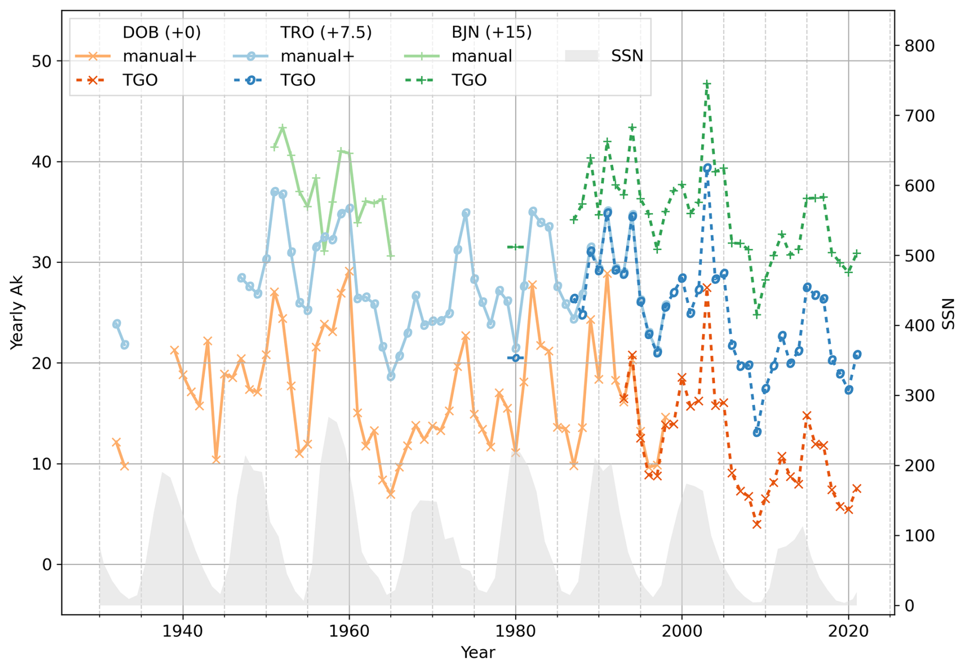
Figure 14 Yearly Ak index from the stations in DOB (reds and oranges), in TRO (blues and purples) and in BJN (greens). The dashed lines show the automatically derived values. The solid lines show manually derived values. The “+” in “manual+” denotes short transition periods from hand-scaling to derivation by the TGO method.

The series from all three observatories generally express the same variation with time. All three series show expected local maxima during the declining phases of the solar cycle and smaller local minima in the beginning of solar maxima. The yearly Ak shows a clear global minimum in 2009 for all three stations, which is the quietest year on record. The global maximum is reached in 2003 for TRO and BJN and in 1991 for DOB. The global minimum in 2009 and the global maximum in 2003 are shared with the observatory in Sodankylä (SOD), Finland (Nevanlinna et al., 2011), which is closer to TRO than DOB in magnetic latitude.

The shape of the curve at BJN strongly deviates from the shape of the curves at TRO and DOB in 1958. The 1958 yearbook (Norwegian Institute for Cosmic Physics, 1960) makes no mention of anomalies at the BJN observatory during the year 1958. Upon closer inspection of the monthly averaged Ak values for TRO and BJN, it was revealed that there is a clear and systematic deviation between the two stations only from January 1958 to June 1959. It is likely that this systematic deviation is of a nonphysical origin. The scale values used at TRO are unchanged during this period, while the scale values for BJN are changed by only 0.1 nT (Norwegian Institute for Cosmic Physics, 1959, 1960, 1961). It is possible that the deviation is caused by human errors or that there were some differences in operations or routines at BJN during the IGY (1957–1958). We have not been able to identify any written references describing this issue.

The agreement of the overlapping series in TRO and DOB is generally good. The overlap in TRO is seemingly an almost perfect match, except for a small difference in the first year, 1988. The differences between the overlapping series are larger in DOB, with a maximum difference in 1997. However, for both stations it is clear that yearly Ak is an excellent measure of the long-term variation and that the curves resulting from HS-derived K and TGO-derived K agree well.

Power spectra of daily Ak

Power spectra of daily Ak should exhibit several well-known spectral lines corresponding to solar and geomagnetic effects (Matzka et al., 2021). Figure 15a and b show power spectra of daily Ak for TRO and DOB computed through fast Fourier transforms (FFTs) of the complete series, the red noise power spectrum and the 95 % confidence level. Both series only include a small number of gaps in the data. These gaps have been filled with zeros. The complete series are constructed by simply joining the series of HS- and FMI-derived Ak with the TGO-derived Ak. The series are joined in 1998 under the assumption that the series of TGO-derived K is a valid continuation of the series of HS- and FMI-derived K. As seen in Fig. 14, and as elaborated on in the previous sections, this assumption is valid. The power spectra for TRO and DOB are similar. The slight differences in positioning of the spectral lines can be attributed to the fact that the series for DOB is 8 years longer than the series for TRO, which corresponds to almost an entire solar cycle.

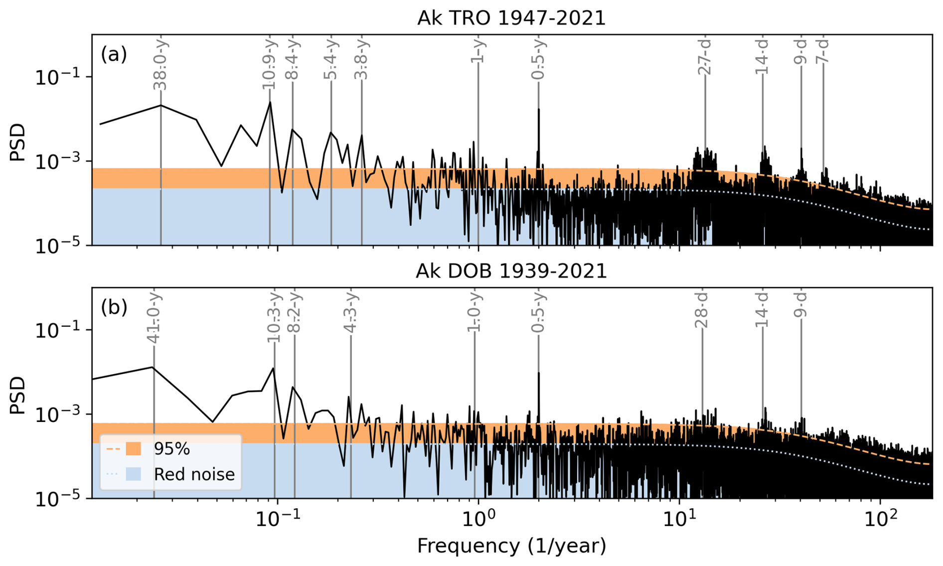
Figure 15 Power spectrum for the daily Ak series from (a) TRO 1947–2021 and (b) DOB 1939–2021. The blue shade (dotted outline) shows the red noise power spectrum, and the orange shade (dashed outline) shows the red noise power spectrum 95 % confidence level.

As expected, both spectra exhibit well-known spectral lines corresponding to the solar cycle at 10.3 and 10.9 years and the dual-peak structure of solar maxima at 5.4, 4.3 and 3.8 years. Both spectra also include strong lines at 8, 8.4 and 8.2 years. It is possible that these lines correspond to the distance from the secondary peak of one solar cycle to the primary peak of the next cycle. In addition, both spectra include strong spectral lines at 0.5 years corresponding to the semi-annual geomagnetic variation (Lockwood et al., 2020). Both spectra also include spectral lines corresponding to Earth's orbit, 1.0 years, and the solar rotation at 27 and 28 d. Furthermore, both spectra exhibit lines at harmonics of the solar rotation frequency, i.e., at 14 and 9 d for DOB and TRO and at 7 d for TRO. This is consistent with the periodogram shown by Matzka et al. (2021). The peak frequency around each harmonic is rounded to the closest day to match the time resolution in our series, which is 1 d. The spectral lines at the first and second harmonics are believed to be caused by coronal holes separated by 180 or 120° in solar longitude (Temmer et al., 2007). The spectra for TRO include a spectral line around 7 d that corresponds to the fourth harmonic of the solar rotation frequency. It is possible that these lines are due to four coronal holes separated by 90° in solar longitude. Finally, both spectra show low-frequency components for both TRO and DOB at 38.0 and 41.0 years, matching the low-frequency components in similar spectra for daily Ak and global daily aa (Nevanlinna et al., 2011).

The spectrum for DOB is clearly noisier than the spectrum for TRO; this is especially clear towards the higher-frequency part of the spectrum. There are two possible explanations for this noisiness. First, DOB is located at a significantly lower geomagnetic latitude than TRO. It is therefore reasonable that solar–terrestrial interaction effects are more clearly visible in TRO than in DOB. Second, it is likely that DOB data, especially up to the 1950s, are influenced by various environmental factors that possibly influenced the recordings. These environmental factors are discussed in detail in, e.g., Wasserfall (1953) and Gjellestad et al. (1957). To check whether these environmental factors have had a significant influence on the spectrum for DOB, the spectra were calculated in different intervals in time, excluding data up to 1952 and excluding all manual scaling. However, the noise level did not change noticeably.

6 Discussion and conclusions

In this paper we have reviewed the K values generated for various locations in Norway during the last century and described where these have been published and how they have been calculated. We have also described the effort of digitizing all the identified K indices. For the longest time series at DOB and TRO, manual scaling of K ended at about the same time as the transition from classic, analog variometers to digital flux-gate magnetometers. Since these two observatories have been run by different institutes during most of their lifetimes and the documentation is limited, we have not been able to identify the practices of different scalers, and we can only assume that they have followed the procedures as recommended in the literature (e.g., Mayaud, 1980). Several different approaches have been taken in the digital era for automatic determination of K, and limited periods of time contain overlaps between hand-scaling and automatic schemes. We have investigated these overlap periods in order to determine whether the time series may be considered continuous across the transition.

Investigating the frequency distributions of different K values for the different stations, a few peculiarities were uncovered. In particular, the auroral stations on the mainland (TRO and AND) show too many low K values with the maximum at K=0 and too few high K values as compared to the “ideal” distribution (Table 4); i.e., the distributions are skewed towards low values. Furthermore, the frequency of K=9 is too high at Dombås. The skewness at TRO and AND was carefully investigated, where frequency distributions were examined for periods of high and low solar activity and for the possibility of the scaling methodology introducing problems, but neither could be the reason. Comparing neighboring observatories, we realized that the K=9 threshold of 2000 nT chosen a long time ago could be the reason for the skewness, and we performed a test on the digitally available data and reduced the threshold to 1500 nT (same as for the Sodankylä magnetic observatory). This improved the shape of the frequency distribution to our satisfaction, leading us to conclude that the choice of a threshold of 2000 nT is not justifiable. However, the threshold was set a long time ago, when no statistical basis existed for its determination. Since the majority of the data still only exist as analog records and changing the threshold would require hand-scaling of more than 50 years worth of data, together with the fact that the index has been used in previous studies, the threshold should be kept as is. This is no problem in itself, since it does not affect the time series analysis of the index itself or its use in the analysis of other local time series. Furthermore, since the K indices from TRO or AND are not combined with other stations to derive regional or global indices, no problems can be seen in that respect either. One should, though, show caution when comparing the K indices from these stations with those from other stations or at least be aware of the skewness in the distributions. Considering that K already has a questionable value (e.g., Menvielle et al., 2011) at high latitudes, since it does not necessarily reflect the magnetic energy density of the magnetic variations as it does at subauroral latitudes, we cannot problematize this further.

Scrutinizing the frequency distribution for DOB made us suspect that the K=9 threshold of 750 nT is too low, especially considering that the Lerwick observatory situated somewhat further south, but nearby, uses a threshold of 1000 nT. Using the same test as for TRO and AND, recalculating K with the 1000 nT threshold did not improve the distribution but rather made it worse. While reducing the K=9 frequency to an acceptable value, the maximum moved from K=2 to 1. Figure 6c includes the frequency distribution for Lerwick, as it can be seen that the distribution is not “ideal” here either. It is possible that both Dombås and Lerwick would need an intermediate threshold between 750 and 1000 nT to satisfy the distribution provided in Table 4. Again we point out that this issue with thresholds has little impact and does not affect the treatment and analysis of the time series at a particular observatory. Even so, in the case of Dombås, it is very useful to be aware of the unexpectedly high frequency of K=9, considering the wide usage of K by the public looking for space weather proxies.

The comparison between hand-scaled and automatically produced K indices (TGO method) at TRO shows an agreement that is well inside the limits proposed by IAGA. This is the case for a comparison of auto-scaled indices based on digital data from a flux-gate magnetometer and hand-scaled magnetograms from a classic variometer system as well as for a comparison between indices from auto-scaling of a digitized analog magnetogram and hand-scaling of the same magnetogram from the classic variometer. Thus, we are confident that the K-index time series for TRO is homogeneous across the transition between the analog and digital eras. It is possible that the success of the TGO method for TRO relies on the relatively long range bins for the different K values rather than the method itself being unusually elegant.

At DOB, however, the TGO method fails to comply with the recommendations of IAGA. Our investigations show that it is likely that this is because the TGO method assumes that H>D, and at subauroral latitudes this is not necessarily a valid assumption. Therefore, the method is less successful. Furthermore, the year of overlaps investigated here is during solar maximum. Assuming that the automatic method would have less trouble getting good matches with hand-scaling during relatively quiet periods, it is plausible that the TGO method would also reveal better results if we had a greater range of years to compare. This notion is further strengthened by the fact that the good match using the FMI method reported in the 1995 yearbook (Institute of Solid Earth Physics, Geomagnetism, 1997) was only found for a few months close to solar minimum, and redoing the scaling with the FMI method and comparing it with hand-scaling for the overlap period of Fig. 7 reveal a perfect match of 69.6 % (not shown), which is just below the acceptance limit of IAGA. Thus, we conclude that, if the overlap period between hand-scaling and auto-scaling at DOB was longer, both methods would reveal better performance.

In our comparisons between the TGO method and the FMI method, we identify different weaknesses and strengths. Using static and predefined Sq variation curves, as in the TGO method, does not allow for phase shifts in Sq to be taken into account. We see that this introduces errors of up to 2 units in K under very quiet conditions at DOB. AT TRO the effect is less pronounced owing to the larger ranges per K unit and the relative amplitude difference between Sq and other disturbances. Furthermore, the static Sq variation curves do not take into account the fact that the amplitude of Sq in fact varies with the solar cycle, which will introduce a small inaccuracy that varies over approximately 11 years. Another weakness of the TGO method is how data gaps are handled. The method simply ignores them, which may cause a significant underestimation of the actual range. Considering that minimizing the number of data gaps and the continuous operation is one of the main objectives of a magnetic observatory, this problem is viewed as a minor one. Lastly, we find that the H>D assumption used by the TGO method is only valid in the auroral zone and does not hold at both subauroral and very high latitudes.

The FMI method handles larger data gaps by avoiding them. However, the main issue with the FMI method we see in particular at high latitudes, where the magnetic field can be severely disturbed over many consecutive days and the method fails in the Sq estimate and produces overly small K values.

In Fig. 14, we finally show the complete digitized time series of Ak from DOB, BJN and TRO as yearly means. There is generally good agreement between the three stations. We also see that, for the parts where there is an overlap between hand-scaling and auto-scaling, there is good agreement between the curves. Of course, it is very likely that, since Ak is a mean and there is a close-to-symmetric scatter of auto-scaled values around a hand-scaled “truth”, the mean covering a whole year is fairly robust against discrepancies between the two. In other words, although there might be a break in the time series between the two scaling methods, in particular at Dombås, this break disappears when means are taken to present the whole time series. The time series also reveals, as expected, the well-known 2- to 3-year lag between geomagnetic activity and solar maxima, which is explained by the presence of recurring high-speed streams as well as an active Sun. Finally, the generated Ak curves correspond well to those presented by Nevanlinna and Häkkinen (2010).

Reviewing the power spectra of the time series from Tromsø and Dombås, they are also in agreement, both with each other and with those presented by Nevanlinna and Häkkinen (2010) (AA, SOD Ak and solar wind velocity). It is seen that the spectrum for Dombås is more noisy than that for Tromsø. We attribute this to a combination of Tromsø being in the auroral zone, thus seeing the effects of Sun–Earth interaction more frequently, and to the fact that the automatic scaling of K is not optimal at DOB.

We have seen in this work that we have been able to bring forward long time series of geomagnetic activity from Norway. We have demonstrated and documented the weaknesses and strengths of the time series in its current state. Little can be done to correct for errors made during the hand-scaling era without tremendous effort. However, relatively lightweight changes and adjustments can be made to improve the time series in the future. The TGO method has clear weaknesses, but it also has a strength in that it can be calculated in real time. Small alternatives to the method, such as better data gap handling and abandonment of the H>D assumption, would improve the method. For operational space weather purposes, however, it is more than good enough as it is, and it is very likely that it will be kept running as a provisional index. On the other hand, the FMI method can easily be applied to digitally stored data, and it is therefore desirable to establish a repository of K indices generated using this method for the purpose of basic research. This would then be updated on a regular basis as data are quality-checked and stored. The work reported in this paper will serve as a basis for the distinction between the two datasets. One should, however, be cautious about the fact that the Sq variation determination is difficult at auroral and polar cap latitudes owing to the presence of the auroral electrojet and polar current signals (e.g., Lepidi et al., 2011; Sillanpää et al., 2004) and automated methods. In particular, the eastward electrojet often appears on the Sq curve, adding another uncertainty to the K determination. One could possibly argue that, rather than trying to eliminate the Sq current, owing to its inseparability from the Sqp current and the relative sizes of other disturbances, one should just leave it in the data.

Appendix A: K-index frequency distributions

Table A1 Frequencies of the distributions shown in Fig. 3.

Table A2 Frequencies of the distributions shown in Fig. 4.

Table A3 Frequencies of the distributions shown in Fig. 5.

Table A4 Frequencies of the distributions shown in Fig. 6.

Appendix B: Tables of K-index sources

IAGA (1950)IAGA (1950)IAGA (1950)IAGA (1950)Trumpy and Wasserfall (1944)Trumpy and Wasserfall (1944)Trumpy and Wasserfall (1944)Trumpy and Wasserfall (1949)Trumpy and Wasserfall (1949)Trumpy and Wasserfall (1949)Trumpy and Wasserfall (1949)Johnston et al. (1948a)Howe et al. (1949)Johnston et al. (1948b)Howe et al. (1949)Howe et al. (1949)Bartels et al. (1950)Bartels et al. (1950)Bartels et al. (1951)Bartels et al. (1951)Norwegian Institute for Cosmic Physics (1953)Bartels et al. (1952)Bartels et al. (1952)Norwegian Institute for Cosmic Physics (1953)Norwegian Institute for Cosmic Physics (1954)Bartels et al. (1954a)Bartels et al. (1954a)Norwegian Institute for Cosmic Physics (1954)Norwegian Institute for Cosmic Physics (1955)Bartels et al. (1954b)Bartels et al. (1954b)Norwegian Institute for Cosmic Physics (1955)Norwegian Institute for Cosmic Physics (1956)Bartels et al. (1955)Bartels et al. (1955)Norwegian Institute for Cosmic Physics (1956)Norwegian Institute for Cosmic Physics (1957)Bartels et al. (1957)Bartels et al. (1957)Norwegian Institute for Cosmic Physics (1957)Norwegian Institute for Cosmic Physics (1958)Bartels et al. (1959)Bartels et al. (1959)Norwegian Institute for Cosmic Physics (1958)Norwegian Institute for Cosmic Physics (1959)Bartels et al. (1961)Bartels et al. (1961)Norwegian Institute for Cosmic Physics (1959)Bartels et al. (1961)Norwegian Institute for Cosmic Physics (1960)Bartels et al. (1962)Bartels et al. (1962)Norwegian Institute for Cosmic Physics (1960)Bartels et al. (1962)Norwegian Institute for Cosmic Physics (1961)Bartels et al. (1963a)Bartels et al. (1963a)Norwegian Institute for Cosmic Physics (1961)Norwegian Institute for Cosmic Physics (1962)Bartels et al. (1963b)Bartels et al. (1963b)Norwegian Institute for Cosmic Physics (1962)Norwegian Institute for Cosmic Physics (1963)Bartels et al. (1964)Bartels et al. (1964)Norwegian Institute for Cosmic Physics (1963)Norwegian Institute for Cosmic Physics (1964)Bartels et al. (1965)Bartels et al. (1965)Norwegian Institute for Cosmic Physics (1964)Norwegian Institute for Cosmic Physics (1965)Bartels et al. (1966)Bartels et al. (1966)Norwegian Institute for Cosmic Physics (1965)Norwegian Institute for Cosmic Physics (1966)Prince et al. (1967)Prince et al. (1967)Norwegian Institute for Cosmic Physics (1966)Norwegian Institute for Cosmic Physics (1967)Veldkamp et al. (1968)Veldkamp et al. (1968)Norwegian Institute for Cosmic Physics (1967)Nordlysobservatoriet (1967)Veldkamp et al. (1969)Veldkamp et al. (1969)Nordlysobservatoriet (1968)Van Sabben et al. (1969)Van Sabben et al. (1969)Nordlysobservatoriet (1969)Van Sabben et al. (1970)Van Sabben et al. (1970)Nordlysobservatoriet (1970)Van Sabben et al. (1971)Gjøen and Dalseide (1972)Van Sabben et al. (1971)Nordlysobservatoriet (1971)Gjøen and Dalseide (1973)Nordlysobservatoriet (1972)Gjøen and Dalseide (1974)Nordlysobservatoriet (1973)Gjøen and Dalseide (1975)Nordlysobservatoriet (1974)Gjøen and Dalseide (1975)Nordlysobservatoriet (1975)Gjøen and Dalseide (1976)Nordlysobservatoriet (1976)Gjøen and Dalseide (1977)Nordlysobservatoriet (1977)Gjøen and Dalseide (1978)Nordlysobservatoriet (1978)Gjøen and Dalseide (1979)Nordlysobservatoriet (1979)Gjøen and Dalseide (1980)Nordlysobservatoriet (1980)Gjøen and Dalseide (1981)Nordlysobservatoriet (1981)Gjøen and Dalseide (1982)Nordlysobservatoriet (1982)Gjøen and Dalseide (1983)Nordlysobservatoriet (1983)Gjøen and Dalseide (1984)Nordlysobservatoriet (1984)Gjøen and Dalseide (1985)Nordlysobservatoriet (1985)Gjøen and Dalseide (1986)Nordlysobservatoriet (1986)Gjøen and Dalseide (1987)Nordlysobservatoriet (1987)Gjøen and Dalseide (1988)Nordlysobservatoriet (1988)Gjøen and Dalseide (1989a)Nordlysobservatoriet (1989)Gjøen and Dalseide (1989b)Nordlysobservatoriet (1990)Institute of Solid Earth Physics, Geomagnetism (1991a)Nordlysobservatoriet (1992)Institute of Solid Earth Physics, Geomagnetism (1991b)Nordlysobservatoriet (1993)Institute of Solid Earth Physics, Geomagnetism (1993a)Nordlysobservatoriet (1995)Institute of Solid Earth Physics, Geomagnetism (1993b)Nordlysobservatoriet (1996)Institute of Solid Earth Physics, Geomagnetism (1994)Nordlysobservatoriet (1997)Institute of Solid Earth Physics, Geomagnetism (1995)Nordlysobservatoriet (1999a)Institute of Solid Earth Physics, Geomagnetism (1997)Nordlysobservatoriet (1999b)Institute of Solid Earth Physics, Geomagnetism (1998)Nordlysobservatoriet (1999c)Institute of Solid Earth Physics, Geomagnetism (1999)Nordlysobservatoriet (2000)Institute of Solid Earth Physics, Geomagnetism (2000)

Table B1 The sources of the digitized K indices.