Determination of vertical profiles of shell currents in the ionosphere

In previous works, we found Euler potentials for the combined magnetic field of Earth's dipole, field-aligned currents, ring current, and the magnetopause surface currents (represented by Dungey's term) in the magnetosphere. Field-aligned currents, also known as Birkeland currents, experience closure in the ionosphere through the shell current patterns, also known as Pedersen and Cowley currents. Field-aligned currents can be measured at an altitude of around 800 km and can be reconstructed in the entire magnetosphere by means of tracing along the magnetic-field lines. The determination of shell currents is more difficult. They can only be measured in the ionosphere because they form a closure of field-aligned currents in the ionosphere. Analytical modeling and numerical modeling of the shell currents are not easy tasks and require knowledge of the conductivity tensor in the ionosphere. We propose an alternative approach for shell current modeling. In this paper, we determine the current density distribution in a finite-thickness ionosphere. Our system consists of the ionosphere, a region above it (outer region), and a region below it (inner region). The dipole field is present in the entire system. In addition, there is a field generated by the field-aligned currents in the outer region. We search for a continuation of these currents into the ionosphere, that is, for shell currents.

1 Introduction

Kintner et al. (1974) deduced shell and field-aligned currents (FACs) during the 16 March 1973 substorm. They reported a southward current density of 14.37 µA m⁻², a westward current density of 22.5 µA m⁻², and an FAC density of 5 µA m⁻². The latter current was concentrated at heights of 120–190 km. A southward electric field of 60 mV m⁻¹ identified southward currents to be shell (Pedersen) currents. Westward (Cowley) currents were considered to be Hall currents, flowing perpendicularly to the electric field due to the Hall conductivity in the ionosphere. Rostoker and Hron (1975) explained eastward and westward electrojets in the ionosphere, as well as their interrelations with convection in the magnetosphere. The electrojets are caused by precipitation of high-energy electrons (E>20 keV). Kamide and Brekke (1977) determined the altitudes of the auroral electrojets in the ionosphere during disturbed periods. It was found that the eastward electrojet is located at 120 km, and the westward electrojet is located at 100 km. Banks and Yasuhara (1978) studied the electric field of the nighttime ionospheric E region. They found that relatively large electric fields can exist in the absence of shell currents in the ionosphere because of insufficient particle precipitation. Troshichev et al. (1979) noticed that the shell current effect on Earth's surface can be significant, and it is not canceled by distant FACs during moderate and strong geomagnetic storms. Opgenoorth et al. (1983) determined the structure of the electric-current system in the vicinity of a westward-traveling surge. A counterclockwise loop of currents around a leading edge of the surge was revealed. Senior et al. (1982) noticed that the westward electrojet in the ionosphere extends across the boundary between region 2 and region 1 in the ionosphere morning sector and that the region-2 FACs are closed by southward Pedersen currents within the ionosphere. Raghavarao et al. (1984) found that the ionization density at 100 km increases by a factor of 2 to 10 from the time of sunset to midnight, and the plasma density centered around 120 km altitude deepens by a factor of 2 to 5 during the same period. Baumjohann (1982) reviewed studies of field-aligned and shell currents. Araki et al. (1989) investigated the geomagnetic effects of the Hall and Pedersen currents flowing in the auroral ionosphere. They found that, in July 1987, the northward currents' contribution to the H component was 0.56 nT, while that of the eastward currents was in the range of 0.14–0.20 nT. Kirkwood et al. (1988) determined that the highest observed conductance for northward ionospheric currents was 48 S, and that for eastward currents was 120 S. Werner and Ferraro (1990) showed that the vertical profiles of the shell current density in the E and D layers can be obtained with a high-power auroral stimulation (HIPAS) heating facility. The behavior of these ionospheric currents can be deduced from a comprehensive study of extremely low-frequency (ELF) signals received at a local field site. Devasia and Reddy (1995) presented a method to retrieve the height-varying east–west wind in the equatorial electrojet from the local wind-generated electric field or from the radar-measured phase velocity of the type-II plasma waves. Galand and Richmond (2001) proposed a simple parameterization for the Pedersen and Hall conductances produced by proton precipitation. Their derivation is based on a proton transport code for computing the electron production rate and on an effective recombination coefficient for deducing the electron density. Amm (2001) utilized Cluster-II mission data, providing the possibility of instantaneously obtaining spatially distributed measurements of FACs from a fleet of satellites, and presented the “elementary current method” that combines such measurements mapped to the ionosphere with two-dimensional ground magnetic data to calculate actual ionospheric currents without the need for further assumptions. Hosokawa et al. (2010) presented an appearance of the shell current layer carried by the electrons in the auroral D region. Such a layer was detected by the EISCAT VHF radar in Tromsø, Norway, when an intense pulsating aurora (PA) occurred. Amm and Fuji (2008) commented on a long-standing debate regarding the extent to which the strong upward FACs in a substorm breakup spiral are closed by either downward FAC through Pedersen currents flowing radially to the center of the spiral (local closure) or currents that flow westwardly though a Cowling channel which extends into the region to the east of the spiral (Cowling closure). They showed that, for the pseudo-breakup spiral event on 3 February 1999, 68 % of the upward FAC in the spiral was closed via the local closure current system, and the remaining 32 % was closed via the Cowling closure current system. Sheng et al. (2014) deduced, based on the Constellation Observing System for Meteorology, Ionosphere, and Climate (COSMIC) satellite observations from 2008 to 2011, the height-integrated northward and westward conductivities in both the E (100–150 km) and F (150–600 km) regions and their ratio. The maximum ratio in the Northern Hemisphere during summer is 5.5, which is smaller than that from the Thermosphere-Ionosphere-Electrodynamics General Circulation Model (TIE-GCM v1.94) simulation, which is 9. It was assumed that the energy inputs into the F region may be underestimated in the model. Tulegenov and Streltsov (2019) investigated the role of the Hall conductivity in ionospheric-heating experiments. Ionospheric heating by powerful X-mode waves changes the Hall and Pedersen conductances in the E and D regions, which leads to the generation of ultra-low-frequency (ULF), ELF, or very-low-frequency (VLF) waves when the electric field exists in the ionosphere. Tanaka et al. (2020) identified shell currents in the ionosphere from ground-based magnetic variations using Biot–Savart's law. Robinson et al. (2020) determined height-integrated conductances in the ionosphere from the electron densities measured by means of a radar. Carter et al. (2020) parameterized the height-integrated conductances in the ionosphere by means of the interplanetary magnetic field.

In the following sections, we present an analytical description of the shell current system in the ionosphere, considered to be a relatively thick layer. First, a smooth transition of the tangential-to-the-layer component of the magnetic field from zero below the ionosphere to a non-zero tangential component above the ionosphere is provided for the layer. Subsequently, the current density is determined from it. After that, the Euler potentials are found for the ionosphere, which opens the way for precise determination of electron and proton motions in the layer. The paper is organized in the following way. The method is described in Sect. 2. The results of the calculations of the magnetic field, current density, and Euler potentials are outlined in Sect. 3, followed by Sect. 4, in which our conclusions are summarized.

2 Method

As our model ionosphere, we consider only a denser part of the real ionosphere at heights of 100–400 km. The Euler potentials of the inner region below the ionosphere ($r<r_{\text{in}}=\mathrm{1.0157}{r}_{\mathrm{0}}$; height: 100 km above Earth's surface) are

$$\begin{array}{}\text{(1)}& \mathit{\alpha }={\mathit{\alpha }}_{\mathrm{d}}={\displaystyle \frac{B_{\mathrm{0}}{r}_{\mathrm{0}}^{\mathrm{3}}{\sin }^{\mathrm{2}}\mathit{\theta }}{r}},{\mathit{\beta }}_{\text{in}}={\mathit{\beta }}_{\mathrm{d}}=-\mathit{\phi }.\end{array}$$

The variables are spherical coordinates r, θ, and φ, with the origin at Earth's center and the z axis coinciding with the magnetic axis and pointing northward. The angle φ is measured from an arbitrary equatorial point because our problem is axially symmetric. Here, B₀ is determined by the Earth's magnetic dipole (B₀=31.2 µT in the present paper), and r₀ is the Earth's radius (6378 km). α_d and β_d are the Euler potentials of a dipole. In the outer region above the ionosphere ($r>r_{\text{out}}=\mathrm{1.0627}{r}_{\mathrm{0}}$; height: 400 km), the Euler potentials are

$$\begin{array}{}\text{(2)}& {\displaystyle }\begin{array}{rl}{\displaystyle }& {\displaystyle }\mathit{\alpha }={\mathit{\alpha }}_{\mathrm{d}}={\displaystyle \frac{B_{\mathrm{0}}{r}_{\mathrm{0}}^{\mathrm{3}}{\sin }^{\mathrm{2}}\mathit{\theta }}{r}},\\ {\displaystyle }& {\displaystyle }{\mathit{\beta }}_{\text{out}}={\mathit{\beta }}_{\mathrm{d}}+{\mathit{\beta }}_{\mathrm{t}}=-\mathit{\phi }+{\displaystyle \frac{g_{\mathrm{0}}{r}^{\mathrm{2}}\cos \mathit{\theta }}{r_{\mathrm{0}}^{\mathrm{2}}{\sin }^{\mathrm{4}}\mathit{\theta }}}.\end{array}\end{array}$$

Here, g₀ is a unitless quantity that determines the magnitude of FACs. Its evaluation is described in Romashets and Vandas (2020), where it is based on observations by Korth et al. (2010). The transition takes place in the layer of thickness $\mathrm{\Delta }r=r_{\text{out}}-r_{\text{in}}$ (300 km). Formulae for the φ component are different for the ionosphere and the region above it, unlike for the r and θ components, the formulae for which cover both regions. The φ component changes from $B_{\mathit{\phi },\text{in}}=\mathrm{0}$ in the inner region to

$$\begin{array}{}\text{(3)}& B_{\mathit{\phi },\text{out}}={\displaystyle \frac{B_{\mathrm{0}}{g}_{\mathrm{0}}{r}_{\mathrm{0}}}{r\sin \mathit{\theta }}}\end{array}$$

in the outer region. This component in the layer experiences a smooth change from its value below the ionosphere to that above the ionosphere. Throughout the entire volume, in the ionosphere, as well as above and below the ionosphere, it is modeled by a step-up function, tanh:

$$\begin{array}{}\text{(4)}& B_{\mathit{\phi }}={\displaystyle \frac{B_{\mathrm{0}}{g}_{\mathrm{0}}{r}_{\mathrm{0}}}{\mathrm{2}r\sin \mathit{\theta }}}\left[\mathrm{1}+\tanh {\displaystyle \frac{\mathrm{6}(r-r_{\mathrm{c}})}{\mathrm{\Delta }r}}\right].\end{array}$$

Here, $r_{\mathrm{c}}=(r_{\text{in}}+r_{\text{out}})/\mathrm{2}$ is the distance from Earth's center to the middle point of the ionosphere. The φ component above r_out and below r_in very rapidly approaches the values provided correspondingly by Eqs. (1) and (2). With Eq. (4), the observed magnetic-field profiles are well described. The transition from the magnetic field determined by Eq. (1) to the magnetic field determined by Eq. (2) happens mostly inside the ionosphere. On the other hand, at a much smaller rate, the transition continues outside of the ionosphere as well. The currents that produce the change are mostly confined to inside the ionosphere. This usage of the step-up function is not new. It was utilized widely, for example, by Landau and Lifshitz (1981) in applications of quantum mechanics for the description of the potential energy of electrons in metals.

The Euler potentials for a magnetic field in the ionosphere are searched for because the motion of charged particles can be easily calculated with them (Romashets and Vandas, 2011, 2012; Vandas and Romashets, 2014, 2016). In order to ensure that the φ component of the magnetic field in the layer changes with r according to Eq. (4), we will keep α the same as in Eqs. (1) and (2), while β is determined from

$$\begin{array}{}\text{(5)}& B_{\mathit{\phi }}={\displaystyle \frac{\mathrm{1}}{r}}\left({\displaystyle \frac{\partial \mathit{\alpha }}{\partial r}}{\displaystyle \frac{\partial \mathit{\beta }}{\partial \mathit{\theta }}}-{\displaystyle \frac{\partial \mathit{\beta }}{\partial r}}{\displaystyle \frac{\partial \mathit{\alpha }}{\partial \mathit{\theta }}}\right).\end{array}$$

The latter equation can be solved for β by various approximation methods. An important condition for β is that it should be continuous in the layer and around it for proper determination of the magnetic-field lines and particle trajectories. One of the methods decomposes Eq. (4) into the sum

$$\begin{array}{}\text{(6)}& B_{\mathit{\phi }}={\displaystyle \frac{B_{\mathrm{0}}{g}_{\mathrm{0}}{r}_{\mathrm{0}}}{r\sin \mathit{\theta }}}\sum _{i=\mathrm{1}}^I{c}_i{\left({\displaystyle \frac{r}{r_{\mathrm{0}}}}\right)}^{n_i}.\end{array}$$

The coefficients c_i are determined from the best fit to the step-up function

$$\begin{array}{}\text{(7)}& \text{st}\left(r\right)={\displaystyle \frac{\mathrm{1}}{\mathrm{2}}}\left[\mathrm{1}+\tanh {\displaystyle \frac{\mathrm{6}(r-r_{\mathrm{c}})}{\mathrm{\Delta }r}}\right]\end{array}$$

by the sum

$$\begin{array}{}\text{(8)}& \text{sm}\left(r\right)=\sum _{i=\mathrm{1}}^I{c}_i{\left({\displaystyle \frac{r}{r_{\mathrm{0}}}}\right)}^{n_i}.\end{array}$$

There is a problem whereby it is not possible to decompose Eq. (7) into the sum of power functions in Eq. (8) for the entire interval (r_in,r_out), but this can be done for any fraction of the interval with a length of one-third of the interval or less. This follows directly from the fact that the corresponding Taylor sum of the st function has a radius of convergence that is one-sixth of the interval. Therefore, we used four smaller overlapping intervals (subintervals), covering the entire interval, and determined the coefficients c_i for them separately. Details are given in Appendix A. We used $n_{\mathrm{1}}=-\mathrm{1.8}$ and $n_i=-\mathrm{1.8}+\mathrm{19.8}(i-\mathrm{1})/\mathrm{30}$ for $I\ge i>\mathrm{1}$ and I=30 for all subintervals. The choice of n_i values for the selected I was determined based on the best agreement between Eqs. (8) and (7) by trial and error. We have found that a number I larger than 30 does not improve the agreement between the two functions in our calculations (using double precision).

The β potential in Eq. (5) is searched for in the following form:

$$\begin{array}{}\text{(9)}& \mathit{\beta }=-\mathit{\phi }+\sum _{i=\mathrm{1}}^I{c}_i{R}_i\left(r\right){\mathrm{\Theta }}_i\left(\mathit{\theta }\right).\end{array}$$

Here, R_i(r) is a function of r, and Θ_i(θ) is a function of θ, which are to be found. Inserting this β into Eq. (5) and equating the terms with the same c_i between Eqs. (5) and (6), we can determine R_i(r) and Θ_i(θ). Taking into account the fact that α in Eqs. (1) and (2) depends on r as $\frac{\mathrm{1}}{r}$, we conclude that R_i should be

$$\begin{array}{}\text{(10)}& R_i=g_{\mathrm{0}}{\left({\displaystyle \frac{r}{r_{\mathrm{0}}}}\right)}^{n_i+\mathrm{2}}.\end{array}$$

On the other hand, Θ_i should satisfy

$$\begin{array}{}\text{(11)}& {\displaystyle \frac{\mathrm{1}}{\sin \mathit{\theta }}}=-{\sin }^{\mathrm{2}}\mathit{\theta }{\mathrm{\Theta }}_i^{\prime }-(\mathrm{2}{n}_i+\mathrm{4})\sin \mathit{\theta }\cos \mathit{\theta }{\mathrm{\Theta }}_i,\end{array}$$

which can be integrated by a method of variable coefficients. The prime denotes a derivative. The solution is

$$\begin{array}{}\text{(12)}& {\displaystyle }\begin{array}{rl}{\displaystyle }{\mathrm{\Theta }}_i=& {\displaystyle }-{\displaystyle \frac{\text{sgn}\left(\cos \mathit{\theta }\right)}{\mathrm{2}(\mathrm{1}+n_i){\sin }^{\mathrm{2}}\mathit{\theta }}}\times \\ {\displaystyle }& {}_{\mathrm{2}}{F}_{\mathrm{1}}\left({\displaystyle \frac{\mathrm{1}}{\mathrm{2}}},\mathrm{1}+n_i,\mathrm{2}+n_i;{\sin }^{\mathrm{2}}\mathit{\theta }\right).\end{array}\end{array}$$

Here, sgn is the signum function, and ₂F₁ is the hypergeometric function. The entire interval (r_in,r_out) is divided into four parts, as described in Appendix A, and β is found for each part of the interval. β in the first part of the interval is

$$\begin{array}{}\text{(13)}& {\mathit{\beta }}_{\mathrm{1}}=-\mathit{\phi }+\sum _{i=\mathrm{1}}^I{c}_{\mathrm{1},i}{R}_{\mathrm{1},i}{\mathrm{\Theta }}_{\mathrm{1},i}.\end{array}$$

The coefficients c_2,i, c_3,i, and c_4,i are determined for the remaining parts of the interval, which means that β is also determined in these parts. The coefficients are different, and β may initially experience jumps at the interfaces between one part and another one and at the ends of the entire interval. The jumps are removed with proper calibration of β. Romashets and Vandas (2024) and Vandas and Romashets (2024) proposed a technique which allows us to avoid the discontinuities in β at interfaces. The β value in the second, third, and fourth parts should be adjusted by the addition of functions of α. Graphically, this can be explained as a plot of the differences between β from two adjacent intervals versus α along the interface; see Vandas and Romashets (2024) for details. Once this function f₂(α) is determined, the continuous β, a rectified β in the second part, is

$$\begin{array}{}\text{(14)}& \mathit{\beta }={\mathit{\beta }}_{\mathrm{2}}+f_{\mathrm{2}}\left(\mathit{\alpha }\right).\end{array}$$

Similarly, in the third part,

$$\begin{array}{}\text{(15)}& \mathit{\beta }={\mathit{\beta }}_{\mathrm{3}}+f_{\mathrm{3}}\left(\mathit{\alpha }\right),\end{array}$$

and this is analogous for the fourth part (see Appendix A for details).

Knowledge of B_φ in the transition layer – see Eq. (4) – allows for explicit expressions of the current density components and of the current density magnitude. Using the equation $\mathit{J}=\frac{\mathrm{1}}{{\mathit{\mu }}_{\mathrm{0}}}\mathrm{\nabla }\times \mathit{B}$, where μ₀ is the vacuum magnetic permeability, the components are

$$\begin{array}{ll}{\displaystyle }{J}_r& {\displaystyle }=\mathrm{0},\\ \text{(16)}& {\displaystyle }{J}_{\mathit{\theta }}& {\displaystyle }=-{\displaystyle \frac{\mathrm{3}{B}_{\mathrm{0}}{g}_{\mathrm{0}}{r}_{\mathrm{0}}}{{\mathit{\mu }}_{\mathrm{0}}\mathrm{\Delta }rr\sin \mathit{\theta }}}{\text{sech}}^{\mathrm{2}}\left[{\displaystyle \frac{\mathrm{6}(r-r_{\mathrm{c}})}{\mathrm{\Delta }r}}\right],{\displaystyle }{J}_{\mathit{\phi }}& {\displaystyle }=\mathrm{0}.\end{array}$$

The maximum current density is reached in the middle of the layer.

3 Results

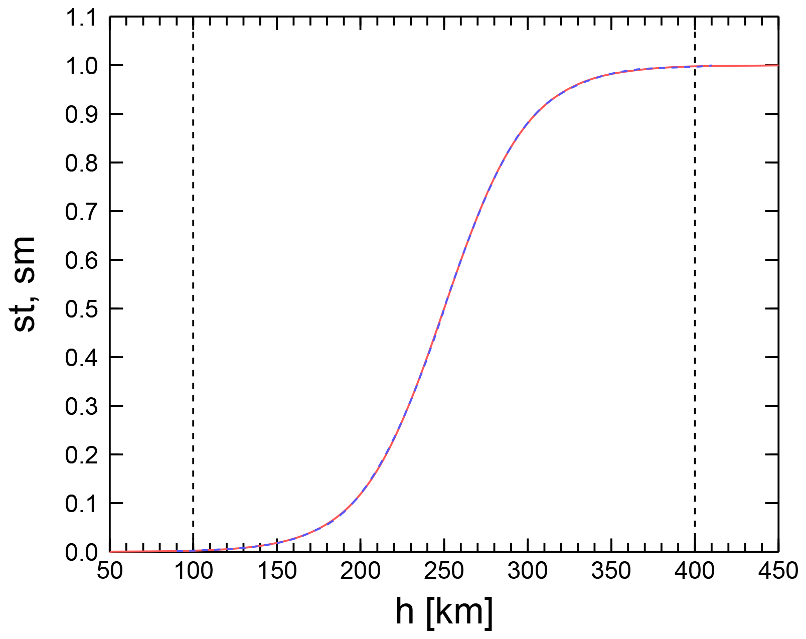
The φ component of the magnetic field in the entire interval for $\mathit{\theta }=\mathit{\pi }/\mathrm{6}$ is shown in Fig. 1. We use g₀=0.006, which corresponds to significant geomagnetic activity levels (Romashets and Vandas, 2020, 2022). The electric-current-density θ component from Eq. (16) is depicted in Fig. 2. The fit of the step-up function in the ionosphere is shown in Fig. 3.

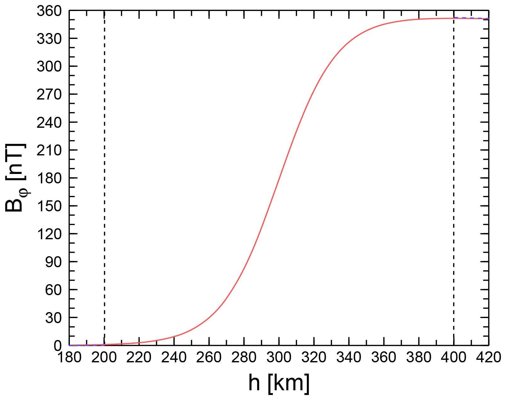
Figure 1 The φ component of the magnetic field in the ionosphere for $\mathit{\theta }=\mathit{\pi }/\mathrm{6}$ from Eq. (4). The interval (r_in,r_out) is marked by dashed vertical lines.

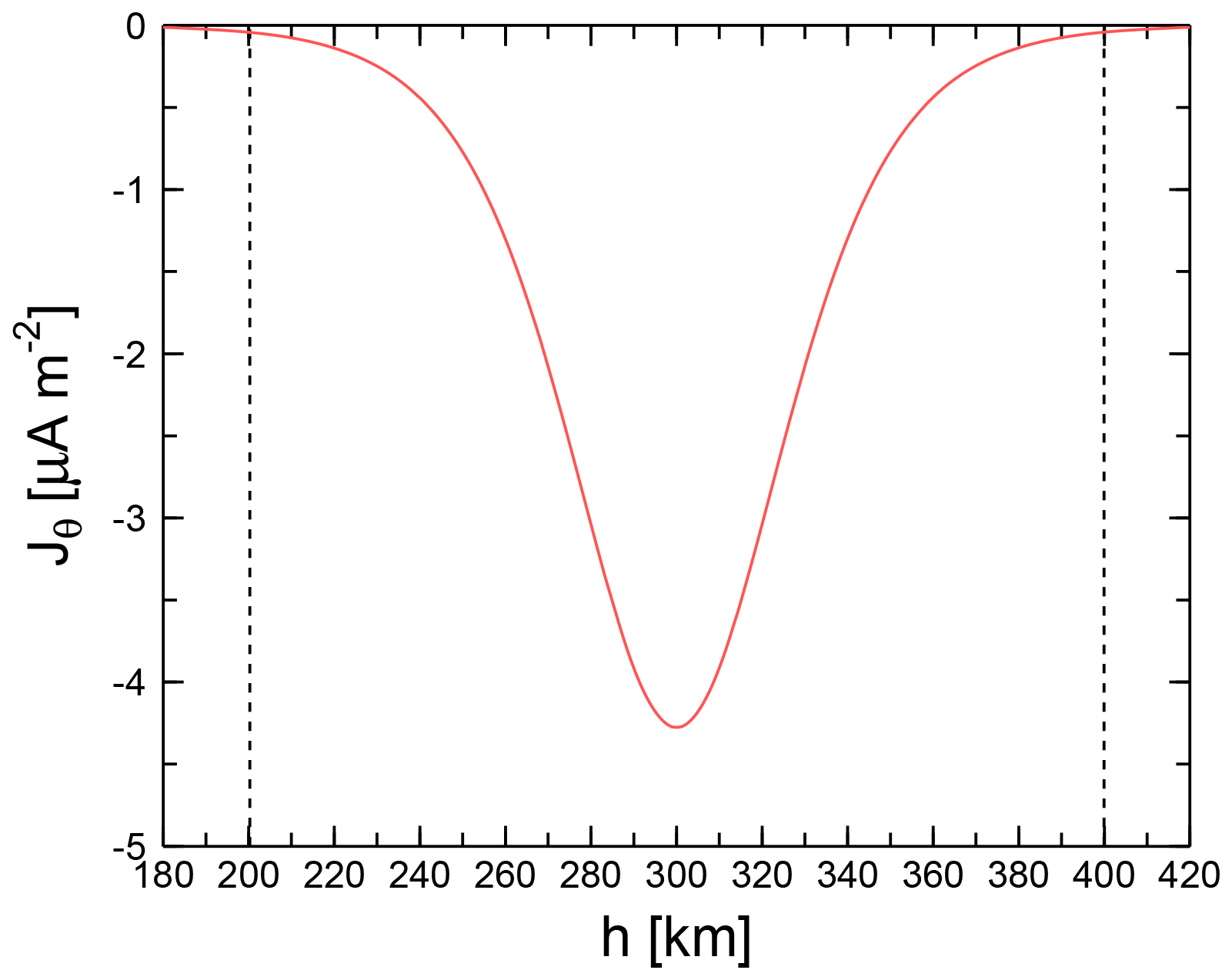
Figure 2 The θ component of the electric-current density in the ionosphere for $\mathit{\theta }=\mathit{\pi }/\mathrm{6}$ from Eq. (16). The interval (r_in,r_out) is marked by dashed vertical lines.

Figure 3 Fit of the step-up function of Eq. (7) (red line), obtained by a sum of power functions, as in Eq. (8) (dashed blue line), in the ionosphere. The interval (r_in,r_out) is marked by dashed vertical lines.

Using α from Eq. (1) and the rectified β value, we calculated the magnetic field using

$$\begin{array}{}\text{(17)}& \mathit{B}=\mathrm{\nabla }\mathit{\alpha }\times \mathrm{\nabla }\mathit{\beta }\end{array}$$

and numerical differentiation. The original φ component of the magnetic field – see Eq. (4) – is compared to that calculated with Eq. (17) in Fig. 4. The coincidence is excellent.

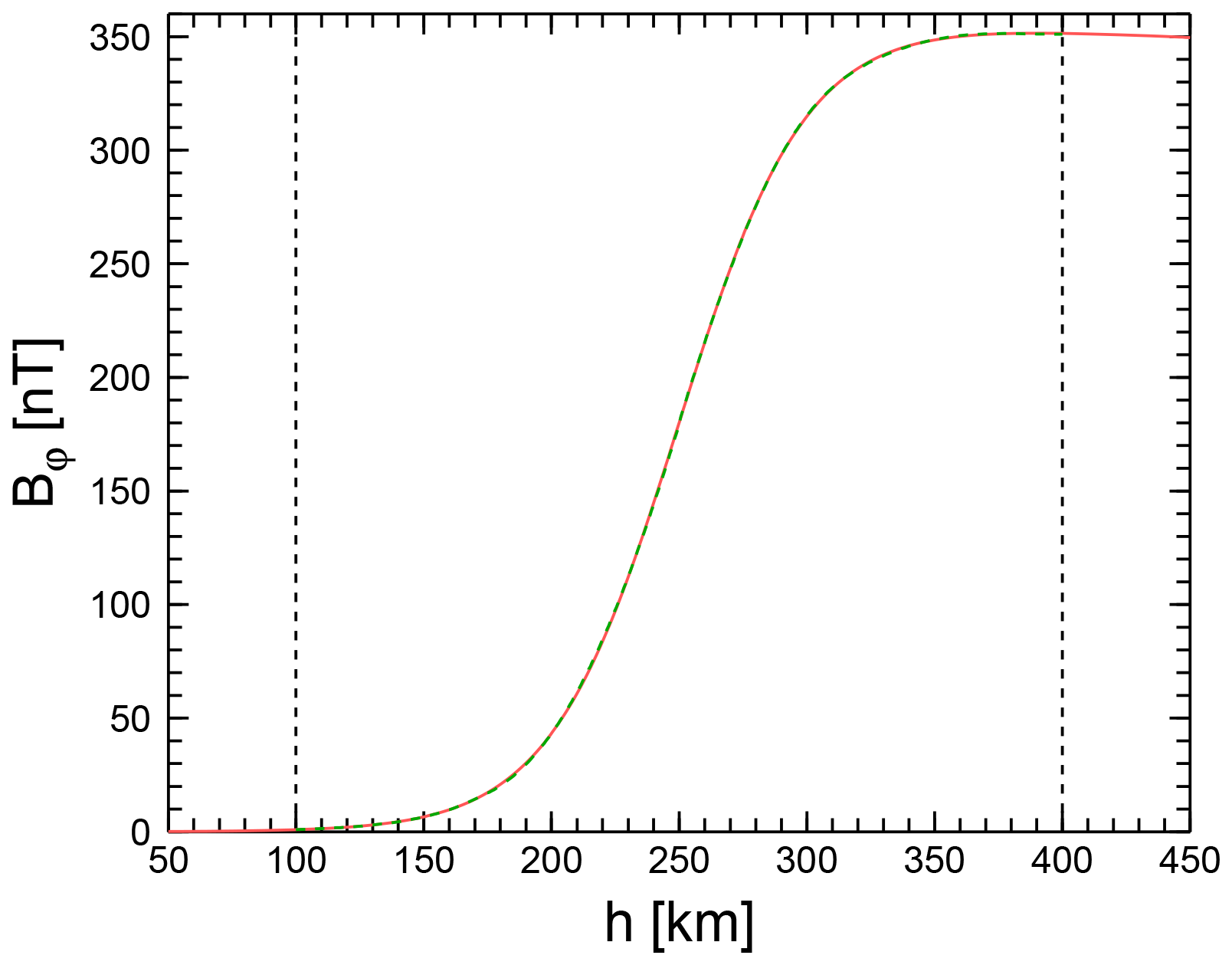
Figure 4 The given (red line) and modeled (dashed green line) φ component of the magnetic field in the ionosphere. The model B_φ was calculated from α and β by means of numerical differentiation. The interval (r_in,r_out) is marked by dashed vertical lines.

4 Discussion

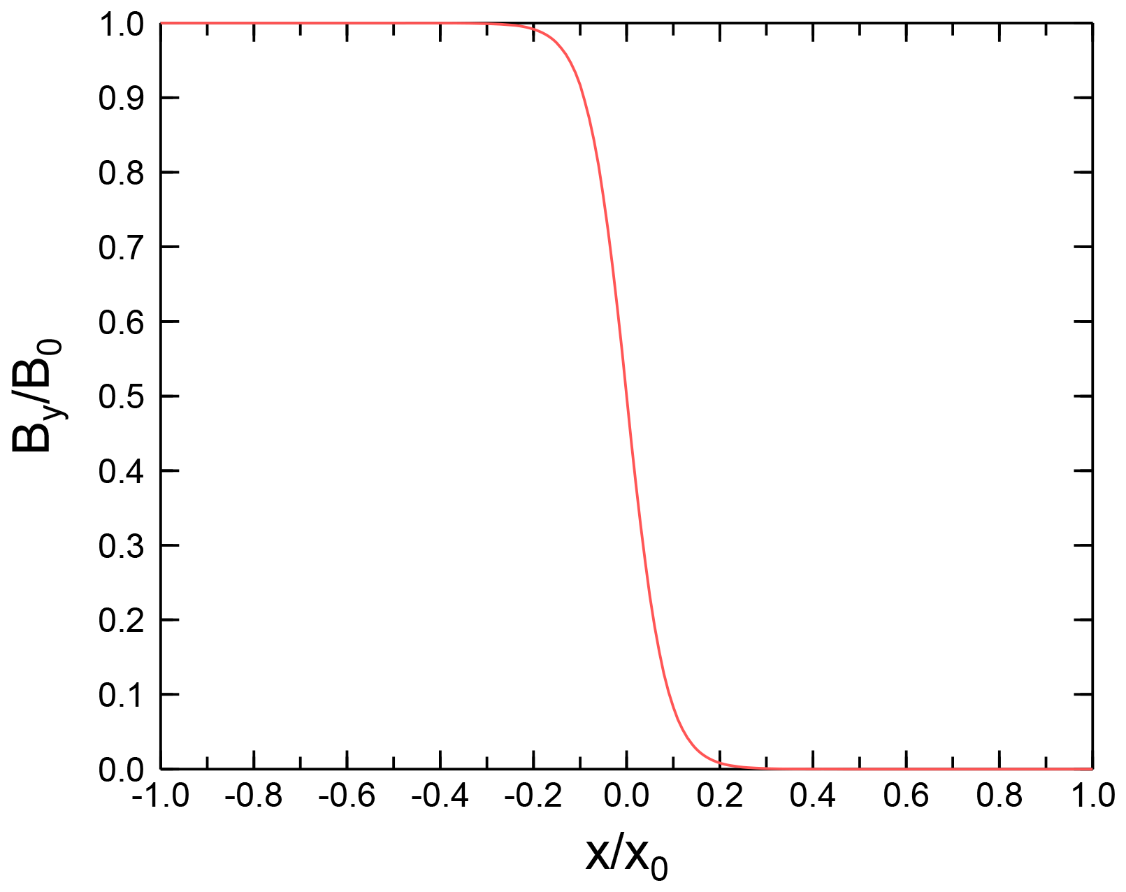
The transition from one region to another one in terms of Cartesian coordinates can demonstrate the approach better. Let us consider a planar layer $-x_{\mathrm{0}}<x<x_{\mathrm{0}}$. The pair of Euler potentials in the layer is as follows:

$$\begin{array}{}\text{(18)}& \mathit{\alpha }=B_{\mathrm{0}}\left(y-{\displaystyle \frac{x}{\mathrm{2}}}-{\displaystyle \frac{x_{\mathrm{0}}}{\mathrm{6}}}\log \cosh {\displaystyle \frac{\mathrm{3}x}{x_{\mathrm{0}}}}\right),\mathit{\beta }=z.\end{array}$$

Then, the y component of the magnetic field calculated with these α and β changes smoothly and has the following form:

$$\begin{array}{}\text{(19)}& B_y={\displaystyle \frac{\mathrm{1}}{\mathrm{2}}}{B}_{\mathrm{0}}\left(\mathrm{1}+\tanh {\displaystyle \frac{\mathrm{3}x}{x_{\mathrm{0}}}}\right).\end{array}$$

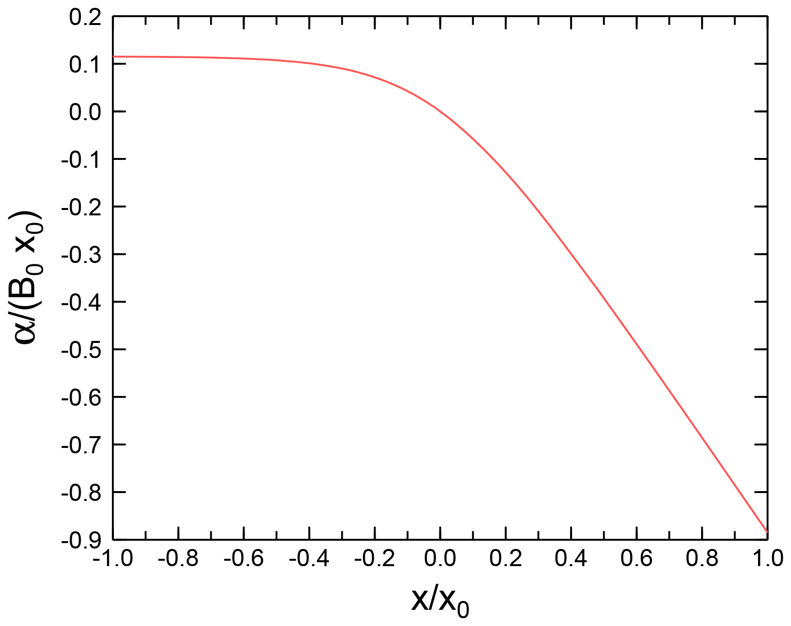
This magnetic-field component is plotted in Fig. 5. There is a smooth change from B_y≈0 at $x=-x_{\mathrm{0}}$ to B_y≈B₀ at x=x₀. The dependence of α on x is demonstrated in Fig. 6. The current density in the layer has only a z component,

$$\begin{array}{}\text{(20)}& J_z={\displaystyle \frac{\mathrm{3}{B}_{\mathrm{0}}}{\mathrm{2}{\mathit{\mu }}_{\mathrm{0}}}}{\displaystyle \frac{{\text{sech}}^{\mathrm{2}}\frac{\mathrm{3}x}{x_{\mathrm{0}}}}{x_{\mathrm{0}}}}.\end{array}$$

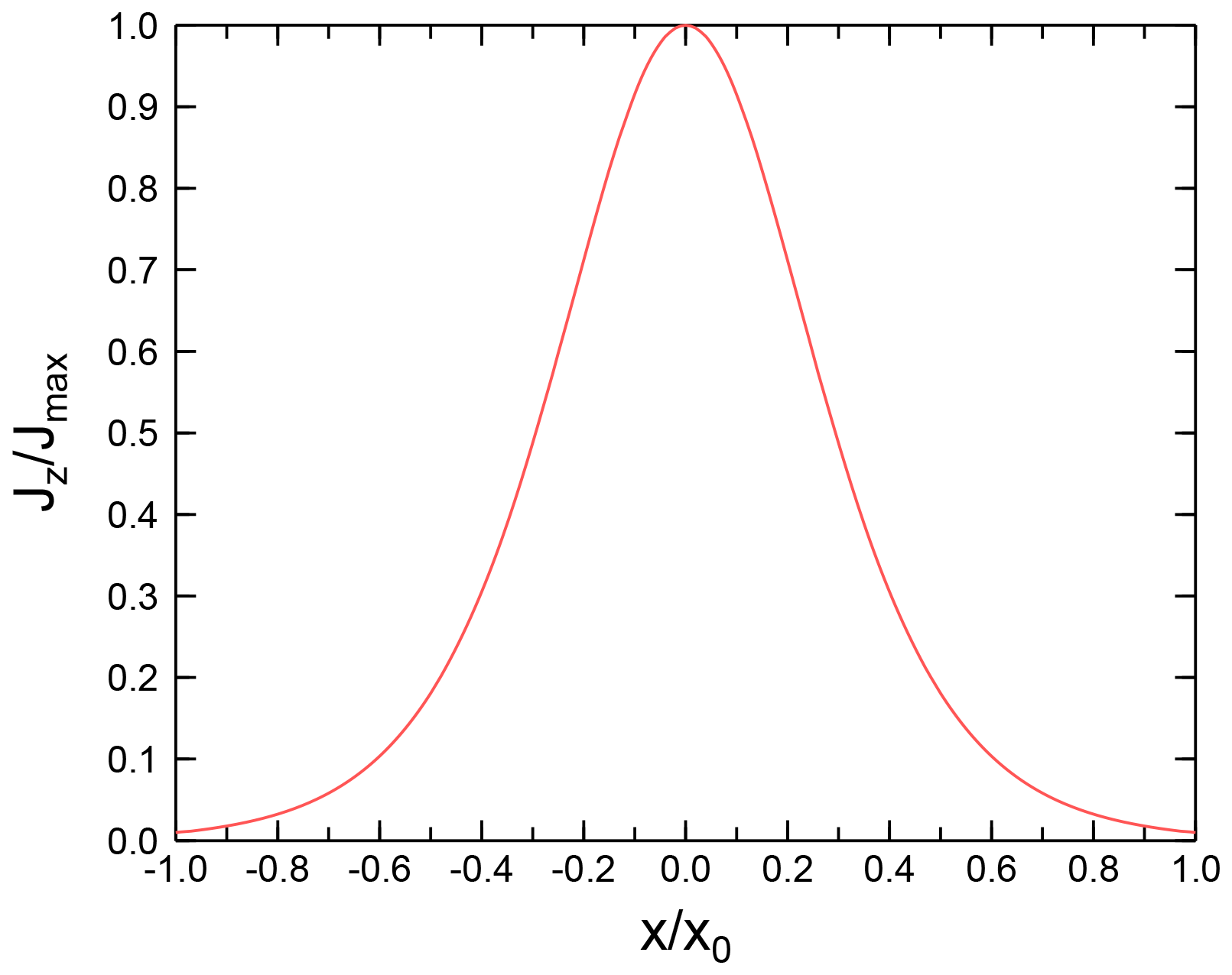
Its maximum (J_max) is reached in the middle of the layer. The profile of the electric-current-density z component given by Eq. (20) is depicted in Fig. 7. In Cartesian coordinates, one can easily deal with both of the tangential-to-the-layer coordinates and provide a smooth transition from their values in one region to those in another.

Figure 5 B_y in the layer.

Figure 6 Euler potential α in the layer for y=0.

Figure 7 Current density in the layer.

Returning to our spherical system in the ionosphere, it is interesting to see that, in addition to the toroidal component above the ionosphere, which is associated with the θ component of the current density in the ionosphere, we can also consider the transition of the poloidal (θ) component of the magnetic field. The magnetic field above the ionosphere is provided by the scalar potential Ψ, applicable for ${\mathit{\theta }}_{\mathrm{1}}>\mathit{\theta }>{\mathit{\theta }}_{\mathrm{2}}$, where the magnetic-field components are finite:

$$\begin{array}{}\text{(21)}& \mathrm{\Psi }=B_{\mathrm{0}}{r}_{\mathrm{0}}{g}_{\mathrm{0}}{\displaystyle \frac{\cos \mathit{\phi }\sqrt{\mathrm{1}-\cos \mathit{\theta }}}{\sqrt{\mathrm{1}+\cos \mathit{\theta }}}}.\end{array}$$

They are given by

$$\begin{array}{}\text{(22)}& {\displaystyle }{B}_r& {\displaystyle }=\mathrm{0},\text{(23)}& {\displaystyle }{B}_{\mathit{\theta }}& {\displaystyle }={\displaystyle \frac{B_{\mathrm{0}}{r}_{\mathrm{0}}{g}_{\mathrm{0}}\cos \mathit{\phi }}{r(\mathrm{1}+\cos \mathit{\theta })}},\text{(24)}& {\displaystyle }{B}_{\mathit{\phi }}& {\displaystyle }=-{\displaystyle \frac{B_{\mathrm{0}}{r}_{\mathrm{0}}{g}_{\mathrm{0}}\sin \mathit{\phi }\sqrt{\mathrm{1}-\cos \mathit{\theta }}}{r\sin \mathit{\theta }\sqrt{\mathrm{1}+\cos \mathit{\theta }}}}.\end{array}$$

This field is current-free. The magnetic field in the ionosphere has components as given by Eqs. (22)–(24), but with each multiplied by the function st from Eq. (7). In a similar fashion, as described in the Method section, the Euler potentials and current density in the ionosphere are found. Combining Eq. (3) and Eqs. (22)–(24), we can model locally a real ratio between Pedersen and Hall currents. The radial component is absent in Eqs. (22)–(24); this is a tangential discontinuity due to the special selection of the harmonic in Eq. (21), which does not depend on r.

The results of calculations depend on B_φ outside of the ionosphere; it is the input of the model. Different B_φ values will lead to different profiles in the ionosphere. We divide the ionosphere into four intervals, which enables us to consider inhomogeneities in the r direction. The tanh function is used for every interval. On the other hand, because the problem of finding the magnetic field in the ionosphere is solved locally, for specific φ and θ, this will describe inhomogeneities in the φ and θ directions as well.

5 Conclusions

It is important to construct the Euler potentials α and β for the study of charged-particle motion in a given medium. It is especially convenient to have α and β expressed in a compact analytical form. In this work, we found continuous Euler potentials in the finite-thickness contact discontinuity and applied them for the shell currents in the ionosphere. The result opens the way for studies of the fine structure of such kinds of discontinuities in solar wind, the magnetosphere, and interstellar space. The procedure consists of three steps. First, the magnetic field in the interface region is obtained, which represents a smooth transition from the magnetic field on one side to that on another side. Second, the region is divided into four parts, and the Euler potentials are derived for each of them. One of the potentials, α, is the same, but there are four β functions, one for each part of the interval. Next, because the addition of a function of α to β does not change the resulting magnetic field, we add needed functions to β functions in each part of the interval and provide continuity of β in the interface region (the ionosphere in our case) and at its boundaries.

Appendix A: Determination of coefficients c_i and rectification of β

We divide the interval 〈r_in,r_out〉 into four subintervals of equal length: 〈r_in,r₁₂〉, 〈r₁₂,r₂₃〉, 〈r₂₃,r₃₄〉, and 〈r₃₄,r_out〉, where $r_{\mathrm{12}}=r_{\text{in}}+(r_{\text{out}}-r_{\text{in}})/\mathrm{4}$, $r_{\mathrm{23}}=r_{\text{in}}+\mathrm{2}(r_{\text{out}}-r_{\text{in}})/\mathrm{4}$, and $r_{\mathrm{34}}=r_{\text{in}}+\mathrm{3}(r_{\text{out}}-r_{\text{in}})/\mathrm{4}$. For each subinterval, we determine the coefficients separately. Let us consider the first subinterval. We require

$$\begin{array}{}\text{(A1)}& {\displaystyle }\begin{array}{rl}{\displaystyle }& {\displaystyle }{\int }_{\frac{\mathrm{1}}{\mathrm{2}}(r_{\text{in}}+r_{\mathrm{12}})-\frac{\mathrm{1}}{\mathrm{6}}\mathrm{\Delta }r}^{\frac{\mathrm{1}}{\mathrm{2}}(r_{\text{in}}+r_{\mathrm{12}})+\frac{\mathrm{1}}{\mathrm{6}}\mathrm{\Delta }r}{\left[\text{sm}\left(r\right)-\text{st}\left(r\right)\right]}^{\mathrm{2}}\mathrm{d}r\\ {\displaystyle }& {\displaystyle }={\int }_{\frac{\mathrm{1}}{\mathrm{2}}(r_{\text{in}}+r_{\mathrm{12}})-\frac{\mathrm{1}}{\mathrm{6}}\mathrm{\Delta }r}^{\frac{\mathrm{1}}{\mathrm{2}}(r_{\text{in}}+r_{\mathrm{12}})+\frac{\mathrm{1}}{\mathrm{6}}\mathrm{\Delta }r}{\left[\sum _{i=\mathrm{1}}^I{c}_{\mathrm{1},i}{\left({\displaystyle \frac{r}{r_{\mathrm{0}}}}\right)}^{n_i}-\text{st}\left(r\right)\right]}^{\mathrm{2}}\mathrm{d}r\\ {\displaystyle }& {\displaystyle }=\text{min},\end{array}\end{array}$$

Figure A1 The Euler potential β (a) before and (b) after additions of the functions f(α).

where the integration is over an interval of length $\mathrm{\Delta }r/\mathrm{3}$, which symmetrically overlaps with the subinterval in play. Following the standard procedure for minimization, we differentiate Eq. (A1) by c_1,k and set it to zero, finally obtaining

$$\begin{array}{}\text{(A2)}& {\displaystyle }\begin{array}{rl}{\displaystyle }& {\displaystyle }{\sum }_{i=\mathrm{1}}^I{c}_{\mathrm{1},i}{\int }_{\frac{\mathrm{1}}{\mathrm{2}}(r_{\text{in}}+r_{\mathrm{12}})-\frac{\mathrm{1}}{\mathrm{6}}\mathrm{\Delta }r}^{\frac{\mathrm{1}}{\mathrm{2}}(r_{\text{in}}+r_{\mathrm{12}})+\frac{\mathrm{1}}{\mathrm{6}}\mathrm{\Delta }r}{\left({\displaystyle \frac{r}{r_{\mathrm{0}}}}\right)}^{n_i+n_k}\mathrm{d}r\\ {\displaystyle }& {\displaystyle }={\int }_{\frac{\mathrm{1}}{\mathrm{2}}(r_{\text{in}}+r_{\mathrm{12}})-\frac{\mathrm{1}}{\mathrm{6}}\mathrm{\Delta }r}^{\frac{\mathrm{1}}{\mathrm{2}}(r_{\text{in}}+r_{\mathrm{12}})+\frac{\mathrm{1}}{\mathrm{6}}\mathrm{\Delta }r}\text{st}\left(r\right){\left({\displaystyle \frac{r}{r_{\mathrm{0}}}}\right)}^{n_k}\mathrm{d}r,\end{array}\end{array}$$

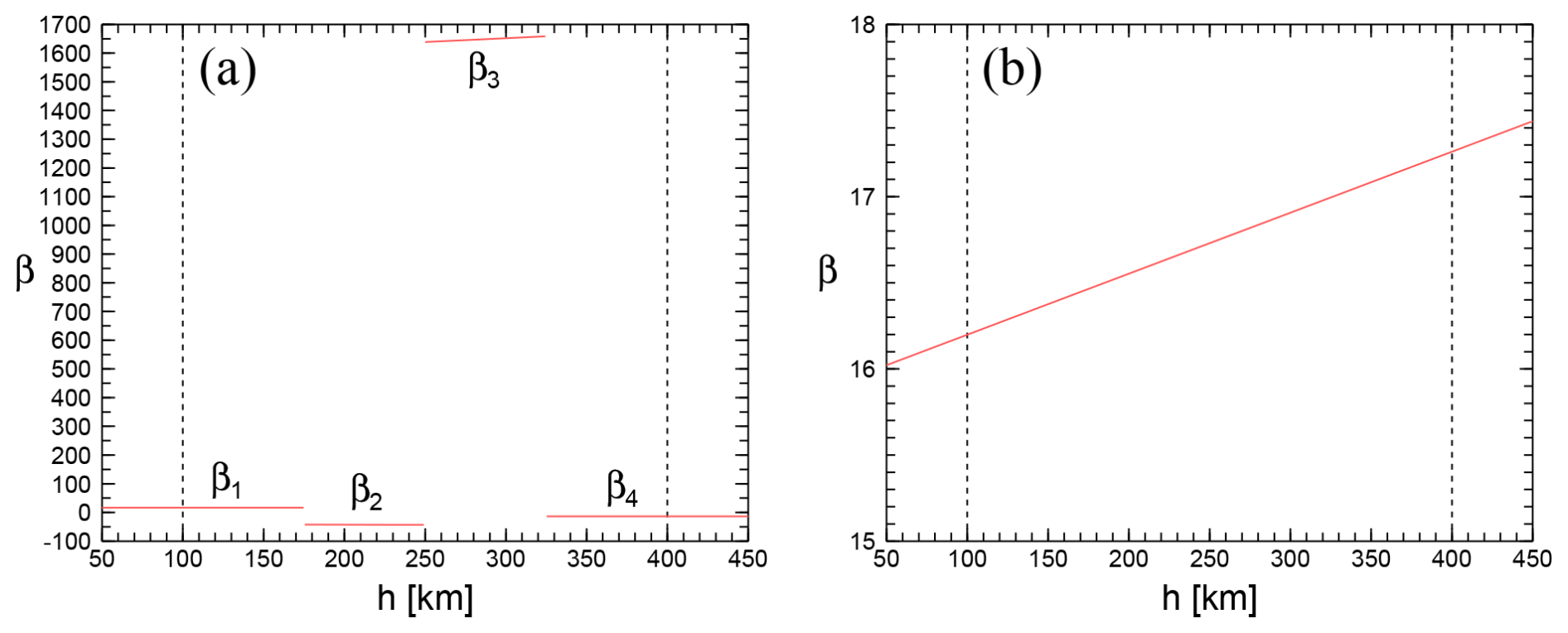
which, for $k=\mathrm{1},\mathrm{\dots },I$, represents a set of linear equations that are solved for c_1,i. The integrals on the left-hand side of Eq. (A2) can be calculated analytically. We proceed in the same way for the remaining subintervals 2–4 and thus obtain four sets of the c_i coefficients, which determine four functions, β₁, β₂, β₃, and β₄, by means of Eq. (13). These functions are independent, and one cannot expect that neighboring β functions will have the same values at the interface (e.g., β₁ and β₂ at r₁₂); Fig. A1a demonstrates this.

To make β continuous in the whole interval 〈r_in,r_out〉, we follow a procedure of rectification described in Vandas and Romashets (2024). This procedure relies on the fact that, when a function of α is added to β, it has no effect on the related magnetic field. We define β=β₁ for r<r₁₂. The β₂ value is adjusted in the following way. The α value at the interface r₁₂, $\mathit{\alpha }=B_{\mathrm{0}}{r}_{\mathrm{0}}^{\mathrm{3}}{\sin }^{\mathrm{2}}\mathit{\theta }/r_{\mathrm{12}}$, is a function of θ only. We introduce its inverse function:

$$\begin{array}{}\text{(A3)}& {\mathit{\theta }}_{\mathrm{12}}\left(\mathit{\alpha }\right)=\arcsin \sqrt{{\displaystyle \frac{\mathit{\alpha }{r}_{\mathrm{12}}}{B_{\mathrm{0}}{r}_{\mathrm{0}}^{\mathrm{3}}}}}.\end{array}$$

The adjusted β₂ value, denoted as β_2a, is

$$\begin{array}{}\text{(A4)}& {\displaystyle }\begin{array}{rl}{\displaystyle }{\mathit{\beta }}_{\text{2a}}(r,\mathit{\theta },\mathit{\phi })=& {\displaystyle }{\mathit{\beta }}_{\mathrm{2}}(r,\mathit{\theta },\mathit{\phi })+{\mathit{\beta }}_{\mathrm{1}}\mathit{\{}{r}_{\mathrm{12}},{\mathit{\theta }}_{\mathrm{12}}[\mathit{\alpha }(r,\mathit{\theta })],\mathrm{0}\mathit{\}}\\ {\displaystyle }& {\displaystyle }-{\mathit{\beta }}_{\mathrm{2}}\mathit{\{}{r}_{\mathrm{12}},{\mathit{\theta }}_{\mathrm{12}}[\mathit{\alpha }(r,\mathit{\theta })],\mathrm{0}\mathit{\}}.\end{array}\end{array}$$

We define β=β_2a for $r\in 〈r_{\mathrm{12}},r_{\mathrm{23}}〉$. Similarly, the adjusted β₃ value is

$$\begin{array}{}\text{(A5)}& {\displaystyle }\begin{array}{rl}{\displaystyle }{\mathit{\beta }}_{\text{3a}}(r,\mathit{\theta },\mathit{\phi })=& {\displaystyle }{\mathit{\beta }}_{\mathrm{3}}(r,\mathit{\theta },\mathit{\phi })+{\mathit{\beta }}_{\text{2a}}\mathit{\{}{r}_{\mathrm{23}},{\mathit{\theta }}_{\mathrm{23}}[\mathit{\alpha }(r,\mathit{\theta })],\mathrm{0}\mathit{\}}\\ {\displaystyle }& {\displaystyle }-{\mathit{\beta }}_{\mathrm{3}}\mathit{\{}{r}_{\mathrm{23}},{\mathit{\theta }}_{\mathrm{23}}[\mathit{\alpha }(r,\mathit{\theta })],\mathrm{0}\mathit{\}},\end{array}\end{array}$$

and this is analogically the case for β_4a. We define β=β_3a for $r\in 〈r_{\mathrm{23}},r_{\mathrm{34}}〉$ and β=β_4a for r>r₃₄. This rectified β is shown in Fig. A1b.