Characteristic analysis of the differences between total electron content (TEC) values in global ionosphere map (GIM) grids

Using total electron content (TEC) from a global ionosphere map (GIM) for ionospheric delay correction is a common method of eliminating ionospheric errors in satellite navigation and positioning. On this basis, the TEC of a puncture point can be obtained by GIM grid TEC interpolation. However, in terms of grid, only few studies have analyzed the TEC value size characteristics of its four grid points, that is, the TEC difference characteristics among them. In view of this, by utilizing the GIM data from high solar-activity years (2014) and low solar-activity years (2021) provided by CODE (Center for Orbit Determination in Europe), this paper proposes the grid TEC difference as a way of analyzing TEC variation characteristics within the grid, which is conducive to exploring and analyzing the variation characteristics of the ionosphere TEC in the single-station area. The value is larger in high solar-activity years and generally small in low solar-activity years, and the value of high-latitude areas is always smaller than that of low-latitude areas. Specifically, in high solar-activity years, most of the GIM grid TEC internal differences are within 4 TECu (1 TECu = 10¹⁶ electrons m⁻²) in high-latitude and midlatitude regions, while only 78.17 % are in low-latitude regions. In low solar-activity years, the TEC difference values within a GIM grid are mostly less than 2 TECu, and most of them in the high and middle latitudes are within 1 TECu. The main finding of this analysis is that the grid TEC differences are small for most GIM grids, especially in the midlatitudes to high latitudes of low solar years. This means that relevant extraction methods and processes can be simplified when TEC within these GIM grids is needed.

1 Introduction

Ionospheric delay is an important error source in navigation, positioning and timing of a global navigation satellite system (GNSS) (Hernández-Pajares et al., 2018; Hu et al., 2018; Jin et al., 2015), which affects the accuracy of the GNSS on the one hand. On the other hand, global all-weather observations of GNSS can be fully used to construct a global ionospheric model (Chen et al., 2020; Hernández-Pajares et al., 2009, 2011). Combined with total electron content (TEC) parameterized by ionospheric delay, the global ionosphere map (GIM) can be generated by TEC modeling based on the globally distributed GNSS observations (Mannucci et al., 1998; Schaer, 1999; Hernández-Pajares et al., 2017; Zhang and Zhao, 2018). The GIM can be mainly applied in the following fields: (1) the TEC provided by GIM for ionospheric delay correction is a common method to eliminate ionospheric errors in satellite navigation and positioning (Rovira-Garcia et al., 2019; Su et al., 2019); (2) the GIM can be employed to eliminate TEC parameters in GNSS observation equations, thereby obtaining the code bias parameters of satellites and receivers (Montenbruck et al., 2014; Li et al., 2017); (3) the GIM can be adopted to analyze and study the characteristics of global or regional ionospheric variations (Feng et al., 2022, 2023). It should be mentioned that the above applications need to focus on the grid TEC information. For example, when performing ionospheric delay correction, the TEC value of the puncture point needs to be obtained by interpolating the TEC of the grid where the puncture point is located (Jin et al., 2012). Therefore, taking the GIM grid as an object, it is meaningful to analyze the variation in TEC difference within the grid, which further facilitates a more in-depth understanding of the variation characteristics of the ionosphere in the single-station region.

Since the ionosphere is influenced by solar activity, its system state and variation are complicated. A number of studies worldwide have demonstrated that the ionosphere exhibits equatorial anomalies and latitudinal effects in space and, at the same time, periodic variations with high and low solar activity in time (Tariq et al., 2020; Muafiry et al., 2022; Yu et al., 2014; Kalinin and Khotenko, 2012). In addition, the GIM has also been utilized to conduct relevant research on the spatiotemporal variation characteristics of the regional ionospheric TEC (Guo et al., 2017). However, most of the studies on the ionospheric TEC variation characteristics focus on large scales. Considering that the ionospheric penetration point region formed by GNSS observation at a single station may contain several adjacent grids, the characteristics of the ionospheric TEC variation in such a single station area are rarely analyzed, especially in grid units. Moreover, using TEC from a GIM for ionospheric delay correction is a common method of eliminating ionospheric errors in satellite navigation and positioning. With the aid of the method, the TEC of a puncture point can be obtained by GIM grid TEC interpolation. However, in terms of grids, few studies have been performed to analyze the TEC difference characteristics of its four grid points. Hence, an accurate and comprehensive analysis of the variation in TEC difference in grids is of great importance, which is helpful to understand the variation characteristics of the ionosphere in the single-station area.

Given this, the grid TEC difference is proposed as a means of analyzing TEC variation characteristics within the grid. The GIM data for 2 years from high solar activity (2014) and low solar activity (2021) provided by CODE (Center for Orbit Determination in Europe) are selected to calculate the TEC difference for each grid point in this paper. Based on the calculation of the spatial and temporal variations in the difference values, both spatial and temporal characteristics of the TEC difference values of the four grid points within the grid are analyzed in detail.

This paper is organized as follows. In Sect. 2, related methods and data are introduced, especially the definition and calculation of grid TEC differences. In Sect. 3, the spatial and temporal characteristics of the TEC difference values of the four grid points within the grid are analyzed. Section 4 presents the conclusions of this paper.

2 Method and data

2.1 Grid TEC

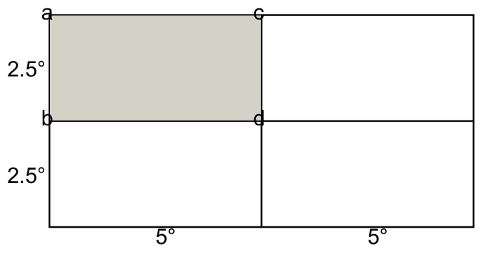
The GIM provided by CODE plays an important role in ionospheric research. By using globally distributed International GNSS Service (IGS) tracking stations, the GIM can be employed to generate a grid TEC model with 5^∘ longitude and 2.5^∘ latitude by spherical harmonic function modeling. Previously CODE's GIM was a grid map at 2 h intervals, with a day divided into 13 maps, while the interval of the current GIM is 1 h, with 25 maps per day.

Figure 1 shows a schematic diagram of GIM grids with a 5^∘ interval in the longitude direction and a 2.5^∘ interval in the latitude direction, each of which has four grid points (marked a, b, c and d in Fig. 1), indicating that there are 70×72 grids and 71×73 grid point TEC values in each TEC map. The grid TEC described in this paper refers to the TEC value of a grid, which includes the TEC value of the four grid points and the TEC value inside the grid. In practice, the grid TEC value is variable, but the GIM-provided grid TEC only has four grid point values. It should be noted that the analysis in this paper is based on the GIM and does not consider the problem of low TEC accuracy in some areas due to uneven or insufficient GNSS tracking stations.

Figure 1 The GIM grid diagram.

For a particular grid, the TEC of a certain point inside it is calculated by the four grid point TECs of the grid, which is also known as interpolation calculation. Figure 2 shows the distribution of puncture points in ABPO (GNSS tracking station). It can be seen that the puncture points are in a particular grid. A particular puncture point is in a particular grid, and its TEC value is obtained by interpolating the TEC of the four grid points when using GIM for ionospheric delay correction or TEC elimination. Therefore, understanding the variation in TEC values in these grids can not only provide a theoretical reference for obtaining the TEC values of the puncture point but also acquire the information on variation characteristics of the ionosphere in the area of a single GNSS station. In other words, this understanding also allows us to analyze the spatial and temporal variation characteristics of the four grid point TECs of each grid.

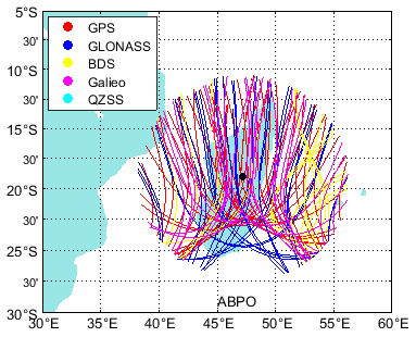
Figure 2 Distribution of puncture points in ABPO (different colors show the path of the puncture point formed by the observations of different satellites, and the black circle indicates the location of the station).

2.2 Grid TEC difference

In this paper, the grid TEC difference is proposed as a means of analyzing the TEC variation characteristics within the grid. The grid TEC difference includes the difference on the spatial scale and the difference on the temporal scale. The former is defined as the difference between the four grid points of a grid, and the latter is defined as the difference between four grid points on the grids of two adjacent GIMs. Specifically, on the premise of treating these grids as units, through calculating the grid TEC difference values of each grid, the variation in TEC difference values within these grids in space and time is counted, and both spatial and temporal variation characteristics of TEC difference values of four grid points within the grids are analyzed.

On the spatial scale, the grid difference values of each GIM are firstly calculated as shown in Eq. (1), and the maximum, average and minimum values of TEC difference values of each grid are counted. Afterwards, the spatial variation characteristics of grid difference values in different periods are analyzed. Finally, the variation pattern of TEC difference values of a grid on a particular day is obtained. The grid TEC difference on the spatial scale can be expressed as

$$\begin{array}{}\text{(1)}& \mathrm{\Delta }{T}_{jk}=\left|T_j-T_k\right|j=\left\{a,a,a,b,b,c\right\}k=\left\{b,c,d,c,d,d\right\},\end{array}$$

where T_j and T_k are the TEC of grid points j and k, respectively, and ΔT_jk is the grid TEC difference; there are six ΔT in each grid.

On the temporal scale, the grid difference values between adjacent moments of each GIM are calculated as shown in Eq. (2), and the maximum, average and minimum values of TEC difference values of each grid are also counted. Then, the temporal variation characteristics of grid difference values in different periods are analyzed. Finally, the variation pattern of TEC difference values of a grid on a particular day is achieved. The grid TEC difference on a timescale can be expressed as

$$\begin{array}{}\text{(2)}& \mathrm{\Delta }{T}_j^n=\left|T_j^{n+\mathrm{1}}-T_j^n\right|j=\left\{a,b,c,d\right\},\end{array}$$

where $T_j^n$ is the TEC of grid point j for the nth GIM map, n=12 in 2014 and n=24 in 2021, and $\mathrm{\Delta }{T}_j^n$ is the TEC difference between grid point between adjacent maps; there are four ΔT in each grid.

Since the TEC of the puncture point is interpolated through the grid point, it is crucial to analyze the variation in TEC difference in the grid, which contributes to gaining insight into the variation characteristics of the ionosphere in the single-station area. Moreover, understanding the characteristics of TEC difference in a grid can provide a simplified idea for obtaining TEC at puncture points.

2.3 Data

The GIM produced by CODE is used as the analysis data for this paper. Considering that ionospheric changes are influenced by solar activity, the F10.7 index is utilized to reflect the degree of solar activity. The monthly average F10.7 index changes from 2010 to 2021 are collected, as shown in Fig. 3. From the figure, it can be seen that the highest F10.7 index in 2014 represented a high solar-activity year.

Figure 3 Average monthly F10.7 index from 2010 to 2021.

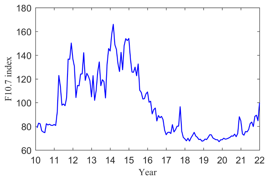
In order to distinguish the TEC changes in high and low solar-activity years, the GIM data for 2014 (high solar-activity year) and 2021 (low solar-activity year) are selected for analysis in this paper. There are 25 maps for 19 October 2014 and the day after, with 365 d in the year, and all GIM graphs with 2 h interval are selected for the unified analysis of 2014. However, the 300th day of the 2021 data file is corrupted, suggesting there are 364 d of data available for that year.

3 Results and analysis

3.1 Spatial variation

The data for 2014 and 2021 are used to make differences between the grid TECs of each GIM, with six differences for each grid. In order to analyze the variation in the grid TEC difference, the GIM of an arbitrary day (DOY112) is selected, and the maximum, mean and minimum values of the absolute values of the grid TEC difference are counted. The results of the variation with latitude at four moments of the day (2, 8, 14 and 20) are summarized in Fig. 4. The maximum, mean and minimum values are indicated by three colors, and their mean values are also marked on the graph by three colors. The first and second rows denote the results for 2014 and 2021, respectively, and the first to fourth columns represent the results for the four moments, respectively.

As can be seen from Fig. 4, the maximum, mean and minimum values of the absolute value of the grid TEC difference are larger and show a bimodal variation in the low-latitude region. This is because of the sudden increase in the TEC value of the grid point at 30^∘ in the GIM, resulting in a large grid TEC difference near 30^∘ N and 30^∘ S. Although the TEC values of grid points between 30^∘ N and 30^∘ S are large, their differences are small, leading to the bimodal phenomenon in the figure. The reason is that due to active variation in the ionosphere at low latitudes, its TEC shows large values, and the grid TEC difference increases abruptly near 30^∘ N and 30^∘ S. Comparing the results of the 2 years, the grid TEC difference is larger in 2014. In the meantime, it is evident from their mean values that the ionospheric variability is more active in high solar-activity years, with larger differences between the grid TECs exhibited. Through observation, all figures present the gradual increase in the variation in the grid TEC difference from high to low latitudes, indicating that the variation in the grid TEC difference is closely associated with the latitude at which the grid TEC is located.

Like Fig. 4, the variation in the GIM grid TEC difference in longitude is shown in Fig. 5. It is obvious that the change in grid TEC difference has no obvious characteristics in the direction of longitude, which is different from Fig. 4. This indicates that the change in grid TEC difference has a certain relationship with latitude. Therefore, subsequent analyses are mainly in the latitudinal direction.

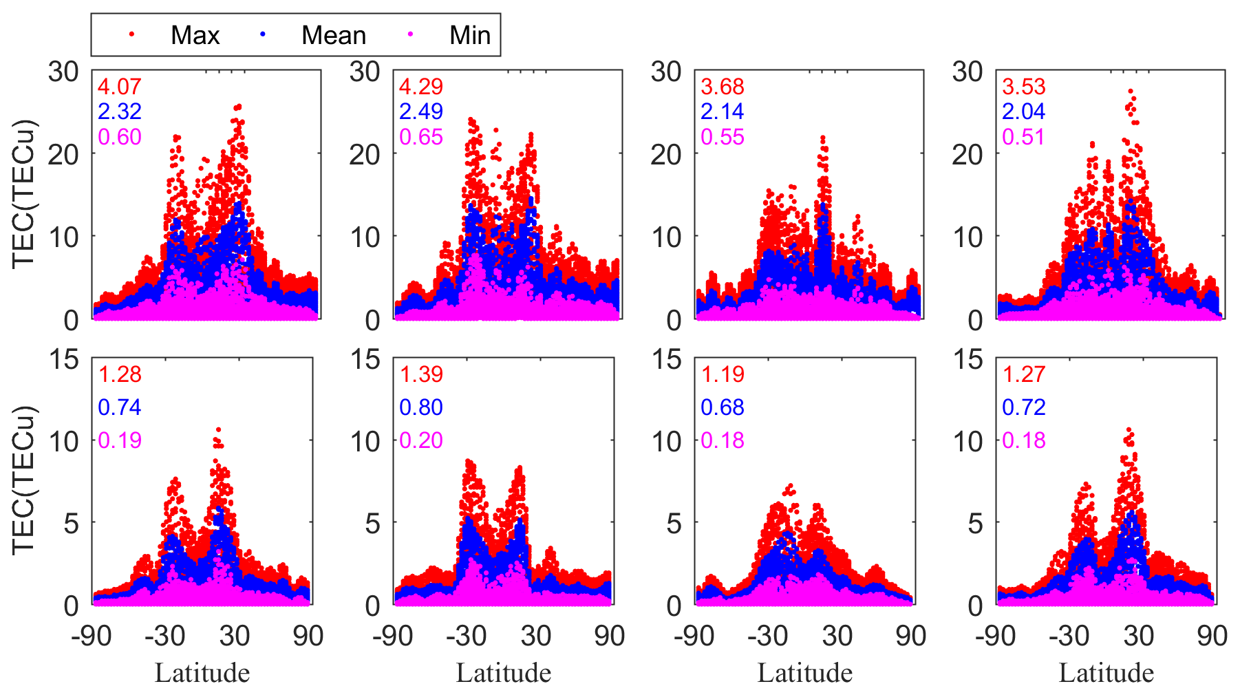
Figure 4 Variation in GIM grid TEC difference in latitude (the first and second rows denote the results for 2014 and 2021, respectively, and the first to fourth columns represent the results for the four moments, respectively).

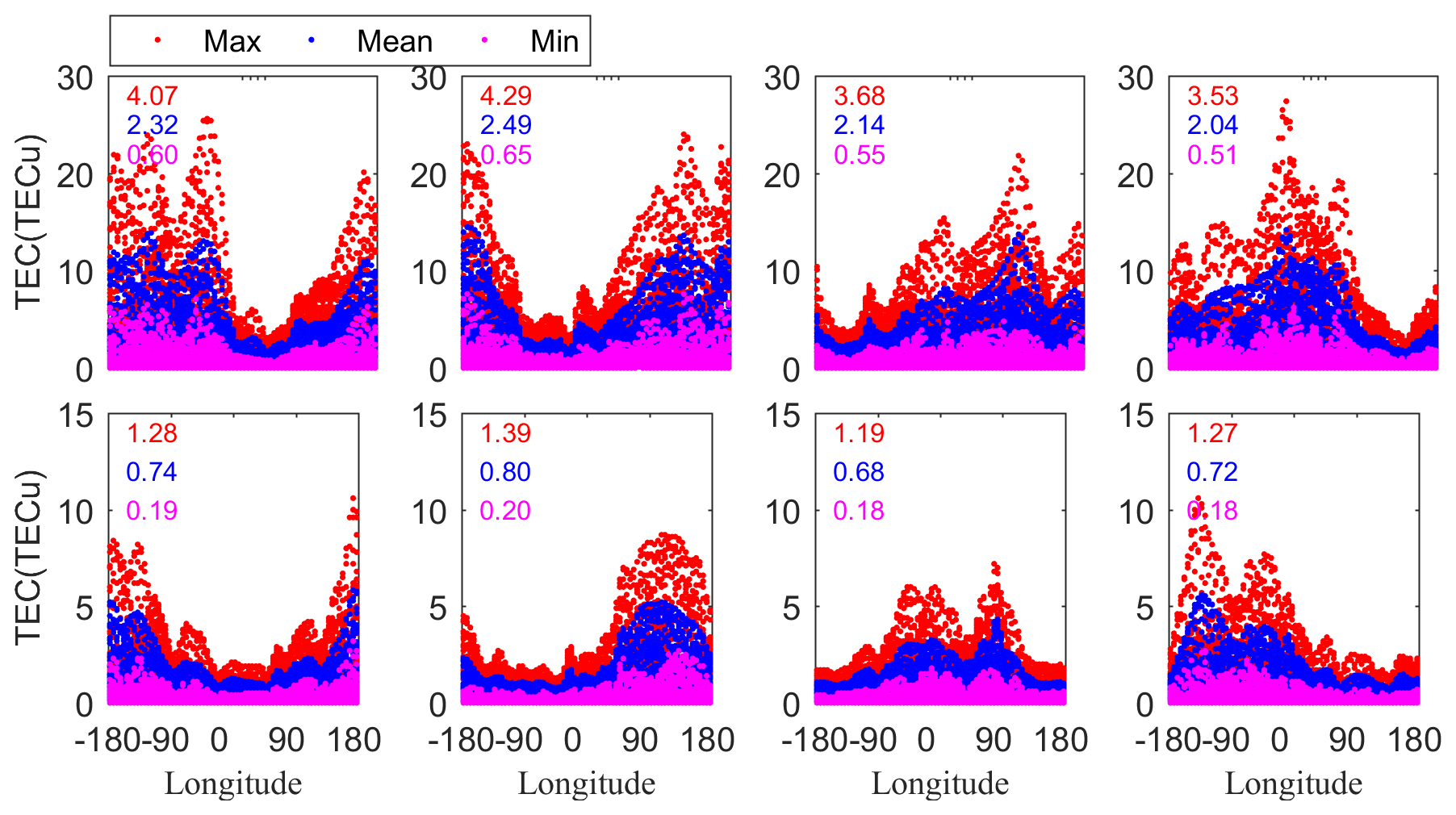
Figure 5 Variation in GIM grid TEC difference in longitude (the first and second rows denote the results for 2014 and 2021, respectively, and the first to fourth columns represent the results for the four moments of the day – 2, 8, 14 and 20 – respectively).

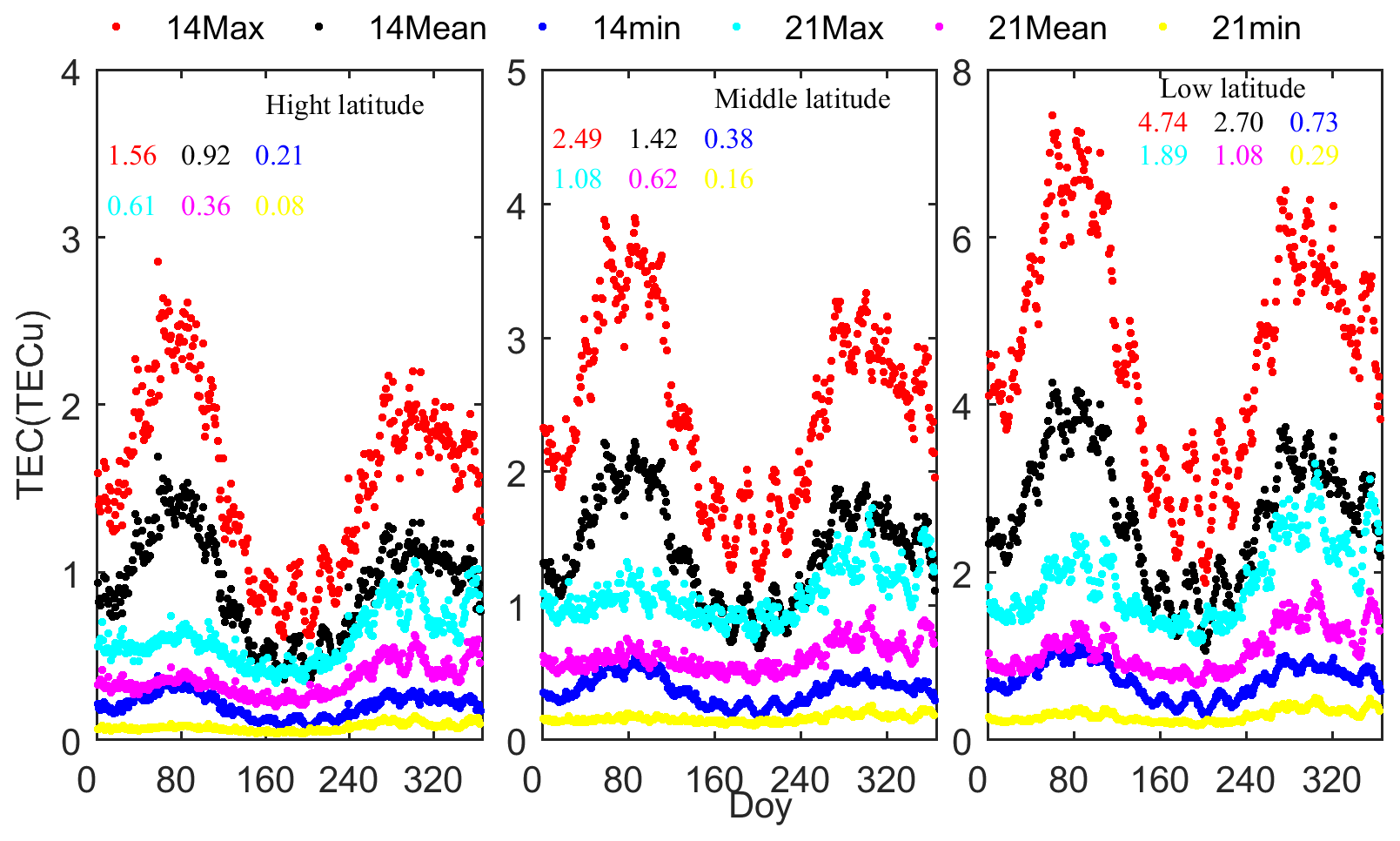
To further analyze the variation in grid TEC differences over the year, the GIM grids are counted separately according to high latitudes, midlatitudes and low latitudes, with 22, 24 and 24 grids per map, respectively. The maximum, mean and minimum values of grid TEC differences are averaged over 13 or 25 GIMs of a day at high, middle and low latitudes. It should be noted that the difference values of the statistics here are regarded as absolute values. The results of the statistics are tabulated in Fig. 6, where the maximum, mean and minimum values of TEC differences between the grid in 2014 and 2021 are indicated by six colors, and their mean values for 1 year are also represented on the graph by different colors. From the figure, the maximum, mean and minimum values of grid TEC differences in 2014 show obvious fluctuations in all three regions. Especially the maximum and mean values increase and decrease twice, which may be related to ionospheric activity. This trend is the same as the trend of F10.7 in 2014 in Fig. 3. Nevertheless, F10.7 in 2021 displays a slower trend of variation. In the low solar-activity year, the maximum, mean and minimum values of the grid TEC difference in Fig. 4 also show a slower annual variation trend. Among the three latitudes, the low latitudes are more active, while both high latitudes and midlatitudes are relatively flat. The daily average value of the maximum grid TEC difference is close to 8 TECu (1 TECu = 10¹⁶ electrons m⁻²)in 2014 and around 4 TECu in 2021, while that value is within 4 and 3 TECu at midlatitudes and high latitudes, respectively. For the minimum value of the gridded TEC difference, the mean values are within 2 TECu for both years. This indicates that the factors affecting the magnitude of the GIM grid TEC difference mainly include solar activity and the latitude at which the grid is located.

Figure 6 Annual variation in grid TEC difference in GIMs.

Figure 7 Histogram of grid TEC difference in temporal variation.

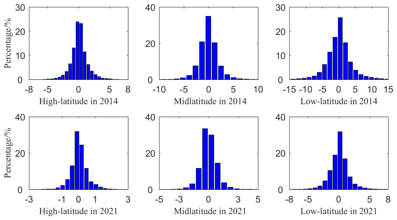
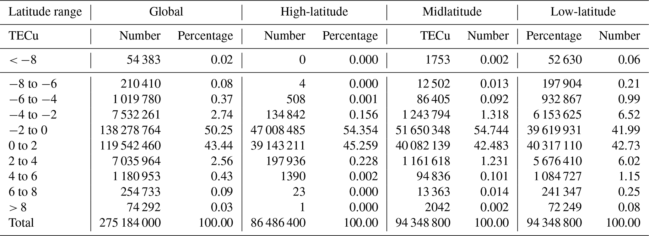
For further analysis, the TEC difference in all grids in a year is counted, and there are six differences for each grid. In 2014, all the grids are counted at 2 h intervals on 13 maps a day, and there are $\mathrm{6}\times \mathrm{70}\times \mathrm{72}\times \mathrm{13}\times \mathrm{365}=\mathrm{14}\mathrm{3488}\mathrm{800}$ differences; in 2021, the grids are counted at 1 h intervals on 25 maps a day, and there are $\mathrm{6}\times \mathrm{70}\times \mathrm{72}\times \mathrm{25}\times \mathrm{364}=\mathrm{27}\mathrm{5184}\mathrm{000}$ differences. As in the previous section, the frequency of grid TEC differences between −8 and 8 TECu at 2 TECu intervals is still counted separately according to high and low latitudes. The statistical results for 2014 and 2021 are organized in Tables 1 and 2. The histograms of TEC grid differences according to each of the three latitudes are depicted in Fig. 7.

Figure 8 Annual variation in grid TEC difference in GIMs.

Figure 9 Histogram of grid TEC difference in spatial variation.

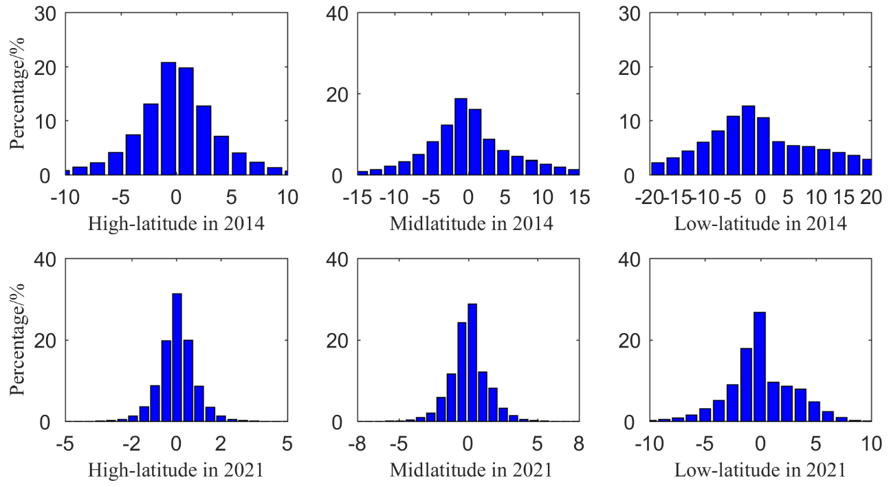
As can be seen from the results in Table 1, 72.11 % of the 2014 GIM grid TEC differences are in the range of −2 to 2 TECu, 87.75 % of the grid TEC differences are in the range of −2 to 2 TECu in the high-latitude region, and the values of grid TEC differences account for 76.71 % and 53.19 % in midlatitude and low-latitude regions, respectively. Moreover, 90.20 % of the grid TEC differences are in the range of −4 to 4 TECu for 2014 GIM, while the values of grid TEC differences account for 98.38 %, 94.73 % and 78.17 % in high-latitude, midlatitude and low-latitude regions, respectively. Obviously, the TEC difference values present a relatively larger variation trend in the low-latitude region in 2014. This is attributed to more active ionospheric variability in the high solar-activity year of 2014 in the low-latitude region, which is also consistent with the results of the previous analysis.

Table 1 Statistics of GIM grid TEC difference in 2014.

From the results in Table 2, 93.69 % of the GIM grid TEC difference values in 2021 are in the range of −2 to 2 TECu. Overall, 99.61 % of the grid TEC difference values in the range of −2 to 2 TECu are in the high-latitude region, while 97.22 % and 84.72 % of TEC difference values in the range of −2 to 2 TECu are in midlatitude and low-latitude regions, respectively. Moreover, 98.99 % of the GIM in 2021 for grid TEC differences are in the range of −4 to 4 TECu, and 99.99 %, 99.78 % and 97.26 % for high-latitude, midlatitude and low-latitude regions, respectively. Clearly, the range of GIM grid TEC difference is larger in the range of −2 to 2 TECu in 2021 compared to 2014. Most of the grid TEC differences are less than 2 TECu in low solar-activity years like 2021, and almost all grid TEC differences are within 4 TECu, which is related to the flattening of the ionospheric activity due to lower solar activity.

Table 2 Statistics of GIM grid TEC difference in 2021.

The histogram of grid TEC differences in Fig. 7 also reveals that a larger proportion of high-latitude and midlatitude regions have a smaller range of TEC differences than low-latitude regions, and a larger proportion of 2021 has a smaller range of TEC differences than 2014. In addition, the GIM grid TEC differences all follow a normal distribution, and most of the grid TEC differences are within a certain range, especially for the high-latitude region in 2021. It can be found that most of its grid TEC differences are within 1 TECu, and most of its midlatitude region is also within 2 TECu. In summary, the TEC differences in the GIM grid are smaller in the high-latitude and midlatitude regions where the ionosphere changes slowly in low solar-activity years.

Table 3 Statistics of GIM grid TEC difference in adjacent time in 2014.

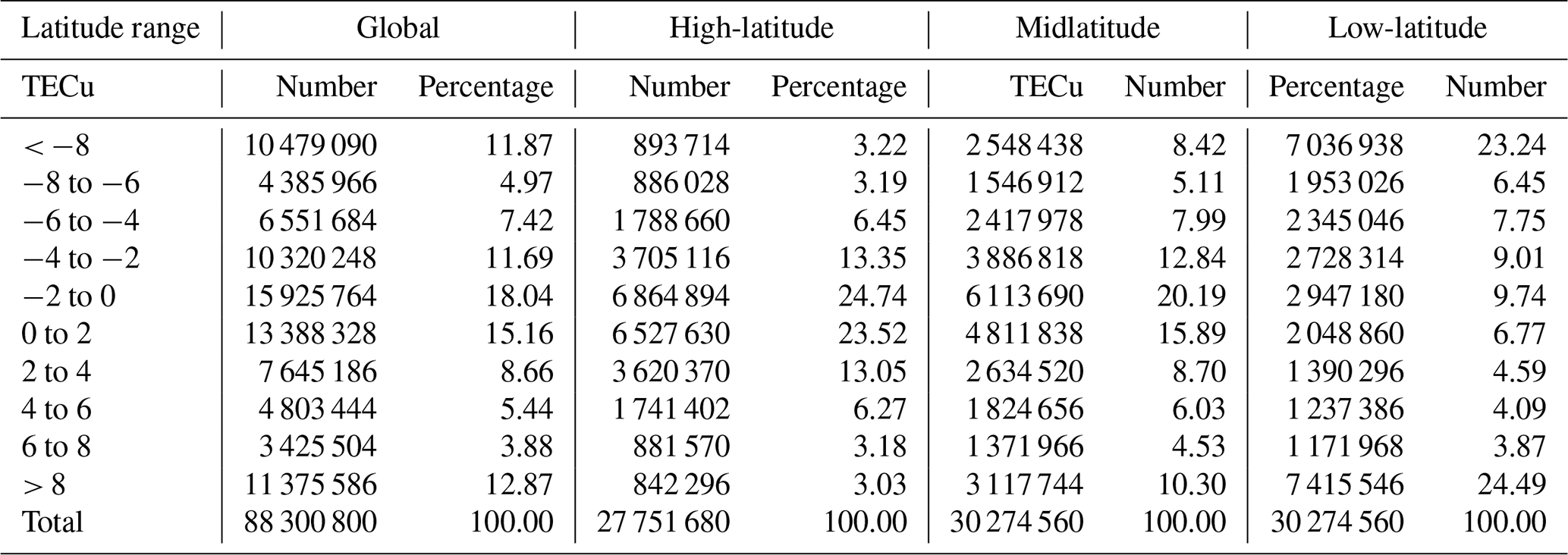
Table 4 Statistics of GIM grid TEC difference in adjacent time in 2021.

3.2 Temporal variation

On the timescale, the adjacent moments of each GIM map are differenced, and there are four differences for each grid. By taking the difference in each grid as a unit, the maximum, mean and minimum values of the absolute values of these differences are counted to analyze the change in TEC of the grid in time, and then the change in TEC of the GIM grid in time for the whole year is counted. It should be noted that, for the sake of data uniformity, all GIMs are counted at 2 h intervals, i.e., 13 frames per day, in 2014 and 25 frames per day at 1 h intervals in 2021. In order to take into account the effect of the latitude of the grid, these results still need to be counted separately for high, medium and low latitudes.

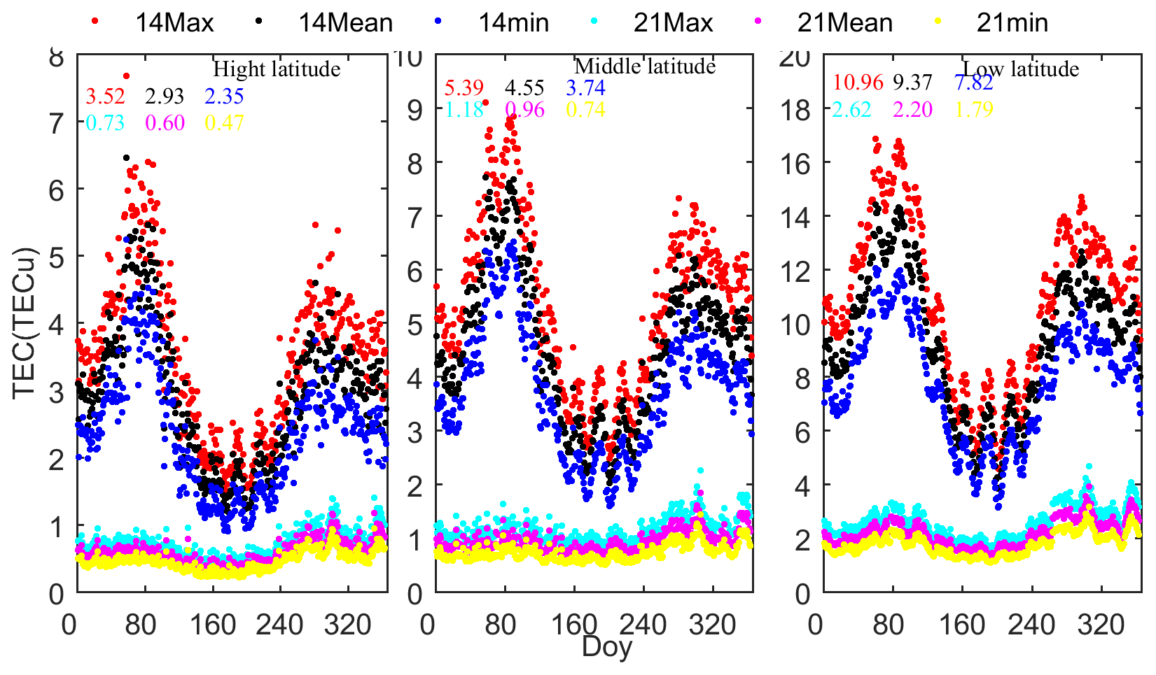
The daily average results of the maximum, average and minimum values of the grid TEC difference between the two GIMs at adjacent moments of each day in 2014 and 2021 are enumerated in Fig. 8. It is obvious from the figure that the variation in the grid TEC difference in 2014 fluctuates greatly, and the trend of the fluctuation is consistent in the three latitudinal regions and the same as the variation in the F10.7 index. It is due to the high solar-activity year and active ionospheric variation in 2014, which conforms to the previous results. Despite the large variation in the grid TEC difference in 2014, it is still evident that the high and middle latitudes are smaller than the low latitudes specifically in terms of values. In contrast, the variation trend of the grid TEC difference in 2021 is relatively gentle and most of the variation values at high and low latitudes are within 2 TECu. On the one hand, this is because 2021 is a low solar-activity year with a flat ionospheric activity. And on the other hand, it is attributed to the GIM time interval of 1 h in 2021, while the interval in 2014 is 2 h.

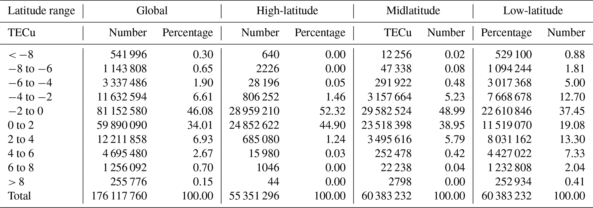
For further analysis, the TEC differences in all adjacent time grids in a year are counted, and there are four differences for each grid. In 2014, all the grids are counted at 2 h intervals on 13 maps a day, and there are $\mathrm{4}\times \mathrm{70}\times \mathrm{72}\times \mathrm{12}\times \mathrm{365}=\mathrm{88}\mathrm{300}\mathrm{800}$ differences; in 2021, the grids are counted at 1 h intervals on 25 maps a day, and there are $\mathrm{4}\times \mathrm{70}\times \mathrm{72}\times \mathrm{24}\times \mathrm{364}=\mathrm{176}\mathrm{117}\mathrm{760}$ differences. As in the previous section, the frequency of grid TEC differences between −8 and 8 TECu at 2 TECu intervals is still counted separately according to high and low latitudes. The statistical results for 2014 and 2021 are introduced in Tables 3 and 4. The histograms of TEC grid differences according to each of the three latitudes are shown in Fig. 9.

As can be seen in Table 3, the results of TEC difference values of the GIM grid at adjacent moments in 2014 are relatively scattered, with only 53.55 % within 4 TECu globally; only 74.66 % of the values in the high-latitude region; a minimum of only 30.11 % in the low-latitude region; and nearly half of the TEC difference values exceeding 8 TECu in the low-latitude region, which is related to the active ionospheric changes during the high solar-activity year of 2014. Table 4 provides the statistical results of TEC difference in the GIM grid in adjacent time periods in 2021. Obviously, when the difference range is within 4 TECu, it accounts for 93.63 % globally, while the percentage of high- and low-latitude regions are 99.92 %, 98.96 % and 82.53 %. In particular, 97.22 % of the TEC difference values in high-latitude regions account for less than 2 TECu.

Figure 9 also gives the histograms of the TEC differences in the adjacent moment grids for the high- and low-latitude regions in 2014 and 2021, respectively. It can be clearly found that they follow a normal distribution, but there are some differences in the ranges of their respective distributions. Furthermore, the distribution of the difference in 2014 has a larger range, especially in the low-latitude region with more than 20 TECu, while for 2021, most of its differences in the high-latitude region are within 2 TECu.

4 Conclusions

By utilizing the GIM data from high solar-activity years (2014) and low solar-activity years (2021) provided by CODE, this paper proposes the grid TEC difference as a way of analyzing TEC variation characteristics within the grid, which is conducive to exploring and analyzing the variation characteristics of the ionosphere TEC in the single-station area. The results show that the TEC difference size within a GIM grid is mainly related to the activity of ionosphere. The value is larger in high solar-activity years and generally small in low solar-activity years, and the value of high-latitude areas is always smaller than that of low-latitude areas. Specifically, in high solar-activity years, most of the GIM grid TEC internal differences are within 4 TECu in high-latitude and midlatitude regions, while only 78.17 % are in low-latitude regions; the grid TEC differences at 2 h intervals are more scattered, and larger differences occur in low-latitude regions. In low solar-activity years, the TEC difference values within a GIM grid are mostly less than 2 TECu, and most of them in the high and middle latitudes are within 1 TECu. The GIM grid TEC difference values within 1 h intervals are mostly less than 4 TECu, and most of them in the high and middle latitudes are within 2 TECu. The main finding of this analysis is that the grid TEC differences are small for most GIM grids, especially in the midlatitudes to high latitudes of low solar years. This means that relevant extraction methods and processes can be simplified when TEC within these GIM grids is needed.

The results of the above analysis can help to understand the ionospheric TEC variation characteristics in the GNSS single-station region (which may be the range of several adjacent grids) and provide a corresponding reference for regional ionospheric modeling. The is especially the case for the high-latitude and midlatitude regions with low solar-activity years. Since the TEC difference within the grid varies less, the TEC processes can be simplified accordingly in terms of GNSS single-frequency ionospheric delay correction, single-station regional ionospheric modeling and code bias estimation, etc. The related validation and analysis need to be further studied.