Statistical comparison of electron precipitation during auroral breakups occurring either near the open–closed field line boundary or in the central part of the auroral oval

Auroral electron precipitation during a substorm exhibits complex spatiotemporal variations which are still not fully understood, especially during the very dynamic phase immediately following the onset. Since during disturbed times, the auroral oval typically extends across several hundreds of kilometres in the latitudinal direction, one may expect that precipitating electron spectra differ at locations close to the open–closed field line boundary (OCB) compared to the central part of the auroral oval. We carry out a statistical study based on 57 auroral breakups associated with substorm onsets observed above Tromsø (66.7° N geomagnetic latitude, i.e. central oval) and 25 onsets occurring above Svalbard (75.4° N geomagnetic latitude, i.e. poleward boundary) between 2015 and 2022. The events were selected based on the availability of both optical observations and field-aligned incoherent scatter radar measurements. Those are two sets of different substorms; hence, we compare solar wind driving conditions and geomagnetic indices for the two event lists in the statistical sense. Using the ELectron SPECtrum (ELSPEC) method (based on the inversion of the electron density profile) on the radar data, we retrieve precipitating electron fluxes within 1–100 keV around each onset time, and we apply the superposed epoch analysis method to the electron spectra at each location. We compare the statistical precipitation characteristics above both sites in terms of the peak differential flux, the energy of the peak, the integrated energy flux, and their time evolution during the minutes following the onset. We find that the integrated energy flux associated with events occurring in the central part of the auroral oval (Tromsø) exhibit a sharp peak of up to 25 mW m⁻² in the first 2 min following the auroral breakup before decreasing and maintaining stable values of around 7 mW m⁻² for at least 20 min. In turn, no initial peak is seen near the open–closed field line boundary (Svalbard), and values remain low throughout (1–2 mW m⁻²). A comparison of the median spectra indicates that the precipitating flux of > 10 keV electrons is lower above Svalbard than above Tromsø by a factor of at least 10, which may partly explain the differences. However, it proves difficult to conclude whether the differences originate from the latitude at which the auroral breakup takes place or from the fact that the breakups seen from Svalbard occur Equatorward from the radar beam, which only sees expansion-phase precipitation after a few minutes.

1 Introduction

A crucial element in the dynamics of the magnetosphere–ionosphere system, the phenomenon called “substorm” is one of the processes during which a significant transfer of energy occurs from the magnetosphere to the ionosphere. A magnetospheric substorm occurs as the result of solar wind driving, typically when the interplanetary magnetic field (IMF) north–south component is oriented southward (B_z<0). It consists of a large-scale and sudden reconfiguration of the magnetotail topology, with highly stretched geomagnetic field lines reconnecting and dipolarising. The result of this dramatic magnetic field reconfiguration is reflected in the ionosphere as an auroral substorm (Akasofu, 1964). The auroral substorm starts with a growth phase, in which an auroral arc gradually drifts Equatorwards. At some point, this arc brightens and becomes active; this is the auroral breakup, followed by the substorm expansion phase, during which the aurora extends across latitudes in the poleward direction. Finally, during the recovery phase, active auroral structures disappear and give way to a large-scale diffuse aurora, which may include a pulsating aurora (e.g. Oyama et al., 2017). The average duration of a substorm is on the order of 2 h, but there is a large variability in this duration (e.g. Partamies et al., 2013).

Substorms are a very common phenomenon: several studies have shown that they occur, on average, several times per day (Borovsky and Yakymenko, 2017), which translates into about 1000 substorms per year (Partamies et al., 2013). As a result, substorms are a basic element in the cycle of energy storage and release from the magnetospheric perspective and in the energy input from the high-latitude ionospheric point of view.

A long-term statistical analysis of the space-borne measurements of particle precipitation during substorms by Wing et al. (2013) showed that the precipitation power increases dramatically at the substorm onset. The precipitation was categorised into diffuse, monoenergetic, and broadband precipitation of electrons and ions, and the three different classes showed an increase in power of 310 %, 71 %, and 170 % at the substorm onset, respectively. In the superposed epoch analysis, the sharp rise in the wave and monoenergetic electron auroral power started about 15 min before the epoch onset, as determined from the global auroral images.

A more detailed view of particle precipitation during substorms can be obtained by looking at the differential fluxes of particles, which are also known as particle spectra. Substorm particle precipitation spectrum has been investigated in about 150 overpasses of Defense Meteorological Satellite Program (DMSP) and/or Polar Operational Environmental Satellites (POES) (Partamies et al., 2021). About 30 overpasses took place during substorm expansion and about 120 overpasses during substorm recovery phases over northern Fennoscandia. These substorm spectra were found to be mostly confined within the spectral boundaries set by an earlier study on electron precipitation during a pulsating aurora (Tesema et al., 2020). During the expansion phase in particular, however, the precipitating electron fluxes at about 1–10 keV were enhanced compared to the pulsating aurora particles, which was taken as a good proxy for a substorm recovery-phase aurora.

Many of the auroral substorm studies focus on events centred at or close to the core latitudes of the auroral oval, around geomagnetic latitudes of 65–70° (e.g. Nishimura et al., 2010). Statistical substorm studies, on the other hand, have often been based on ground magnetic indices (e.g. Tanskanen, 2009; Newell and Gjerloev, 2011; Forsyth et al., 2015) or global satellite data (e.g. Frey et al., 2004; Wing et al., 2013) without specifying the event location. The latter obviously implies that the events are global-scale events and therefore occupy large areas of the auroral oval.

In turn, few high-latitude substorm studies can be found in the literature. Based on substorm observations in ground-based magnetometer data, Singh et al. (2012) concluded that the high-latitude substorms occur during low or moderate solar wind stream, i.e. solar wind driving conditions that are milder than those during substorms at more central oval locations. Cresswell-Moorcock et al. (2013) focused on events of energetic electron precipitation (electrons with energies above 30 keV) without requiring optical observing conditions. Their event detection was based on electron density enhancements in the ionospheric D region, which resulted in stronger solar wind driving conditions, as reported by the authors. Prior to their study, events of strong D-region ionisation during substorms were not expected to reach L values higher than 10 as the source of high-energy electrons is the outer radiation belt, which rarely extends to high latitudes. Their observations of electron density, however, were collected from the EISCAT Svalbard radar at about L=16. It was concluded that in 2006–2010, the average probability of substorms with electron precipitation fluxes over 10⁷ cm⁻² s⁻¹ sr⁻¹ at energies above 30 keV (as measured by particle detectors on POES spacecraft) is 0.4 %, which corresponds to a couple of events per year.

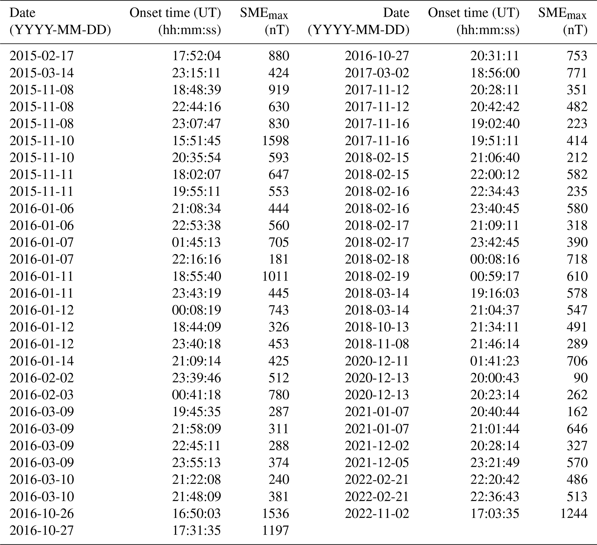
Table 1 List of auroral breakups above Tromsø. SME_max gives the maximum value reached by the SME index in the 20 min following the onset time.

Apart from the abovementioned studies, the high-latitude substorm precipitation in particular has been poorly investigated. High-latitude auroral breakups are expected to be expansions from substorms whose core activity is located in the central auroral oval region at lower latitudes. Another expected class of high-latitude auroral breakups is poleward boundary intensifications (e.g. Nishimura et al., 2021), which are short-term and localised auroral brightening events at the poleward boundary of the auroral oval. However, as demonstrated by the previous high-latitude studies of substorms, there are auroral breakups and substorms at high latitudes, close to the polar cap boundary, that are similar to the substorms and auroral breakups at the central oval latitudes. Setting the terminology aside, the electron precipitation is poorly characterised for these events, partly due to the scarcity of the electron precipitation measurements.

In this paper, our aim is to analyse electron precipitation and compare substorm characteristics over high-latitude and central oval locations. Most previous precipitation studies have used spacecraft measurements, which give a good overview but average transient variations and do not allow one to distinguish between spatial and temporal variability. On the other hand, excellent observations of electron precipitation can be provided by the incoherent scatter radars, which are capable of resolving the ionospheric electron density with high spatial and temporal resolutions above the radar location. Of course, the fixed ground location then makes it challenging to draw conclusions on large-scale dynamical events, such as substorms. Since our goal is to compare local and high-resolution electron precipitation characteristics, such radar measurements are best suited to this study. The paper is organised as follows: Sect. 2 introduces the data and methods used in the study. The results are presented in Sect. 3, which is followed by a discussion in Sect. 4. The main findings of the study are summarised in Sect. 5.

2 Data and methods

We gathered data from EISCAT incoherent scatter radars (ISRs) and auroral all-sky cameras between 1 February 2015 and 31 December 2022. We first searched for clear auroral breakup signatures in the optical data and then checked for suitable radar data availability at the time of those breakups. We performed this operation to obtain lists of events for both Tromsø (central oval; Table 1) and Svalbard (high latitude; Table 2).

2.1 All-sky camera images and auroral breakup detection

The Tromsø optical data come from an all-sky camera, which has been in use in Ramfjordmoen (66.7° corrected geomagnetic latitude) since 2011. The data come from a series of Nikon digital cameras (D5000, D5100, and D7200) that produce an all-sky image every minute (Nanjo et al., 2022). In Tromsø, the aurora season when optical data are available lasts from September to March. Auroral breakups were found using the AI-based aurora classification method developed by Nanjo et al. (2022), whose results are publicly available at https://tromsoe-ai.cei.uec.ac.jp/ (last access: 2 September 2024). We first selected nights where the “discrete” type of aurora was present, with over 90 % probability for consecutive images, indicating auroral activity compatible with one or several substorm onsets during the night. We then inspected the corresponding keogram at the start times of the discrete aurora for whether they were showing a sudden brightening of the aurora associated with a rapid poleward (i.e. northward) motion of the emission source region. A visual inspection of the all-sky images around those candidate events enabled the final selection or rejection of these events as a breakup event and a more accurate determination of the onset time based on the image timestamps. The criterion retained for the breakup starting time was the brightening of an auroral arc, provided that it was shortly followed by a poleward expansion of the optical emission region far enough for it to reach the magnetic zenith (as radar observations are field-aligned for our purposes; see Sect. 2.2).

For Svalbard, we used start times of active aurora periods as a starting point (Partamies et al., 2024). The active aurora labelling was automatically performed for the Sony camera data operated by the University Centre in Svalbard (UNIS) at the Kjell Henriksen Observatory (KHO; 75.4° corrected geomagnetic latitude). Sony is a full-colour mirrorless camera with an all-sky lens taking night sky pictures about every 12 s throughout the auroral season, which lasts from early November to the end of February every winter. The Sony camera was installed in November 2015, which is the reason why we consider events from autumn 2015 onward in this study. For some winter seasons, no AI-based classification of the images was available, so the event search was done by a visual inspection of daily keograms in order to identify potential breakup signatures (brightening and poleward motion). Again, this was followed by a visual check of individual images to validate breakup events and determine their timings as accurately as possible.

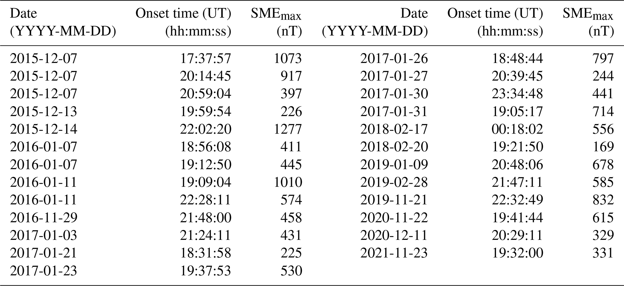
Table 2 List of auroral breakups above Svalbard. SME_max gives the maximum value reached by the SME index in the 20 min following the onset time.

2.2 EISCAT radar data

Once the lists of auroral breakups were established based on the optical data, we checked whether suitable radar observations were available for each event. In this study, we use incoherent scatter radar data from the EISCAT radars located in Ramfjordmoen (Tromsø UHF radar) and Longyearbyen (EISCAT Svalbard Radar, ESR). Measurements from an incoherent scatter radar enable the retrieval of plasma parameters (electron density, electron and ion temperatures, and ion line-of-sight velocity) in the probed ionospheric column. EISCAT radars are typically operated according to a request-based schedule; hence, the radar data are not continuously available, and the experimental setup (pointing direction, pulse code, etc.) varies.

For our purposes, we need specific radar experiment configurations – namely, observations along the geomagnetic field direction. This implies that breakup events occurring during vertical, low-elevation, or scanning-mode EISCAT experiments had to be discarded. In practice, we have considered the following radar experiments: arc1, beata, folke, tau7, ipy, and taro. Ultimately, we obtained a list of 57 breakups above Tromsø and a list of 25 breakups above Svalbard. These lists of retained events are given in Tables 1 and 2, respectively.

The fact that the number of events above Svalbard is significantly lower than that above Tromsø is the result of several factors: (i) the short optical season at such high latitudes (November to February, i.e. 4 months only, whereas the optical season in Tromsø lasts from September to March, i.e. 7 months); (ii) the cloud cover (statistically ∼ 50 % of all image data), which severely reduces the amount of optical observing conditions; (iii) the lower number of substorms occurring at Svalbard latitudes compared to Tromsø latitudes; and (iv) the fact that ESR is operated less often than the EISCAT mainland radars. Since the Sony camera started operating on 4 November 2015, we consider its entire available dataset up to the end of 2022. When using the same time interval for optical data from both locations to sample the same solar activity conditions, this yields 25 events over Svalbard and 57 events over Tromsø.

We use the EISCAT data at the highest available time resolution, which is generally 5 s or 6.4 s, depending on the experiment associated with a given event. In order to obtain good enough of a signal-to-noise ratio at this time resolution, all the EISCAT data have been reanalysed with the Guisdap software (Lehtinen et al., 1996) without fitting the electron and ion temperatures – which are then taken from the International Reference Ionosphere (IRI; Bilitza et al., 2022) model. For our purposes, in this study, we will only consider the electron density. While using the IRI values for the electron and ion temperatures can cause bias in the fitting of electron densities above 115 km in altitude, which also affects the energy spectra fits (Tesfaw et al., 2022), the overall characteristics of the retrieved energy spectra will be sufficiently accurate for the purposes of this study.

2.3 Precipitating electron spectra determination

We apply the ELSPEC (ELectron SPECtrum) method (Virtanen et al., 2018) to the high-resolution EISCAT data to retrieve precipitating electron differential fluxes. ELSPEC is an inversion-based method which enables the retrieval of precipitating electron fluxes in the 1–100 keV energy range based on field-aligned ISR measurements. The lower-energy limit of 1 keV comes from the fact that the inversion of radar data from above 150 km in altitude becomes less reliable due to the significant fraction of O⁺ in the ion content and transport effects. The method consists of analytically integrating the continuity equation and fitting different models of precipitating spectra until the radar observations are best reproduced. The parametric differential number flux model is designed to be able to produce a wide range of spectral shapes, encompassing those that one can expect to observe with the radar. This includes not only simple descriptions, such as Maxwellian distributions, but also more complex and distorted ones, such as kappa distributions. More details on how ELSPEC works can be found in Virtanen et al. (2018).

For each event, we hence obtain the precipitating electron spectra in the radar field of view at the highest available time resolution. Energy bins are logarithmically spaced, and the energy range approximately corresponds to electrons depositing their energy within 80–150 km in altitude in the ionosphere.

Figure 1 gives an example event from Svalbard, which took place on 12 December 2015. The optical observations (Fig. 1a) reveal an auroral breakup around 17:38 UT followed by an expansion phase that brings auroral emissions into the beam of ESR (beam elevation indicated by a dashed white line). Electron density measurements by ESR (Fig. 1b) indicate a sudden enhancement at all E-region altitudes, with a short-lived peak near 120 km in altitude at 17:39 UT and later on electron density increases, peaking within 90–110 km in altitude between 17:47 and 17:55 UT. There is a very clear match between the E-region electron density and auroral brightness evolution at the elevation of the ESR beam. The results of the ELSPEC analysis of this event (Fig. 1c) indicate that ∼ 1–10 keV electron precipitation started to appear within the radar beam around 17:39 UT, producing the aforementioned first electron density increase. Precipitation then continued with lower fluxes until 17:47 UT, which coincides with a new increase in the auroral brightness at the beam elevation (magenta line; in arbitrary units since the Sony camera is not photometrically calibrated). During this phase of the auroral display (17:47–17:55 UT), the retrieved precipitating spectra contain electrons with energies of up to 100 keV, which is consistent with the lower altitude of the E-region electron density peak.

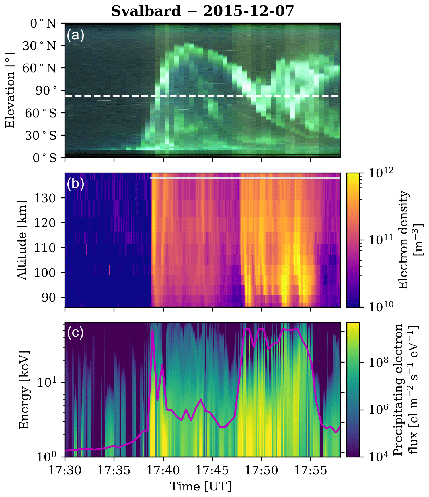
Figure 1 Example of auroral breakup observed above Svalbard on 7 December 2015. (a) Keogram from the Sony camera in Longyearbyen. The dashed white line indicates the elevation corresponding to the local magnetic field direction, i.e. the pointing direction of ESR. (b) Electron density profile measured by ESR. (c) Precipitating electron differential number flux derived with the ELSPEC method from the ESR measurements. The magenta line indicates the optical emission brightness (arbitrary unit, linearly scaled) within the ESR beam, i.e. along the dashed white line in panel (a). The small light-grey dots at the top of panel (b) indicate times with “valid” data points retained in the superposed epoch analysis (see Sect. 3.2) for this event.

2.4 Solar wind driving and geomagnetic conditions

To assess to what extent the two sets of events (Tromsø and Svalbard auroral breakups) are associated with different driving conditions in the statistical sense, we gather solar wind data propagated to the nose of the Earth's bow shock. These data were downloaded from the OMNI database at a 5 min time resolution (King and Papitashvili, 2005; Papitashvili and King, 2020).

We further consider the SuperMAG electrojet index (SME; Newell and Gjerloev, 2011) and the SYM-H index (Wanliss and Showalter, 2006) as measures of substorm activity and geomagnetic activity, respectively. These two geomagnetic indices are calculated from ground-based magnetometer measurements.

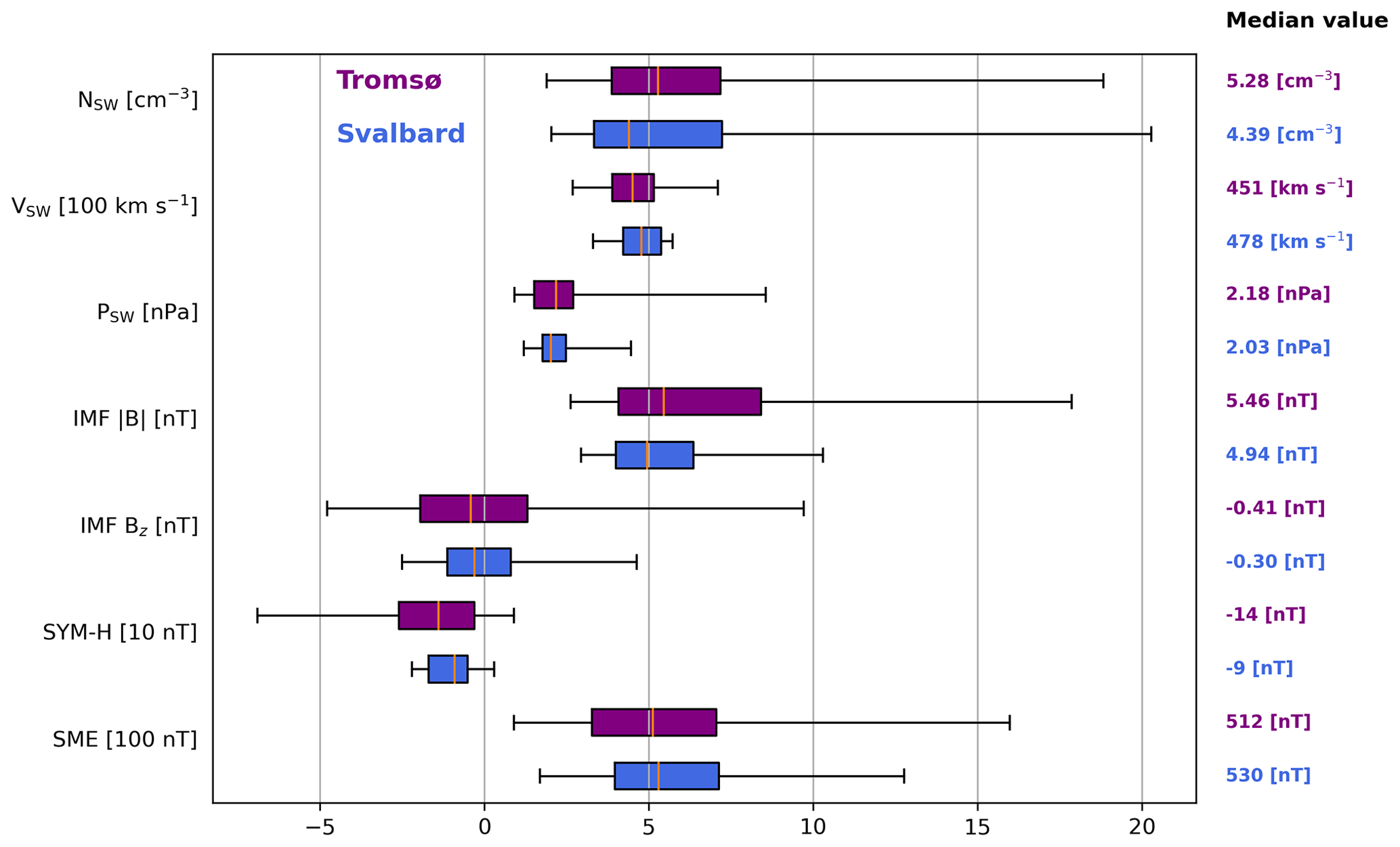
Figure 2 Distribution of driving (solar wind density, speed, and dynamic pressure; IMF magnitude and B_z component) parameter averages during the 2 h preceding each event at Tromsø (TRO) and on Svalbard (LYR). For geomagnetic indices, we give the distribution of their most extreme (minimum for SYM-H, maximum for SME) value during the 20 min following the onset time for each event. Median values of the distributions are given on the right.

3 Results

3.1 Driving conditions during the events

Figure 2 gives the statistical distribution of the solar wind and IMF conditions as well as geomagnetic indices during the Tromsø (data shown in purple) and Svalbard (in blue) auroral breakups. For each solar wind and IMF parameter and each event, we calculate the mean value during the 2 h preceding the auroral breakup (chosen as a compromise to smooth out short-lived variations in the parameters while giving a measure of the conditions prior to the breakups) to assess driving conditions in which the breakup occurs. For the geomagnetic indices, we rather consider the most extreme value (minimum for SYM-H and maximum for SME) during the 20 min following the breakup time to look at the response. We then examine the statistical distributions of these parameter values across events. The boxes indicate the interquartile range, with the median showing as a vertical orange line within the box, and the “whiskers” indicate the full range of values. Median values are in addition indicated to the right of the plot, for each parameter.

It is apparent from the figure that, overall, the driving conditions producing the Tromsø and the Svalbard auroral breakups are not very different, in the statistical sense. Solar wind density, speed and pressure exhibit values showing quite similar medians and dispersion without any consistent trend to separate the Svalbard events from the Tromsø events. Concerning the IMF, the Tromsø events are associated with slightly larger driving than the Svalbard events (although the differences in terms of median values are very small), and the IMF magnitude and B_z values have a larger spread. This dispersion is reflected in the geomagnetic index statistics, with Tromsø events being associated with more dispersed values of SYM-H and SME than Svalbard events. Median behaviours for those two geomagnetic indices are however quite similar to each other, with Tromsø events having a median SYM-H slightly lower than Svalbard events (hence indicating slightly stronger geomagnetic activity), whereas in turn the median SME is slightly lower (indicating a slightly weaker substorm activity). Therefore, the main conclusion from Fig. 2 is that, although the auroral breakups and expansion phases considered in this study consist of different events in the Tromsø and Svalbard lists of events, they are associated with relatively similar average driving (solar wind and IMF) and average geomagnetic responses (SYM-H and SME).

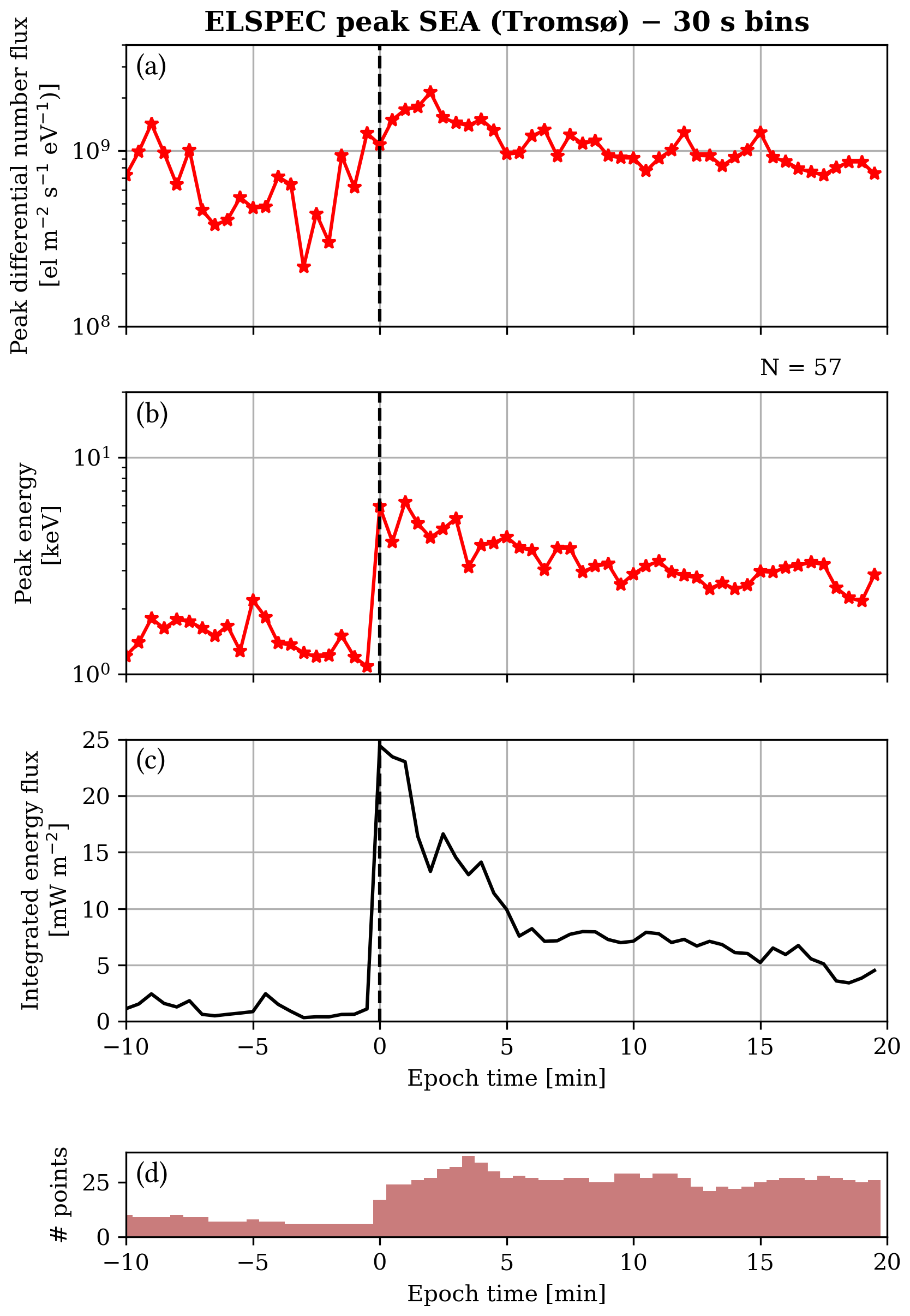
Figure 3 Superposed epoch analysis of the peaks of precipitating spectra obtained with ELSPEC for the Tromsø events. In all panels, the zero epoch corresponds to the auroral breakup as identified in the optical data (Nikon camera in Ramfjordmoen) and the median values are calculated in 30 s bins. (a) Peak differential number flux. (b) Peak energy. (c) Integrated energy flux of auroral electron precipitation. (d) Number of data points with valid values from which the medians are computed in the above panels.

3.2 Precipitation characteristics in Tromsø

To investigate the characteristics of auroral electron precipitation above Tromsø during auroral breakups and expansion phases, we apply the superposed epoch analysis method. We define the zero epoch of each event as the time when the main auroral arc visible in optical data brightens up to later expand poleward (see Sect. 2.1). These are the times given in Table 1.

We first consider the characteristics of the auroral electron precipitation peak in the spectra retrieved by ELSPEC during the events. Figure 3 shows the median values of the peak differential number flux (Fig. 3a) and the corresponding electron energy (Fig. 3b) obtained with the superposed epoch analysis of Tromsø breakups and expansion phases. The given time window starts 10 min before the zero epoch and lasts until 20 min after the zero epoch. We also provide the median value of the integrated energy flux (Fig. 3c).

In this analysis, although the EISCAT (and hence ELSPEC) data have been generated at the highest available time resolution (5 s or 6.4 s depending on the event), we collected them into 30 s bins to improve the signal-to-noise ratio. In practice, for each event, we take the mean of the valid values in every 30 s bin, and this mean value is then the data point associated with this event in the superposed epoch analysis.

To ensure that we only consider data points associated with particle precipitation above EISCAT, we discard those where no significant electron density enhancement compared to the background is observed at auroral emission altitudes. For each event, we first calculate the time series of the median electron density measured by EISCAT across altitudes of between 85 and 125 km (lower E region), $N_e^{\mathrm{85}-\mathrm{125}\mathrm{km}}\left(t\right)$. We then calculate the mean value of this quantity in the 2 min preceding the onset time, $N_e^{\mathrm{bgd}}={〈N_e^{\mathrm{85}-\mathrm{125}\mathrm{km}}\left(t\right)〉}_{t_{\mathrm{0}}-\mathrm{2}\min <t<t_{\mathrm{0}}}$, which we take as the background auroral-altitude value for electron density for the given event. A precipitating electron spectrum is deemed valid for our superposed epoch analysis if the auroral-altitude electron density exceeds this background value by at least a factor of 3 (value determined empirically), i.e. if $N_e^{\mathrm{85}-\mathrm{125}\mathrm{km}}\left(t\right)>\mathrm{3}{N}_e^{\mathrm{bgd}}$. As a result, during a given event, only the times when there was electron precipitation above the radar are retained for the superposed epoch analysis. This avoids systematically underestimating the fluxes following the auroral breakups by introducing data points with no precipitation. To illustrate this, the times corresponding to such valid data points during the 7 December 2015 event above Svalbard are indicated with light-grey dots near the top border of Fig. 1b (forming a grey line). We can see that times prior to the auroral breakup (17:39 UT) do not fulfil the criterion of an enhanced E-region density when compared to the background conditions, whereas almost all times after the auroral breakup are labelled as valid (i.e. have precipitation within the radar beam) for the superposed epoch analysis. It is important to note that the focus on altitudes within 85–125 km is only relevant to this specific step in the analysis (i.e. determining whether there was auroral precipitation in the radar beam at a given time during the event and ignoring the corresponding data point in the superposed epoch analysis if not). The ELSPEC fluxes analysed in the study do encompass energies within the whole range for which the method can be used (1–100 keV), thus leading to electron density enhancements across a broader altitude range than 85–125 km.

Since there are times when no precipitation was taking place within the radar beam (especially before the zero epoch, as expected by the above-described methodology) and since the high-resolution EISCAT data do contain a certain number of invalid values (NaNs) or the ELSPEC analysis occasionally fails to satisfactorily fit a precipitating spectrum, the number of valid data points obtained with ELSPEC is always lower than the total number of events. The number of such valid points associated with each 30 s bin is given in Fig. 3d. Note that whenever a bin contains fewer than three data points, it is excluded from the superposed epoch analysis as the calculated median values of the studied parameters would not at all be statistically meaningful. This does not happen for the Tromsø events shown in this section but becomes important when looking at the Svalbard events in the next section.

The main findings from Fig. 3 can be summarised as follows. The median value of the peak differential number flux (Fig. 3a) during the first 5 min following the auroral breakup is on the order of 2×10⁹ electrons m⁻² s⁻¹ eV⁻¹, after which it slowly decreases to 0.8–1×10⁹ electrons m⁻² s⁻¹ eV⁻¹. Regarding the peak electron energies (Fig. 3b), we obtain median values of ∼ 6 keV immediately after the auroral breakup, which decrease to ∼ 4 keV after 5 min and then stabilise around 3 keV within the 10–20 min time interval. Looking at Fig. 3c, we can see that, at the zero epoch, the median integrated energy flux in Tromsø rapidly changes from < 1 to 25 mW m⁻². It keeps values on this order for about 1 min before decreasing until it reaches a plateau after 5 min of around 7 mW m⁻². We note (Fig. 3d) that throughout the analysed time range after the zero epoch only about half of the events provide data points. This is due to the fact that many observations from the mainland EISCAT radar are carried out with the common programme (CP2) mode, wherein the antenna switches between three pointing directions every few minutes, hence creating gaps in the field-aligned EISCAT dataset that can be analysed with ELSPEC.

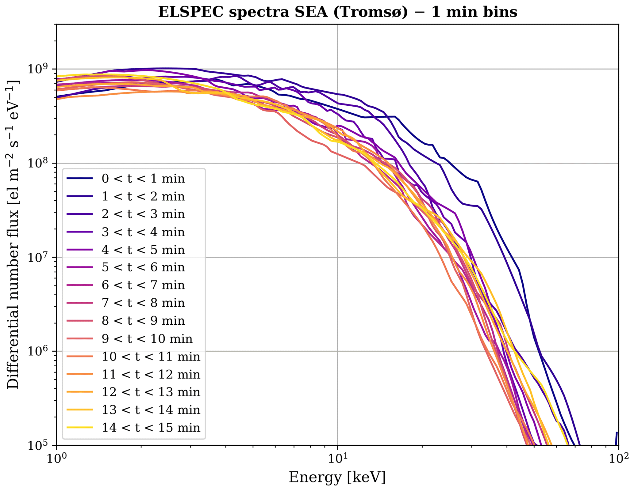
Figure 4 Superposed epoch analysis of the precipitating spectra obtained with ELSPEC from the Tromsø events. The medians of differential number fluxes (i.e. spectra) across events are calculated in 1 min bins after the zero epoch (auroral breakup identified in optical data).

Another way to look at the ELSPEC data is to perform the superposed epoch analysis on the spectra themselves, i.e. by taking the median differential flux value as a function of electron energy during time intervals following the zero epoch (until 15 min after it). The results of this analysis are shown in Fig. 4. Here, we considered 1 min bins and only post-zero-epoch times; the colour of each curve gives the time relative to the zero epoch.

We can see from Fig. 4 that the spectra during the first 2 min following the auroral breakup stand out compared to the curves that correspond to later epoch times. This is especially notable at energies within 20–50 keV, for which those two curves have values 2–5 times greater than the subsequent ones. One can argue that the early curves give median spectra associated with the auroral breakup itself, whereas the late curves represent those associated with the expansion phase. This therefore suggests that the auroral breakup is associated with more energetic electron precipitation than the expansion phase. At $\mathrm{3}<t<\mathrm{15}$ min, the spectra exhibit little variability, with the curves having a dispersion confined within a factor of 3 at most energies. The trend of decreasing peak energy as a function of time following the breakup can be seen during the first 4 min as the peak shifts toward lower energies from the early (blue-shade) curves to the late (pink- and orange-shade) curves. However, with the spectra being relatively flat within the 1–10 keV energy range, the uncertainties associated with the peak energy values are not negligible.

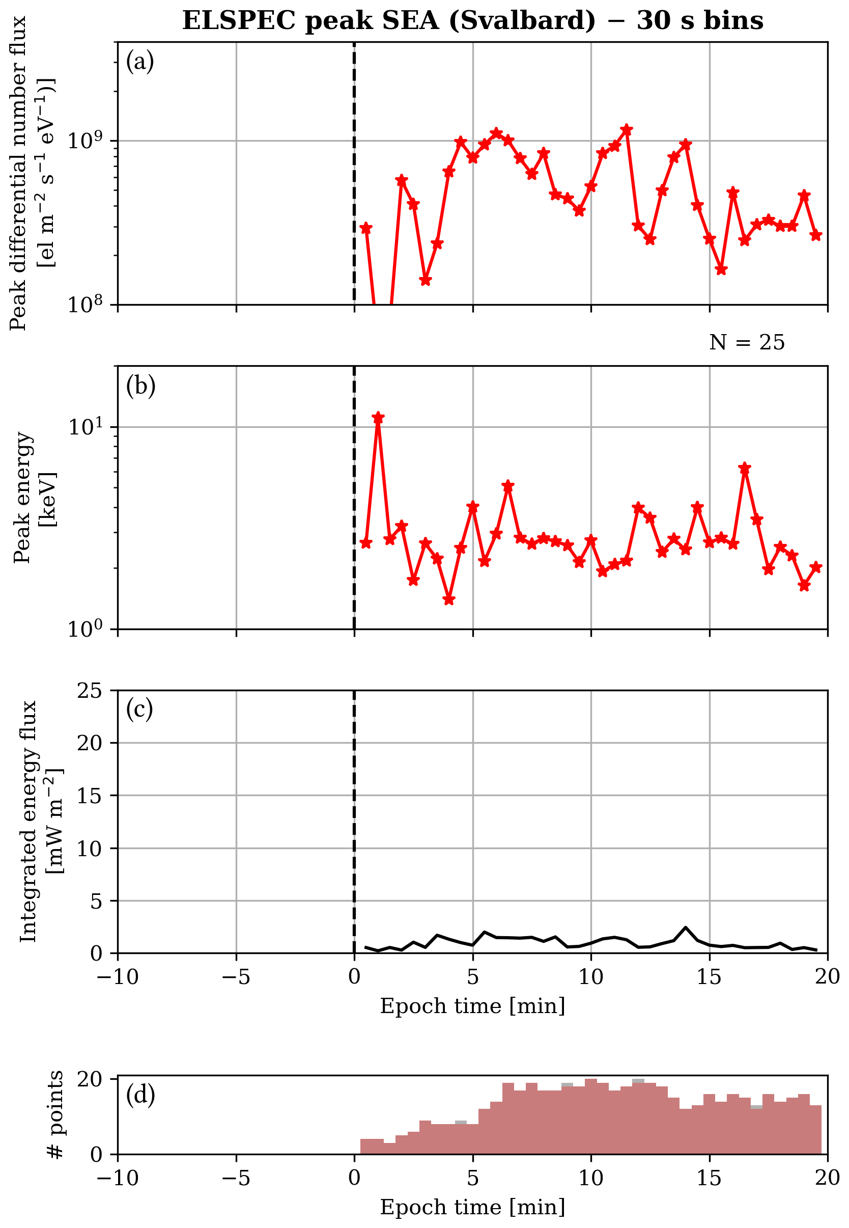
Figure 5 Superposed epoch analysis of the peaks of precipitating spectra obtained with ELSPEC for the Svalbard events. In all panels, the zero epoch corresponds to the auroral breakup as identified in the optical data (Sony camera in Longyearbyen) and the median values are calculated in 30 s bins. The format is the same as in Fig. 3.

3.3 Precipitation characteristics on Svalbard

We apply a similar analysis to the ELSPEC data associated with the Svalbard events. Figure 5 presents the results of the superposed epoch analysis of the characteristics of the spectrum peaks and of the integrated energy flux in the same format as in Fig. 3.

It is clear that almost no precipitation is ever observed before the zero epoch (which corresponds to the auroral breakup time identified in the optical data) as there are never three or more data points out of the 25 events, leading to no median values of the peak parameters and none of the integrated energy flux being calculated. Based on Fig. 5d, we can see that in the first few minutes following the auroral breakup, quite a few (< 10) events have precipitation within the ESR beam: it takes 5 min after the zero epoch for the number of retrieved spectra to be on the order of 15–20 and to provide a robust value for the median. This is likely because Svalbard auroral breakups generally occur Equatorward and/or eastward from the ESR location, meaning that precipitation is detected by the radar only once the aurora has expanded up to the magnetic zenith, which can take a few minutes (as is illustrated in Fig. 1a). This result differs from the situation in Tromsø, where precipitation is detected immediately after the zero epoch.

The peak differential number flux of precipitating auroral electrons retrieved from ESR observations during the Svalbard events reaches 1×10⁹ electrons m⁻² s⁻¹ eV⁻¹ (Fig. 5a). This value is reached during the first 5 min following the auroral breakup (based on the few events where precipitation is retrieved). After that, the peak flux gradually drops until it reaches 3×10⁸ electrons m⁻² s⁻¹ eV⁻¹ after 12–20 min following the zero epoch. Overall, the values within 5–20 min after the zero epoch are 3 to 5 times smaller than the corresponding ones in the Tromsø events.

In terms of peak electron energy (Fig. 5b), apart from an outlier in the first minute after the breakup (unlikely to be very significant given that it is based on only four events), values range within ∼ 2–5 keV and do not appear to vary much during the considered time interval. With the number of events being smaller, the median peak energy time series is noisier for the Svalbard events than for the Tromsø events. We note that, while the values shortly after the auroral breakup are clearly larger from Tromsø than for Svalbard, peak energies are sensibly similar at times greater than 10 min following the zero epoch.

However, a very striking difference between Tromsø events and Svalbard events can be seen in terms of integrated energy flux (Fig. 5c). The integrated energy flux remains very low throughout the studied time interval, with values on the order of 1–2 mW m⁻² most of the time. This is significantly lower (by a factor of 5–10) than the values obtained for the Tromsø events, and there is no apparent maximum at the zero epoch, unlike in Tromsø. The absence of this initial peak is likely due to the fact that ESR misses the auroral breakup and mainly sees the expansion phase, as discussed above. As a last point on this figure, we note that, with such low values for the integrated energy flux, the peak electron energies discussed in the previous paragraph may not be very reliable due to the difficulty in fitting the spectrum shape when the electron density is only mildly enhanced by particle precipitation.

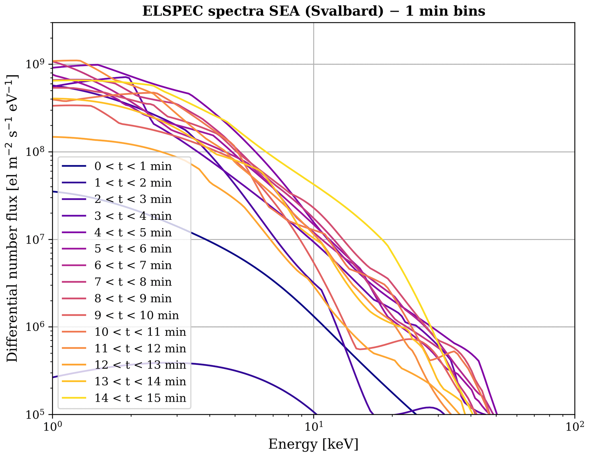
Figure 6 Superposed epoch analysis of the precipitating spectra obtained with ELSPEC from the Svalbard events. The medians of differential number fluxes (i.e. spectra) across events are calculated in 1 min bins after the zero epoch (auroral breakup identified in optical data). The format is the same as in Fig. 4.

Figure 6 sheds some light on the reason for the large discrepancy in integrated energy flux between the Svalbard breakups and the Tromsø breakups. This figure gives the result of the superposed epoch analysis applied to the spectra obtained with ELSPEC for the Svalbard events, compiled in 1 min bins, in the same way as in Fig. 4 for the Tromsø events.

The figure confirms that little precipitation occurs above ESR during the first 2 min following the zero epoch, as the corresponding curves are clearly lower than the others. This is consistent with the fact noted above that auroral breakups seen from Svalbard originally occur slightly outside of the ESR magnetic zenith and that the aurora only reaches the radar beam after a few minutes during the expansion phase. Then, the median spectra all have a similar shape, with the notable exception of the one corresponding to data between 9 and 10 min following the zero epoch, which exhibits a secondary peak at ∼ 25 keV. This secondary peak might be the result of one or a few events with a high-energy peak, which could correspond to monoenergetic (inverted-V) precipitation. In any case, the magnitude of this secondary peak is about 1000 times lower than that of the main peak (at about 1 keV), so its significance is likely minor. We note that the dispersion of differential number flux values corresponds to about a factor of 10 throughout the energy range, which is sensibly larger than the dispersion noted on the curves from Tromsø events. The spectra are relatively flat at low energies; hence, there is no clear peak energy value exhibiting variability as a function of time since the breakup that emerges from this analysis.

A clear difference between Figs. 4 and 6 can be found in the medium range of energies (especially at ∼ 3–30 keV). The median differential number flux values in Tromsø are larger than those in Svalbard by a factor of at least 10. This is the reason why the integrated energy flux in Tromsø is significantly greater than that in Svalbard. Besides, we can see that the slope of the spectra in the high-energy range is steeper in Tromsø than on Svalbard. As a result, the ratio between differential number fluxes in Tromsø and in Svalbard is only on the order of 3–4 at 30 keV energies. However, since precipitating fluxes at these energies have very low values compared to the main peak, the contribution of these electrons to the energy input into the upper atmosphere is relatively small.

4 Discussion

The first interesting result from this study is the absence of a notable difference in terms of driving (solar wind and IMF) and geomagnetic conditions associated with the Svalbard events on the one side and the Tromsø events on the other side. The solar wind driving conditions are overall in good agreement with the results obtained by Singh et al. (2012), who found that high-latitude substorms typically occur during low or moderate solar wind driving conditions (speed of under 500 km s⁻¹). This agreement is found despite using different approaches in selecting events (auroral breakups detected in optical data in our case and substorm onsets identified in ground-based magnetometer data in their case). The fact that our Svalbard events are associated with slightly higher solar wind speed (median value of 478 km s⁻¹) than theirs (median value between 351 and 400 km s⁻¹) is likely because their study considered events that took place during the deep solar minimum of solar cycle 23 (austral summers of years 2007–2010), during which geomagnetic activity was very low (e.g. Grandin et al., 2019). Our events, in turn, took place between 2015 and 2022, which encompasses not only solar minimum years, but also the declining and rising phases of the solar cycle.

While we have identified clear differences between the precipitating electron spectra retrieved during Svalbard auroral breakups compared to those retrieved during Tromsø substorms, the reason behind those contrasts is not straightforward. Our hypothesis A is the question of whether the lower integrated energy flux associated with the Svalbard breakups an inherent characteristic of the high-latitude substorms. Alternatively, hypothesis B begs the question of whether it rather stems from the fact that events observed by ESR generally have their breakups outside the Svalbard magnetic zenith, and precipitation is only observed after some minutes of expansion. In case A, this would mean that the precipitating spectra associated with high-latitude auroral breakups consist of less-energetic electrons compared to those associated with central-oval breakups. This could suggest that precipitation that originates from the outer plasma sheet is less energetic than that originating from the inner plasma sheet. Case B would, in turn, imply that the geomagnetic field lines where the breakup occurs host more energetic precipitating spectra than the field lines where precipitation occurs as the result of the expansion of the aurora. This scenario would be consistent with the result that, during the first 2 min following an auroral breakup above Tromsø, the radar observes a greater integrated energy flux as well as a larger peak differential number flux and peak electron energy than at epoch times within 3–20 min, which are associated with a decreasing trend for all parameters. However, the flux values obtained from Tromsø remain significantly greater than those obtained from Svalbard throughout the studied time interval, which suggests that scenario A may contribute more to the observed differences than scenario B. To be able to investigate this issue in more detail, simultaneous observations of two latitudinally separated geomagnetic field lines during the same set of events would be required.

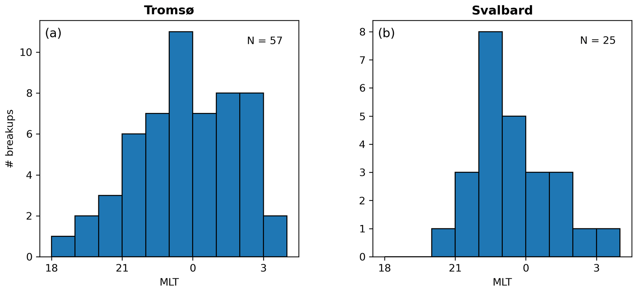
Figure 7 Distribution of the magnetic local times (MLT) at which the events take place above (a) Tromsø and (b) Svalbard.

Another aspect worth checking when comparing the Tromsø events to those from Svalbard is the magnetic local time (MLT) distribution of the auroral breakups. Figure 7 shows the MLT distributions of the listed events for Tromsø (Fig. 7a) and Svalbard (Fig. 7b). We note that the distribution for Tromsø is relatively broad, spanning from 18:00 to 04:00 MLT and having its peak between 23:00 and 00:00 MLT. It is in good agreement with that obtained by (Mende et al., 2023), who studied 91 substorm onsets using global auroral images in the far ultraviolet from the IMAGE spacecraft. In turn, the distribution for Svalbard is somewhat narrower (from 20:00 to 04:00 MLT) and has its peak between 22:00 and 23:00 MLT. More importantly, only a small fraction (8 out of 25) of the Svalbard events come from post-midnight MLTs, contrary to the Tromsø events, for which a comparatively larger fraction (25 out of 57) are associated with post-midnight MLTs. Since previous studies have indicated that precipitating spectra tend to be more energetic in the post-midnight sector (Hosokawa and Ogawa, 2015; Partamies et al., 2017), this could be another contributing factor to the differences in the > 10 keV fluxes retrieved for Svalbard and Tromsø. Moreover, 14 out of the 57 events from Tromsø occur in March or October, which are outside of the optical season on Svalbard (November through February). With those 2 extra months being closer to the equinoxes, this might produce some bias in the precipitating spectra as equinoxes are known to favour stronger events (e.g. Petrinec et al., 2000; Liou et al., 2001; Newell et al., 2013; Tesfaw et al., 2023). However, excluding those 14 equinox events from the Tromsø dataset and carrying out the same superposed epoch analysis do not appear to significantly affect our results (not shown). This suggests that seasonal effects are unlikely to be the explanation for the obtained discrepancies between Svalbard and Tromsø breakups.

One limitation of this study is the relatively low number of events, especially in the Svalbard list of auroral breakups, despite considering 8 years of data. This is due to the optical observations being limited to the dark season, lasting for 4 months, combined with often unfavourable weather statistics, which limits the number of breakups identified in the optical data. In addition, the need for simultaneous radar operations with specific experiments (ELSPEC can only be used with field-aligned measurements) drastically reduces the number of events. Finally, the complex dynamics associated with the auroral expansion phase implies that not every time following the breakup will have precipitation within the radar beam as discrete auroral structures rapidly evolve and cover only a limited part of the sky. As a result, at most times following the zero epoch, only a handful of events provide data points to calculate the median value across events. This is the reason why we only consider median values and do not show more statistical metrics (e.g. interquartile range). Nonetheless, we note that our number of Svalbard events (25) is exactly the same as in the study by Singh et al. (2012), and we find a relatively similar MLT distribution for the onsets, with most events occurring between 21:00 and 02:00 MLT, though in the Singh et al. (2012) study, the peak is between 23:00–00:00 MLT (22:00–23:00 MLT in our case).

While we can less readily compare our results with the Cresswell-Moorcock et al. (2013) study of high-latitude energetic precipitation signature detected at ESR, we note that their events tend to be associated with stronger solar wind and IMF driving than ours (median value of B_z 2 h before the signature on the order of −2 nT in their case compared to −0.30 nT in ours). In their case, the energetic precipitation signatures in ESR data are significant for about 20 min following the zero epoch, which is sensibly longer than for our events (arguably on the order of 10–15 min). Given that the electron density data from ESR show enhancements down to ∼ 80 km in altitude in the Cresswell-Moorcock et al. (2013) superposed epoch analysis, one can infer that the associated precipitating fluxes include contributions from energies above 50 keV, which, during our events, are only marginally present. We can therefore infer that their events, which were detected based on ESR data (while ours are selected from optical data), are associated with stronger geomagnetic activity than ours. One possible contributing factor to this discrepancy is that their data set includes events in the morning sector, which can comparatively skew the hardness of the precipitating spectra, as underlined above. In addition, since their list of events also includes substorms detected during Northern Hemisphere summer (which our study does not include as it is outside of the optical season), the precipitating fluxes needed to produce a detectable electron density enhancement in the ESR data are comparatively larger given that the background ionosphere is then illuminated by the Sun and hence has a greater electron content. This can be another source of discrepancy in the results, skewing the event selection to stronger driving and geomagnetic activity conditions.

It is worth mentioning that the ELSPEC method provides electron precipitation fluxes of up to 100 keV, but electrons of higher energies can also be present in the precipitation occurring during auroral breakups. Using particle measurements from the Arase satellite in an event study above the Syowa Station in Antarctica (−70.5° geomagnetic latitude, i.e. near the central oval), Kataoka et al. (2019) found that the flux >100 keV electrons showed a sharp increase during the auroral breakup and led to ionisation down to 65–70 km in the mesosphere. Earlier studies evidenced an increase in energetic particle fluxes during substorm onset in the equatorial plane of the inner magnetosphere, causing precipitation in the middle atmosphere (e.g. Kremser et al., 1982).

While in our study we cannot investigate >100 keV electron precipitation, we do get, thanks to ELSPEC, a good measure of the precipitating fluxes at auroral energies (1–100 keV). Virtanen et al. (2018) evaluated the uncertainties in the retrieved spectra and demonstrated that (i) the integral energy flux is always very accurate, even if the spectrum shape is not reproduced exactly; (ii) the integral number fluxes may be noisy in the presence of double-peak structures, but there is no systematic bias; (iii) the peak energies, as defined as the peak of the differential energy flux, reproduce the stronger peak accurately if the spectrum contains two peaks and one of them is clearly stronger than the other; (iv) the peaks having about equal amplitudes in the differential energy flux means that both of them are reproduced reasonably well. In our study, we examine differential number fluxes instead of differential energy fluxes and show the peak amplitudes and energies accordingly, leading to minor differences, but the results regarding the confidence that can be placed in the peak characteristics remain valid. Occasionally, the retrieved spectra do exhibit a double-peaked structure, in which case there may be some level of uncertainty in the obtained spectrum shapes (yet the integrated energy fluxes remain reliable, as mentioned above). Nevertheless, since many spectra are processed together to obtain the 1 min medians over tens of events (Figs. 4 and 6), the effects of secondary peaks are expected to be limited to introducing small ripples in the overall shape of the spectra.

Nonetheless, to the best of our knowledge, this study is the first one to provide a quantitative comparison of auroral-energy precipitating electron fluxes at the poleward edge and in the central part of the auroral oval. Tesema et al. (2020) investigated a large number of events over Fennoscandia (hence in the central and Equatorward parts of the oval) using data from multiple satellites, but their focus was on pulsating aurora, which is a feature of substorm recovery phases. Therefore, our results cannot be readily compared to theirs.

5 Conclusions

We carried out a statistical study of auroral (1–100 keV) electron precipitation during auroral breakup and expansion phases when the breakup takes place in the central nightside auroral oval (Tromsø, 57 events) or near the open–closed field line boundary (Svalbard, 25 events). The considered time frame is the same for both lists of events (2015–2022), but the two sets of events are disjointed.

The main conclusions of this study can be summarised as follows:

1. The solar wind and IMF driving conditions during which the auroral breakups considered in this study took place do not exhibit significant differences between the Svalbard events and the Tromsø events. Geomagnetic activity as measured by the SYM-H and SME indices also does not show large differences between the two sets of events.

2. The auroral breakups from the Svalbard list of events generally take place Equatorward from the ESR location, and very few precipitating fluxes are retrieved in the first few minutes following the breakup. In turn, in Tromsø, a high enough number of events to statistically look at the precipitating spectra have precipitation within the EISCAT UHF beam immediately following the auroral breakup.

3. The precipitating electron differential number flux peaks above Tromsø reach values 3 to 5 times larger than those above Svalbard, especially at times within 5–20 min following the auroral breakup.

4. The precipitating spectra above Tromsø have their peaks at about 7 keV at the time of the auroral breakup and then decrease to about 3 keV. This latter value remains stable during the time interval between 10 and 20 min following the breakup and is quite similar to the energy associated with the peak for the Svalbard events.

5. The median differential number fluxes (spectra) in Tromsø exhibit much less dispersion than the Svalbard ones. This may partly be due to the better statistics given by the larger number of events in the Tromsø auroral breakup list compared to the Svalbard one, yet this might also reveal that auroral breakups occurring in the poleward part of the auroral oval exhibit more variability than those occurring in its central part.

6. The integrated energy flux during the auroral breakup and expansion phase is significantly greater for the Tromsø events (initial peak of 25 mW m⁻², with values around 7 mW m⁻² afterwards) than for the Svalbard events (values barely exceeding 1 mW m⁻²). This is related to the fact that the Tromsø spectra have at least 10 times larger differential number flux values than the Svalbard spectra in the 3–30 keV range.

7. The Tromsø observations suggest that the precipitating spectra contain higher fluxes of > 10 keV electrons during the breakup phase than during the expansion phase. This might partly explain the lower fluxes (especially in terms of integrated energy flux) retrieved for the Svalbard events compared to the Tromsø events since the former typically have their breakup occurring Equatorward from the ESR field of view, and only expansion-phase fluxes are seen by the radar. Nevertheless, these data alone are not sufficient to make a conclusion as those differences might also be due to the latitude at which the auroral breakup takes place (open–closed field line boundary vs. central nightside auroral oval).

To be able to address the open question left by the latest point, one would need to be able to simultaneously retrieve the precipitating spectra both in the auroral breakup region and poleward from it during the expansion phase. While this is not possible with the current radar capability as each radar can only observe along one geomagnetic field line at a given time, EISCAT_3D (McCrea et al., 2015) may bring such opportunities in the near future thanks to its upcoming volumetric observations of the central-oval ionosphere.