F-region drift current and magnetic perturbation distribution by the X-wave heating ionosphere

We present a theoretical and numerical study of the drift current and magnetic perturbation model in the ionosphere by incorporating the ohmic heating model and the magnetohydrodynamic (MHD) momentum equation. Based on these equations, the ionospheric electron temperature and drift current are investigated. The results indicate that the maximum change in electron temperature ΔT_e is about 570 K, and the ratio is $\mathrm{\Delta }{T}_{\mathrm{e}}/T_{\mathrm{e}}$ ∼ 48 %. The maximum drift current density is $\mathrm{8}\times {\mathrm{10}}^{-\mathrm{10}}$ A m⁻², and its surface integral is 5.76 A. Diamagnetic drift current is the main form of current. The low collision frequency between charged particles and neutral particles has little effect on the current, and the collision frequency of electrons and ions is independent of the drift current. The current density profile is a flow ring. We present the effective conductivity as a function of the angle between the geomagnetic field and the radio wave; the model explains why the radiation efficiency was strongest when the X wave is heating along the magnetic dip angle, as reported in recent observations by Kotik et al. (2013). We calculate the magnetic field variation in the heating region based on the MHD theory: the results show that the maximum magnetic field perturbation in the heating area is 48 pT.

1 Introduction

Extremely low-frequency (ELF) waves have irreplaceable advantages in communication, navigation, and magnetospheric studies. In the 1970s, Willis and Davis (1973) first proposed the theory of modulating the ionosphere to excite ELF waves. Then, Getmantsev et al. (1974) successfully excited ELF signals in experiments.

There are several main physical mechanisms of ELF signal excitation by heating the ionosphere. The first mechanism is called the polar electrojet (PEJ) model. A polar electrojet is a strong horizontal electric current driven by an atmospheric dynamoelectric field and a magnetospheric electric field. It can be effectively modulated by heating the ionosphere with a modulated high-frequency (HF) wave. The resulting modification of the electrojet current creates an effective antenna radiating at the modulation frequency (Stubbe et al., 1981; Stubbe and Kopka, 1977; Rietveld et al., 1987). Numerous researchers have analyzed this process theoretically and experimentally and proposed optimization measures such as preheating (Milikh and Papadopoulos, 2007), geometric modulation (Cohen et al., 2008, 2009), and beam painting (Papadopoulos et al., 1990) to enhance the radiation signal. The shortcoming of the PEJ is that the electric field changes suddenly and is difficult to predict (Belyaev et al., 1987). The second mechanism is beat-wave (BW) modulation (Yang et al., 2019). BW modulation can excite ELF waves by dividing the heating source into two groups (Ganguly, 1986; Kuo et al., 2012), in which one group transmits a continuous wave at a frequency f₀ and the other group transmits a continuous wave at a frequency f₀±f (f is the ELF/VLF – very-low-frequency) modulation frequency). Barr and Stubbe (1997) utilized this mechanism to excite 565 and 2005 Hz signals at Tromsø. They thought the BW mode could be approximately equivalent to the beat-wave amplitude-modulated (AM) mode, which may be affected by the natural current intensity. However, Kuo et al. (2010, 2012, 2011) proposed that BW modulation can excite another electrojet-independent ELF/VLF signal which is driven by the ponderomotive force.

Papadopoulos et al. (2011a) proposed an ionospheric current drive (ICD) model based on the experimental results of the High Frequency Active Auroral Research Program (HAARP). Papadopoulos et al. (2011b) proposed that the ELF current is driven in a two-step process based on the model of Lysak (1997). The idea is that HF heating creates a pressure gradient in the heated region, then leading to a diamagnetic current that excites a hydromagnetic wave with the modulation frequency. Kotik et al. (2015, 2013) verified the mechanism experimentally in SURA. They discussed the effects of HF emission frequency, emission direction, and magnetic field activity on radiation signals. Eliasson et al. (2012) established the propagation model of ELF waves in the polar region based on the Hall magnetohydrodynamic (MHD) model. Sharma et al. (2016) extended the radiation propagation model at mid and low latitudes. Mahmoudian and Kalaee (2019) demonstrated that the VLF signal may not penetrate the D region as efficiently as the ELF signal.

At present, theoretical research on ICD theory focuses mainly on the propagation process of an ELF wave. In this paper, considering the effect of transmitter parameters and ionospheric parameters, we develop the ionospheric drift current and magnetic perturbation model by coupling the ohmic heating and MHD momentum equations. We then study the drift current properties and the effects of collisions and transmitter angles on the drift current, and we calculate the magnetic field variation in the heating region.

This paper is organized as follows. In Sect. 2, we give the ohmic heating model for tensor conductivity and derive a formula for the ionospheric drift current using the MHD momentum equation. In Sect. 3, numerical solutions of the model are presented for realistic ionospheric profiles, drift current properties are discussed, and the effect of the emission angle is analyzed. Finally, in Sect. 4, the conclusions are presented.

2 Theoretical model

2.1 HF heating model

The background ionospheric data used in this work are obtained from the HAARP (magnetic inclination 75^∘). Referring to the previous literature (Papadopoulos et al., 2011b), the magnetic field inclination is assumed to be 90^∘. The heating model is simplified to a two-dimensional plane in which the z axis is parallel to the geomagnetic field and the x axis is perpendicular to the magnetic field. The ohmic heating equation is (Shoucri et al., 1984; Löfås et al., 2009)

$$\begin{array}{}\text{(1)}& {\displaystyle \frac{\mathrm{3}}{\mathrm{2}}}{k}_{\mathrm{B}}{N}_{\mathrm{e}}{\displaystyle \frac{\partial T_{\mathrm{e}}}{\partial t}}=\mathrm{\nabla }\cdot (\stackrel{\mathrm{‾}}{\stackrel{\mathrm{‾}}{K_{\mathrm{e}}}}\cdot \mathrm{\nabla }{T}_{\mathrm{e}})+Q_{\mathrm{HF}}+Q_{\mathrm{0}}-L_{\mathrm{e}}(T_{\mathrm{e}},T_{\mathrm{0}}),\end{array}$$

where k_B is Boltzmann's constant, N_e is the electron density, T_e is the electron temperature, Q₀ is the background power source, Q_HF is the ohmic heating by high-power radio waves, L_e(T_e,T₀) is the rate of energy loss due to both elastic and inelastic collisions with ions and neutral particles, and $\stackrel{\mathrm{‾}}{\stackrel{\mathrm{‾}}{K_{\mathrm{e}}}}$ is the thermal conductivity tensor which comes from Banks and Kocharts (1973):

$$\begin{array}{}\text{(2)}& {\displaystyle }\stackrel{\mathrm{‾}}{\stackrel{\mathrm{‾}}{K_{\mathrm{e}}}}=\left(\begin{array}{ccc}\mathrm{0}& \mathrm{0}& \mathrm{0}\\ \mathrm{0}& \mathrm{0}& \mathrm{0}\\ \mathrm{0}& \mathrm{0}& K_{\mathrm{e}\mathrm{0}}\end{array}\right),\text{(3)}& {\displaystyle }{K}_{\mathrm{e}\mathrm{0}}={\displaystyle \frac{\mathrm{7.7}\times {\mathrm{10}}^{\mathrm{5}}{T}_{\mathrm{e}}^{\mathrm{5}/\mathrm{2}}}{\mathrm{1}+\mathrm{3.22}\times {\mathrm{10}}^{\mathrm{4}}(T_{\mathrm{e}}^{\mathrm{2}}/N_{\mathrm{e}})\sum _n{N}_n{Q}_D}},\end{array}$$

where N_n is the density of neutral particles of species n and Q_D is the average momentum transfer cross section, which is calculated by Schunk and Nagy (2009). Q_HF is calculated from Joule heating:

$$\begin{array}{}\text{(4)}& Q_{\mathrm{HF}}={\displaystyle \frac{\mathrm{1}}{\mathrm{2}}}Re\left[{\mathit{E}}^{\ast }\cdot \stackrel{\mathrm{‾}}{\stackrel{\mathrm{‾}}{\mathit{\sigma }}}\cdot \mathit{E}\right],\end{array}$$

where $\stackrel{\mathrm{‾}}{\stackrel{\mathrm{‾}}{\mathit{\sigma }}}$ is the conductivity tensor (Gurevich, 2012):

$$\begin{array}{}\text{(5)}& {\displaystyle }\stackrel{\mathrm{‾}}{\stackrel{\mathrm{‾}}{\mathit{\sigma }}}=\left(\begin{array}{ccc}{\mathit{\sigma }}_{xx}& {\mathit{\sigma }}_{xy}& {\mathit{\sigma }}_{xz}\\ {\mathit{\sigma }}_{yx}& {\mathit{\sigma }}_{yy}& {\mathit{\sigma }}_{yz}\\ {\mathit{\sigma }}_{zx}& {\mathit{\sigma }}_{zy}& {\mathit{\sigma }}_{zz}\end{array}\right),\text{(6)}& {\displaystyle }\begin{array}{rl}& {\mathit{\sigma }}_{xx}={\mathit{\sigma }}_{yy}\\ & ={\displaystyle \frac{{\mathit{\epsilon }}_{\mathrm{0}}{\mathit{\omega }}_{\mathrm{pe}}^{\mathrm{2}}{v}_{\mathrm{e}}}{\mathrm{2}}}\left[{\displaystyle \frac{\mathrm{1}}{(\mathit{\omega }-{\mathit{\omega }}_{\mathrm{ce}}{)}^{\mathrm{2}}+v_{\mathrm{e}}^{\mathrm{2}}}}+{\displaystyle \frac{\mathrm{1}}{(\mathit{\omega }+{\mathit{\omega }}_{\mathrm{ce}}{)}^{\mathrm{2}}+v_{\mathrm{e}}^{\mathrm{2}}}}\right],\\ & {\mathit{\sigma }}_{xy}=-{\mathit{\sigma }}_{yx}\\ & =-i{\displaystyle \frac{{\mathit{\epsilon }}_{\mathrm{0}}{\mathit{\omega }}_{\mathrm{pe}}^{\mathrm{2}}{v}_{\mathrm{e}}}{\mathrm{2}}}\left[{\displaystyle \frac{\mathrm{1}}{(\mathit{\omega }-{\mathit{\omega }}_{\mathrm{ce}}{)}^{\mathrm{2}}+v_{\mathrm{e}}^{\mathrm{2}}}}-{\displaystyle \frac{\mathrm{1}}{(\mathit{\omega }+{\mathit{\omega }}_{\mathrm{ce}}{)}^{\mathrm{2}}+v_{\mathrm{e}}^{\mathrm{2}}}}\right],\\ & {\mathit{\sigma }}_{zz}={\displaystyle \frac{{\mathit{\epsilon }}_{\mathrm{0}}{\mathit{\omega }}_{\mathrm{pe}}^{\mathrm{2}}{v}_{\mathrm{e}}}{{\mathit{\omega }}^{\mathrm{2}}+v_{\mathrm{e}}^{\mathrm{2}}}},\\ & {\mathit{\sigma }}_{xz}={\mathit{\sigma }}_{zx}={\mathit{\sigma }}_{yz}={\mathit{\sigma }}_{zy}=\mathrm{0},\end{array}\end{array}$$

where ε₀ is the vacuum dielectric constant; ω, ω_pe, ω_ce, and v_e are, respectively, the frequency of the incident wave, the ionospheric frequency, the cyclotron frequency, and the frequency of electron collision with other particles; E is the incident electric field; and the incident wave is generally an X wave or an O wave:

$$\begin{array}{}\text{(7)}& \begin{array}{ll}{\mathit{E}}_{\mathrm{X}}=E_{\mathrm{0}}\left(s\right)\sin \left(\mathit{\theta }\right)\widehat{x}+i{E}_{\mathrm{0}}\left(s\right)\widehat{y}& \\ +E_{\mathrm{0}}\left(s\right)\cos \left(\mathit{\theta }\right)\widehat{z},& \mathrm{X}\mathrm{wave},\\ {\mathit{E}}_{\mathrm{O}}=E_{\mathrm{0}}\left(s\right)\sin \left(\mathit{\theta }\right)\widehat{x}-i{E}_{\mathrm{0}}\left(s\right)\widehat{y}& \\ +E_{\mathrm{0}}\left(s\right)\cos \left(\mathit{\theta }\right)\widehat{z},& \mathrm{O}\mathrm{wave},\end{array}\end{array}$$

where θ is the angle between the incident wave and the z axis and E₀(s) is the electric field intensity in the ionosphere (Gustavsson et al., 2010):

$$\begin{array}{}\text{(8)}& E_{\mathrm{0}}\left(s\right)=E\left(s_{\mathrm{0}}\right)\left({\displaystyle \frac{s_{\mathrm{0}}}{s}}\right){\left[{\displaystyle \frac{\mathit{\epsilon }\left(s_{\mathrm{0}}\right)}{\mathit{\epsilon }\left(s\right)}}\right]}^{\mathrm{0.25}}\exp \left(i{k}_{\mathrm{0}}\underset{s_{\mathrm{0}}}{\overset{s}{\int }}N\left(s\right)\mathrm{d}s\right),\end{array}$$

where s is the coordinate along the propagation direction of the wave, ε(s) is the relative dielectric constant, N(s) is the refractive index of the wave in the ionosphere, and the electric field amplitude E(s₀) is estimated by an empirical formula:

$$\begin{array}{}\text{(9)}& E\left(s_{\mathrm{0}}\right)={\displaystyle \frac{\sqrt{\mathrm{30}{P}_{\mathrm{ER}}}}{s_{\mathrm{0}}}},\end{array}$$

where P_ER is the effective radiated power of the transmitter. L_e(T_e,T₀) is the electron cooling rate, which depends mainly on the elastic electron–ion collisions, the elastic electron–neutron collisions, the rotational and vibrational excitation of N₂ and O₂, and the fine-structure excitation of O (Moore, 2007).

2.2 Ionospheric drift current model

In this paper, we think there is no drift current in the magnetic field direction because of the ionospheric electric neutrality (Chen, 2012). We mainly consider the current induced perpendicularly to the magnetic field and ignore the current parallel to the field. In order to simplify the calculation, the positive ion is set as a single O⁺ ion, and the collision between electrons and ions ν_ei, electrons and neutral particles ν_en, and ions and neutral particles ν_in are considered. The influence of neutral wind is ignored. The momentum equation can be written.

$$\begin{array}{}\text{(10)}& {\displaystyle }\begin{array}{rl}m{\displaystyle \frac{\mathrm{d}{\mathit{V}}_{\mathrm{e}\perp }}{\mathrm{d}t}}& =-e\mathit{E}-e{\mathit{V}}_{\mathrm{e}\perp }\times \mathit{B}-{\displaystyle \frac{{\mathrm{\nabla }}_{\perp }{P}_{\mathrm{e}}}{N_{\mathrm{e}}}}\\ & -m{v}_{\mathrm{en}}{\mathit{V}}_{\mathrm{e}\perp }-m{v}_{\mathrm{ei}}({\mathit{V}}_{\mathrm{e}\perp }-{\mathit{V}}_{\mathrm{i}\perp })\end{array}\text{(11)}& {\displaystyle }\begin{array}{rl}M{\displaystyle \frac{\mathrm{d}{\mathit{V}}_{\mathrm{i}\perp }}{\mathrm{d}t}}& =e\mathit{E}+e{\mathit{V}}_{\mathrm{i}\perp }\times \mathit{B}-M{v}_{\mathrm{in}}{\mathit{V}}_{\mathrm{i}\perp }\\ & +m{v}_{\mathrm{ei}}({\mathit{V}}_{\mathrm{e}\perp }-{\mathit{V}}_{\mathrm{i}\perp })\end{array}\end{array}$$

In this work, we focus on the steady state. Therefore, the left-hand sides of Eqs. (10) and (11) are ignored. The electric force can also be ignored since this paper focuses on low frequency. The current can be expressed as

$$\begin{array}{}\text{(12)}& J_{\perp }=N_{\mathrm{e}}e({\mathit{V}}_{\mathrm{i}\perp }-{\mathit{V}}_{\mathrm{e}\perp }).\end{array}$$

Solving Eqs. (10), (11), and (12), we get

$$\begin{array}{}\text{(13)}& J_x=e{\displaystyle \frac{\begin{array}{c}{\mathrm{\nabla }}_{\perp }{P}_{\mathrm{e}}\left(m{\mathit{\nu }}_{\mathrm{en}}+M{\mathit{\nu }}_{\mathrm{in}}\right)\\ \cdot \left(M{\mathit{\nu }}_{\mathrm{ei}}{\mathit{\nu }}_{\mathrm{in}}+m{\mathit{\omega }}_{\mathrm{ce}}^{\mathrm{2}}\right)\end{array}}{\begin{array}{c}m({\mathit{\nu }}_{\mathrm{ei}}^{\mathrm{2}}{\left(m{\mathit{\nu }}_{\mathrm{en}}+M{\mathit{\nu }}_{\mathrm{in}}\right)}^{\mathrm{2}}\\ +m\left(m{\mathit{\nu }}_{\mathrm{en}}\left(\mathrm{2}{\mathit{\nu }}_{\mathrm{ei}}+{\mathit{\nu }}_{\mathrm{en}}\right)+\mathrm{2}M{\mathit{\nu }}_{\mathrm{ei}}{\mathit{\nu }}_{\mathrm{in}}\right){\mathit{\omega }}_{\mathrm{ce}}^{\mathrm{2}}+m^{\mathrm{2}}{\mathit{\omega }}_{\mathrm{ce}}^{\mathrm{4}})\end{array}}},\end{array}$$

$$\begin{array}{}\text{(14)}& J_y=-e{\displaystyle \frac{\begin{array}{c}{\mathrm{\nabla }}_{\perp }{P}_{\mathrm{e}}{\mathit{\omega }}_{\mathrm{ce}}\left(M\right({\mathit{\nu }}_{\mathrm{ei}}-{\mathit{\nu }}_{\mathrm{en}}){\mathit{\nu }}_{\mathrm{in}}\\ +m({\mathit{\nu }}_{\mathrm{in}}{\mathit{\nu }}_{\mathrm{en}}+{\mathit{\omega }}_{\mathrm{ce}}^{\mathrm{2}}))\end{array}}{\begin{array}{c}{\mathit{\nu }}_{\mathrm{ei}}^{\mathrm{2}}(m{\mathit{\nu }}_{\mathrm{en}}+M{\mathit{\nu }}_{\mathrm{in}}{)}^{\mathrm{2}}\\ +m\left(m{\mathit{\nu }}_{\mathrm{en}}\right(\mathrm{2}{\mathit{\nu }}_{\mathrm{ei}}+{\mathit{\nu }}_{\mathrm{en}})+\mathrm{2}M{\mathit{\nu }}_{\mathrm{ei}}{\mathit{\nu }}_{\mathrm{in}}){\mathit{\omega }}_{\mathrm{ce}}^{\mathrm{2}}+m^{\mathrm{2}}{\mathit{\omega }}_{\mathrm{ce}}^{\mathrm{4}}\end{array}}},\end{array}$$

where

$$\begin{array}{}\text{(15)}& {\displaystyle }\begin{array}{rl}{v}_{\mathrm{en}}& =\mathrm{2.33}\times {\mathrm{10}}^{-\mathrm{17}}{N}_{{\mathrm{N}}_{\mathrm{2}}}(\mathrm{1}-\mathrm{1.21}\times {\mathrm{10}}^{-\mathrm{4}}{T}_{\mathrm{e}})T_{\mathrm{e}}\\ & +\mathrm{2.65}\times {\mathrm{10}}^{-\mathrm{16}}{N}_{\mathrm{O}}{T}_{\mathrm{e}}^{\mathrm{0.5}}\\ & +\mathrm{1.82}\times {\mathrm{10}}^{-\mathrm{16}}{N}_{{\mathrm{O}}_{\mathrm{2}}}(\mathrm{1}+\mathrm{0.036}{T}_{\mathrm{e}}^{\mathrm{0.5}})T_{\mathrm{e}}^{\mathrm{0.5}},\end{array}\text{(16)}& {\displaystyle }{v}_{\mathrm{ei}}=\mathrm{5.4}\times {\mathrm{10}}^{-\mathrm{5}}{N}_{\mathrm{e}}/T_{\mathrm{e}}^{\mathrm{1.5}},\text{(17)}& {\displaystyle }\begin{array}{rl}{v}_{\mathrm{in}}& =\mathrm{6.64}\times {\mathrm{10}}^{-\mathrm{16}}n\left({\mathrm{O}}_{\mathrm{2}}\right)\\ & +\mathrm{3.67}\times {\mathrm{10}}^{-\mathrm{17}}n\left(\mathrm{O}\right)T_{\mathrm{i}}^{\mathrm{0.5}}[\mathrm{1}-\mathrm{0.064}\log \mathrm{10}(T_{\mathrm{i}}){]}^{\mathrm{2}}\\ & +\mathrm{6.82}\times {\mathrm{10}}^{-\mathrm{16}}n\left({\mathrm{N}}_{\mathrm{2}}\right).\end{array}\end{array}$$

The spatial distribution of electron pressure can be obtained by coupling with the ohmic heating model of the ionosphere. The spatial distribution of drift current can then be obtained by substituting pressure into Eqs. (13) and (14).

3 Simulation results and discussion

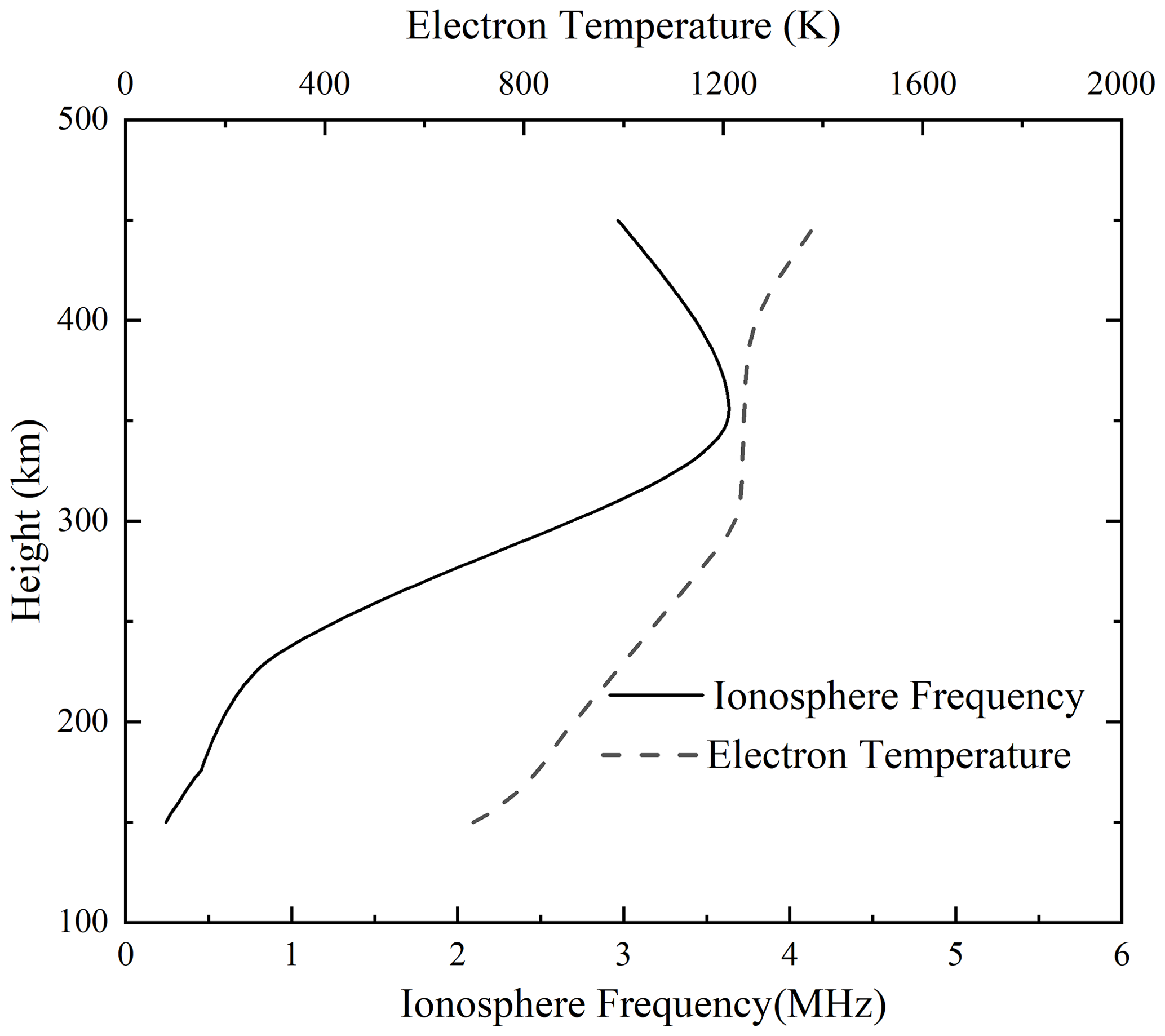
In this section, we analyze the drift current caused by ohmic heating according to the theoretical model developed in the preceding section. Background data are from the HAARP on 2 October 2011. The ionospheric and atmospheric background profiles are given by the International Reference Ionosphere (IRI) model (Bilitza et al., 2017) and the neutral atmosphere model (Mass Spectrometer Incoherent Scatter – MSIS) (Picone et al., 2002) as well as geomagnetic field data from the International Geomagnetic Reference Field (IGRF) model (Finlay et al., 2010). Figure 1 shows the background data. The critical frequency of the ionosphere is 3.67 MHz, and its altitude is 350 km.

The computational domain is −150 to 300 km in the x-axis direction and 150 to 450 km in the z-axis direction. The spatial grid size is 2 km. The effective radiated power (ERP) of the transmitter is set at 500 MW; the transmitting frequency is set at 4 MHz, which is greater than the ionospheric critical frequency. The transmitting half-width of the transmitter is set at 7^∘, and the transmitting waveform is an X wave.

Figure 1 Background ionospheric electron frequency and electron temperature.

3.1 Ionospheric heating effect and drift current

Based on the presented theory and parameters, we calculate the ionospheric heating results at θ=0. Figure 2 shows the change in the ionosphere after the heating is stable. Figure 2a shows that the maximum temperature change is ΔT_e ∼ 570 K when heating is stable, and the change ratio is $\mathrm{\Delta }{T}_{\mathrm{e}}/T_{\mathrm{e}}\sim \mathrm{48}$ %. The corresponding electron pressure is given in Fig. 2b; it is about $\mathrm{4.1}\times {\mathrm{10}}^{-\mathrm{9}}$ Pa in the center of the heated area. According to the pressure changes obtained from Fig. 2b, the ionosphere's current density distribution can be obtained by Eqs. (15) and (16). The results are shown in Fig. 2c and d, the maximum value of J_y is approximately $\mathrm{7.8}\times {\mathrm{10}}^{-\mathrm{10}}$ A m⁻², and J_x is approximately $\mathrm{9.3}\times {\mathrm{10}}^{-\mathrm{43}}$ A m⁻². The J_y direction is perpendicular to the magnetic field, and J_x is along the pressure gradient.

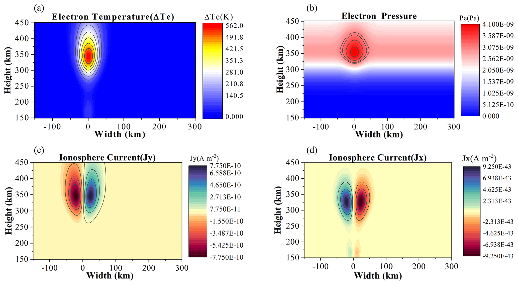
Figure 2 Ionospheric parameter when the heating is stable. (a) Electron temperature. (b) Electron pressure. (c) J_y current distribution. (d) J_x current distribution.

To characterize the impact of collisions on the current, we calculate various collision frequencies at the position of the ionospheric critical frequency and find v_en=2 Hz, v_in=0.29 Hz, and ω_ce=1.28 MHz. Therefore, ignoring the collision frequency of electrons and ions with neutral particles in Eqs. (13) and (14) is reasonable, and the equations can be solved to give

$$\begin{array}{}\text{(18)}& J_x\approx \mathrm{0},J_y\approx -e{\mathrm{\nabla }}_{\perp }{P}_{\mathrm{e}}/m{\mathit{\omega }}_{\mathrm{ce}}.\end{array}$$

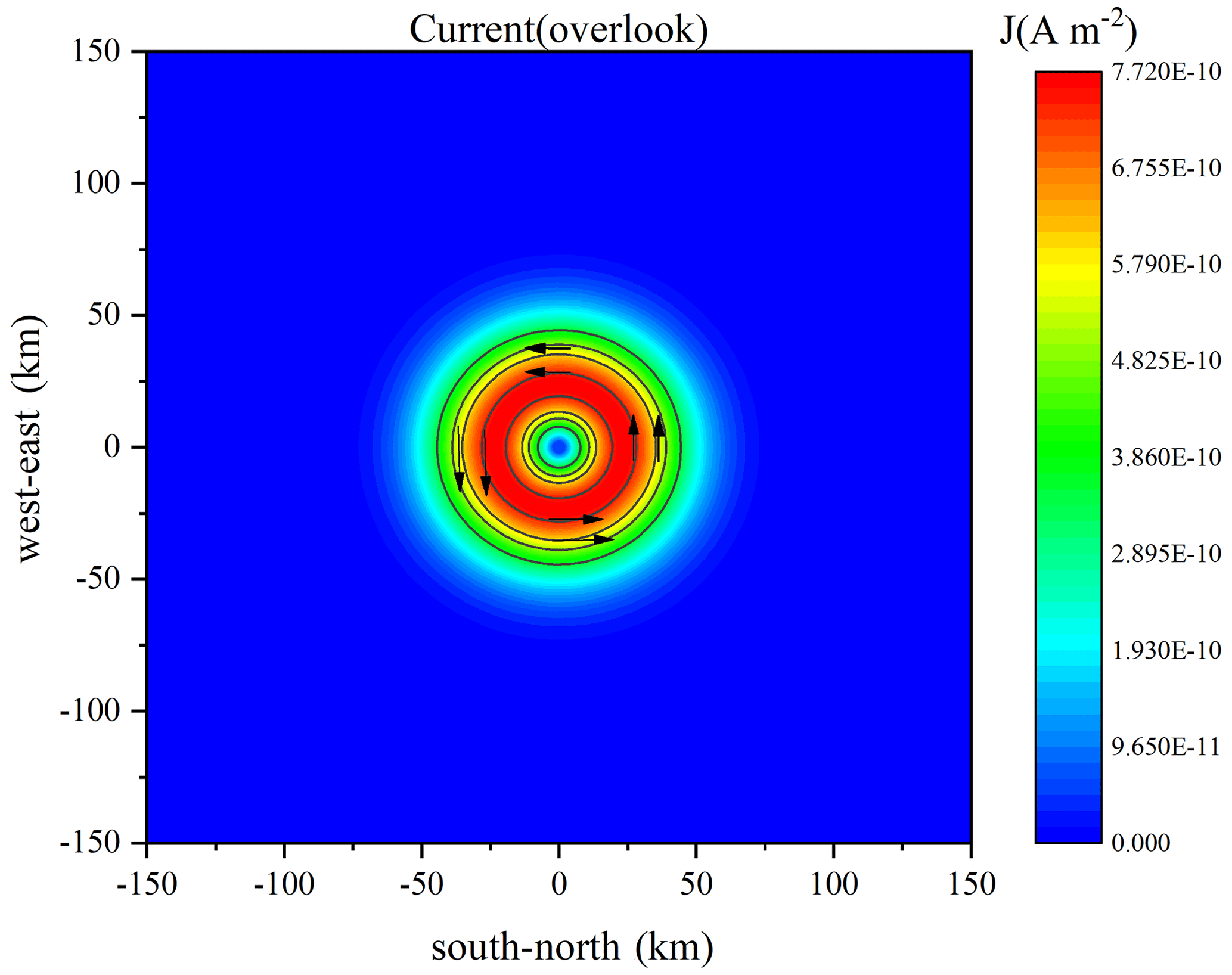
We can find that no current is generated in the x direction, and the current generated in the y direction is mainly a diamagnetic drift current. What is interesting about this simplification is that we do not constrain the electron–ion collisions, so the electron–ion collisions do not affect the F-layer drift current. When J_y is positive, the current flows inward perpendicular to the xz plane; when it is negative, the current flows outward. Therefore, the diamagnetic current is cylindrically symmetric about the z axis. The distribution of the current in the horizontal plane at the critical frequency position is shown in Fig. 3 (obtained by sweeping). The arrow in the figure indicates that the direction of the current flow is counterclockwise in this framework, with zero current in the heating center, gradually increasing and then decreasing towards the outside.

Figure 3 Horizontal distribution of the drift current at the critical frequency position.

3.2 Influence of different angles on the drift current

According to the Kotik et al. (2013) experimental results, the strongest low-frequency electromagnetic signal is received on the ground when the HF wave heating direction is parallel to the magnetic field, i.e., the direction of the magnetic zenith. The radiated signal decreases as the angle between the radio wave and the geomagnetic field increases. This section provides a theoretical explanation for this observation. We study the effects of different heating directions on the drift current by fixing other transmitter parameters and setting the angle θ = 10, 20, and 30^∘. The temperature change ΔT_e and the current J_y in the ionosphere are shown in Fig. 4. Figure 4a, c, and e show diagrams of electron temperature ΔT_e at θ = 10, 20, and 30^∘, respectively. It is obvious that, with an increase in θ, the heating area shifts horizontally and the heating effect gradually weakens. Figure 4b, d, and f show diagrams of current at θ = 10, 20, and 30^∘. The currents undergo the same kind of change as the temperature. The current is generally symmetric about the launching center axis.

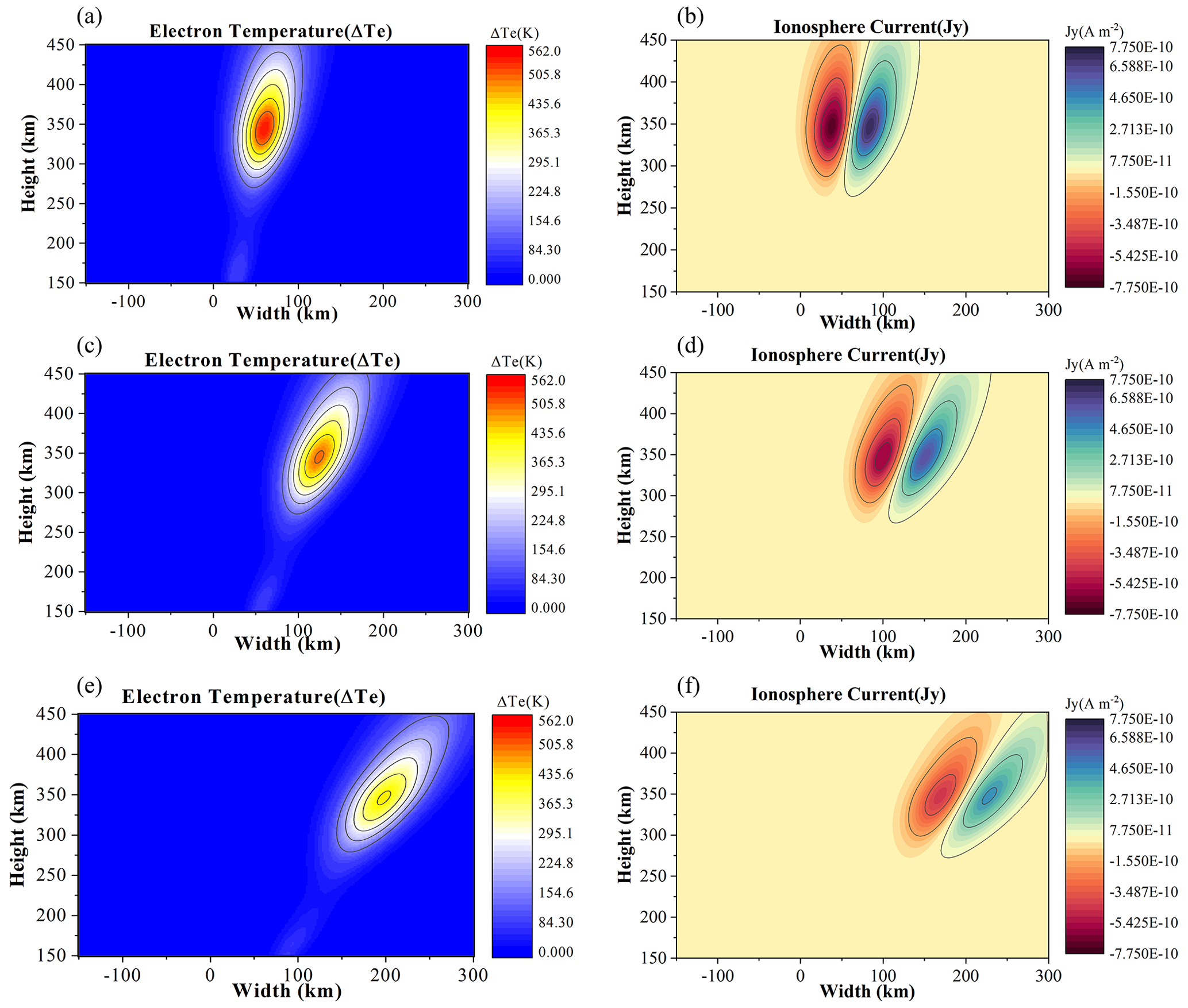
Figure 4 Distributions of (a) electron temperature at θ = 10^∘, (b) current J_y at θ=10^∘, (c) electron temperature at θ=20^∘, (d) current J_y at θ=20^∘, (e) electron temperature at θ=30^∘, and (f) current J_y at θ=30^∘.

In order to investigate the effects of angle θ more visually, we calculate the maximum temperature change for a different angle θ; this is shown by the red dots in Fig. 5. The electron temperature change is 560 K at θ=0 and is reduced to 430 K at θ=30^∘. We also performed a plane integration of the absolute values of the current density (avoiding positive and negative cancellation). The results are marked by the green triangles in Fig. 5. It can be seen that the current reaches 5.76 A during vertical heating and decreases gradually with increasing angles.

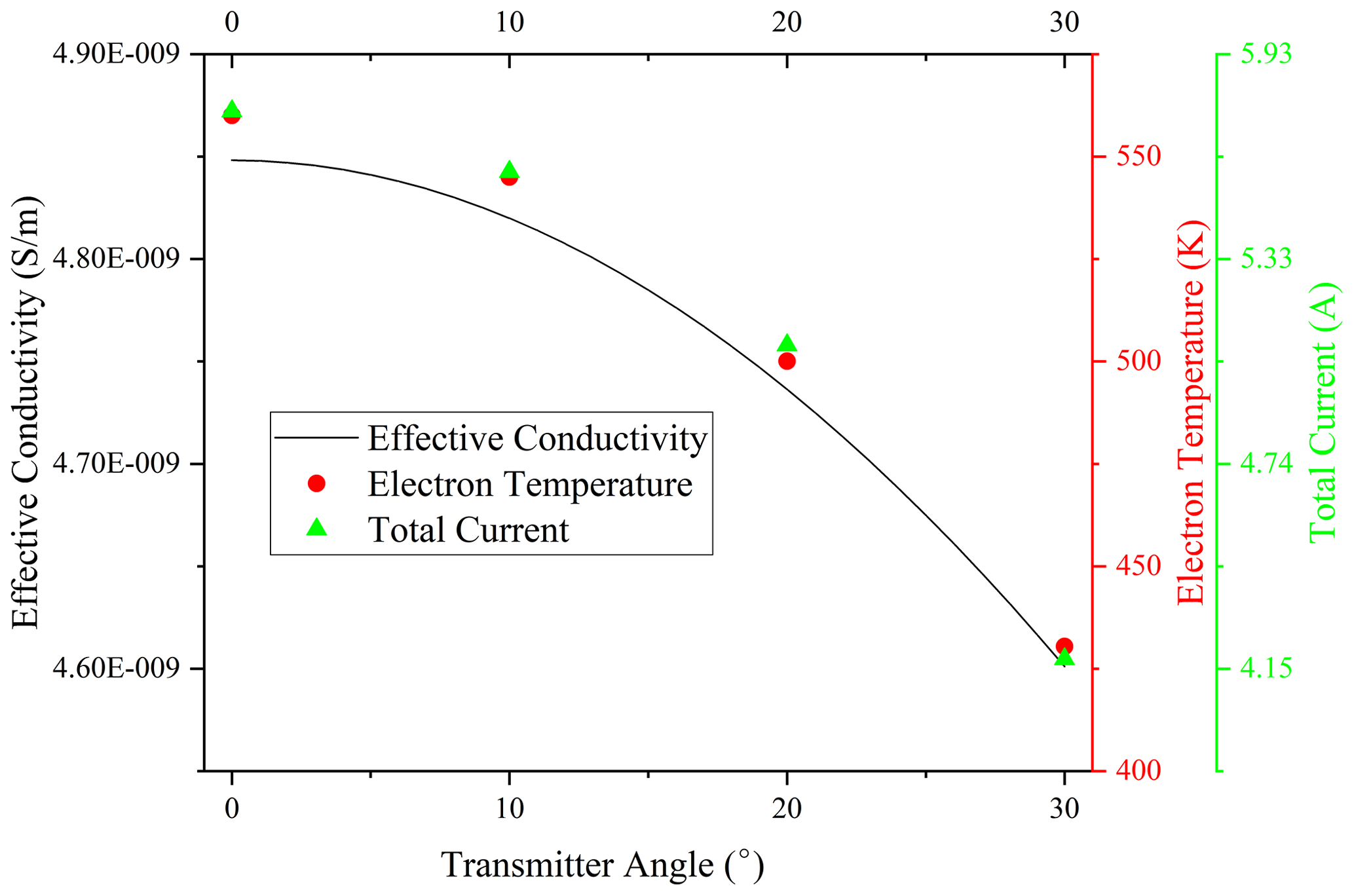
Figure 5 Effective conductivity, electron temperature, and total current as functions of angle θ.

To explore what causes the changes in electron temperature and current, we calculate the effective conductivity at different angles. Combining Eqs. (4) and (6), the dependence of effective conductivity on the angle can be derived.

$$\begin{array}{}\text{(19)}& \begin{array}{rl}{\mathit{\sigma }}_{\mathrm{ef}}& ={\displaystyle \frac{{\mathit{\epsilon }}_{\mathrm{0}}{\mathit{\omega }}_{\mathrm{pe}}^{\mathrm{2}}{v}_{\mathrm{e}}}{{\mathit{\omega }}^{\mathrm{2}}+v_{\mathrm{e}}^{\mathrm{2}}}}{\sin }^{\mathrm{2}}\left(\mathit{\theta }\right)+{\displaystyle \frac{{\mathit{\epsilon }}_{\mathrm{0}}{\mathit{\omega }}_{\mathrm{pe}}^{\mathrm{2}}{v}_{\mathrm{e}}}{\mathrm{2}}}\left(\right({\displaystyle \frac{\mathrm{1}}{(\mathit{\omega }-{\mathit{\omega }}_{\mathrm{ce}}{)}^{\mathrm{2}}+v_{\mathrm{e}}^{\mathrm{2}}}}\\ & +{\displaystyle \frac{\mathrm{1}}{(\mathit{\omega }+{\mathit{\omega }}_{\mathrm{ce}}{)}^{\mathrm{2}}+v_{\mathrm{e}}^{\mathrm{2}}}}\left)\right(\mathrm{1}+{\cos }^{\mathrm{2}}\left(\mathit{\theta }\right))\\ & +({\displaystyle \frac{\mathrm{1}}{(\mathit{\omega }-{\mathit{\omega }}_{\mathrm{ce}}{)}^{\mathrm{2}}+v_{\mathrm{e}}^{\mathrm{2}}}}-{\displaystyle \frac{\mathrm{1}}{(\mathit{\omega }+{\mathit{\omega }}_{\mathrm{ce}}{)}^{\mathrm{2}}+v_{\mathrm{e}}^{\mathrm{2}}}})\cos \left(\mathit{\theta }\right))\end{array}\end{array}$$

Choosing the ionospheric frequency, electron cyclotron frequency, collision frequency, and transmitter frequency at the corresponding heights, we obtain a relationship between the angle and the effective conductivity as shown by the black line in Fig. 5. It can be seen from the graph that the effective conductivity decreases gradually as the angle θ increases. We find that the trend of effective conductivity is the same as the trends of temperature and current. Physically, it is the change in effective conductivity that causes the change in heating. The conductivity is maximal when θ=0, where the heating effect is best and the current is greatest. The conclusion could provide a natural explanation for the signal reaching its maximum values when the beam is directed along the Earth's magnetic field in the Kotik et al. (2013) experiment.

3.3 Magnetic field variations in the heating area

Unlike the methodology employed by Papadopoulos et al. (2011a) to measure the ground magnetic signals excited by antimagnetic currents, we present computed results of magnetic signals in the heating ionospheric region, building upon the work of Lühr et al. (2004) and Manoj et al. (2006), who utilized satellites to investigate the equatorial electrojet. In MHD theory, the momentum equation is

$$\begin{array}{}\text{(20)}& \mathit{\rho }{\displaystyle \frac{\mathrm{d}\mathit{u}}{\mathrm{d}t}}=-\mathrm{\nabla }P+\mathit{j}\times \mathit{B},\end{array}$$

where ρ is the mass density, u is the fluid mass velocity, j is the electric current density, and p is the pressure. During heating, the pressure variation is mainly contributed by electrons, so we ignore the ionic pressure and only consider the electron pressure. In this paper, we mainly consider the steady state. Inserting Maxwell's equation $\mathrm{\nabla }\times \mathit{B}={\mathit{\mu }}_{\mathrm{0}}\mathit{j}$, we get

$$\begin{array}{}\text{(21)}& \mathrm{\nabla }\left(P_{\mathrm{e}}+{\displaystyle \frac{B^{\mathrm{2}}}{\mathrm{2}{\mathit{\mu }}_{\mathrm{0}}}}\right)={\displaystyle \frac{\mathrm{1}}{{\mathit{\mu }}_{\mathrm{0}}}}\left(\mathit{B}\cdot \mathrm{\nabla }\right)\mathit{B}.\end{array}$$

The right-hand side represents the magnetic tension due to the curvature of the field lines; it is negligible since the scale of the heated region is very small compared to the scale of the geomagnetic field (Alken et al., 2017). Thus, electron pressure will immediately be balanced by a decrease in magnetic pressure:

$$\begin{array}{}\text{(22)}& \mathit{\delta }{P}_{\mathrm{e}}+{\displaystyle \frac{B_{\mathrm{1}}^{\mathrm{2}}}{\mathrm{2}{\mathit{\mu }}_{\mathrm{0}}}}={\displaystyle \frac{B_{\mathrm{0}}^{\mathrm{2}}}{\mathrm{2}{\mathit{\mu }}_{\mathrm{0}}}},\end{array}$$

where B₀ is the undisturbed geomagnetic field, B₁ is the disturbed geomagnetic field, and δP_e is the variation of the electron pressure due to heating. Thus the change in the magnetic signal $\mathit{\delta }B=B_{\mathrm{0}}-B_{\mathrm{1}}$ induced by heating the ionosphere can be expressed as

$$\begin{array}{}\text{(23)}& \mathit{\delta }B=B_{\mathrm{0}}-\sqrt{B_{\mathrm{0}}^{\mathrm{2}}-\mathrm{2}{\mathit{\mu }}_{\mathrm{0}}{P}_{\mathrm{e}}}.\end{array}$$

Combined with the variation in electron pressure at θ = 0, 10, 20, and 30^∘, we can get the corresponding magnetic field variation δB in the heating region; the result is shown in Fig. 6. As shown in Fig. 6, it is clear that the magnetic field δB gradually decreases as the angle θ increases, which varies in the same way as the equivalent conductivity varies with the angle. When θ = 0, 10, 20, and 30^∘, the maximum values of the magnetic field are δB = 48, 47, 43, and 37 pT. Comparing the experimental results of Papadopoulos et al. (2011a; the maximum at the Earth's surface is only about 1 pT), one can find that the magnetic field in the heating region is much stronger than the strength of the magnetic field received at the ground surface, which indicates that the signal attenuates severely during the propagation process.

In this subsection, we calculated the magnetic field variation in the heating region based on the MHD theory. It is important to note that this calculation is only suitable for the heating region. A detailed calculation by propagation theory is needed to receive signals at a distance (ground). This paper's model is based on the background conditions at high latitudes. Extending to the middle and low latitudes requires a similar transformation of the conductivity tensor. Hence, this model is not applicable to the middle and low latitudes.

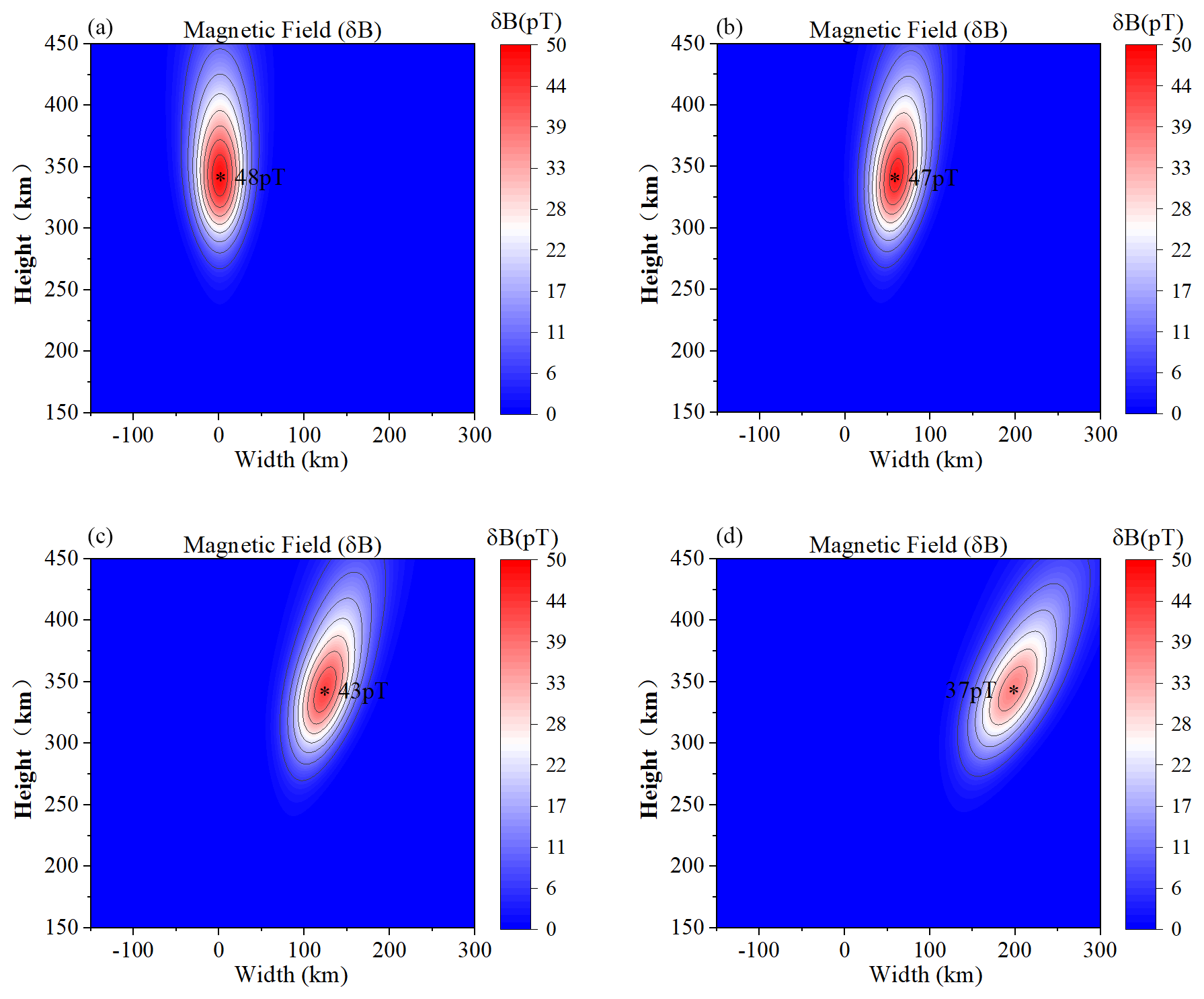
Figure 6 Distributions of (a) the magnetic field at θ=0, (b) the magnetic field at θ=10^∘, (c) the magnetic field at θ=20^∘, and (d) the magnetic field at θ=30^∘.

4 Conclusions

We establish a model of drift current in the ionosphere using the ohmic heating model and the MHD momentum equation and give the formulas to calculate the drift current and magnetic field variations in the heating area. The following conclusions are reached based on these calculations.

When the ERP is 500 MW and θ = 0^∘, the ionospheric electron temperature change ΔT_e is about 570 K, and the change ratio is $\mathrm{\Delta }{T}_{\mathrm{e}}/T_{\mathrm{e}}\sim \mathrm{48}$ %. From the calculated distribution of the drift current in the ionosphere, the maximum value of J_y is approximately $\mathrm{7.8}\times {\mathrm{10}}^{-\mathrm{10}}$ A m⁻², and J_x is approximately $\mathrm{9.3}\times {\mathrm{10}}^{-\mathrm{43}}$ A m⁻². The total current excited by heating is 5.76 A.

It is concluded that the collisions of charged particles with neutral particles have a negligible effect on the current; electron–ion collisions do not affect the drift current. The current is mainly a diamagnetic current and is ring-shaped, with zero at the center and gradually increasing outward until it decreases again.

An analytical equation of the dependence of the effective conductivity σ_ef on the emission angle θ is given. The effect of the emission angle θ on the electron temperature and current density is explained by using the concept of effective conductivity. The most substantial current is obtained when the X wave heats the ionosphere along the magnetic field direction, and the current gradually decreases as the angle θ increases. Theoretically, this explains why the strongest signal is received by the ground when heated along the magnetic inclination angle.

We give an equation for the magnetic field variation in the heating region. The calculation results show that the emission angle is θ = 0, 10, 20, and 30^∘ and that the maximum value of the magnetic field is δB = 48, 47, 43, and 37 pT. The position of the maximum variation of the magnetic field is at the center of the heating area.