The altitude of green OI 557.7 nm and blue N₂⁺ 427.8 nm aurora

We have performed a large statistical study of the peak emission altitude of green O(¹D₂–¹S₀) (557.7 nm) and blue ${\mathrm{N}}_{\mathrm{2}}^{+}$ 1 N (427.8 nm) aurora using observations from a network of all-sky cameras stationed across northern Finland and Sweden recorded during seven winter seasons from 2000 to 2007. Both emissions were found to typically peak at about 114 km. The distribution of blue peak altitudes is more skewed than that for the green, and the mean peak emission altitudes were 114.84 ± 0.06 and 116.55 ± 0.07 km for green and blue emissions, respectively. We compare simultaneous measurements of the two emissions in combination with auroral modelling to investigate the emission production mechanisms.

During low-energy electron precipitation ($<\sim$ 4 keV), when the two emissions peak above about 110 km, it is more likely for the green emission to peak below the blue emission than vice versa, with the difference between the two heights increasing with their average. Modelling has shown that under these conditions the dominant source of O(¹S), the upper state of the green line, is energy transfer from excited N₂ ($A^{\mathrm{3}}{\mathrm{\Sigma }}_{\mathrm{u}}^{+}$), with a rate that depends on the product of the N₂ and O number densities. Since both number densities decrease with higher altitude, the production of O(¹S) by energy transfer from N₂ peaks at lower altitude than the N₂ ionisation rate, which depends on the N₂ number density only. Consequently, the green aurora peaks below the blue aurora.

When the two emissions peak below about 110 km, they typically peak at very similar altitude. The dominant source of O(¹S) at low altitudes must not be energy transfer from N₂, since the rate of that process peaks above the N₂ ionisation rate and blue emission due to quenching of the long-lived excited N₂ at low altitudes. Dissociative recombination of ${\mathrm{O}}_{\mathrm{2}}^{+}$ seems most likely to be a major source at these low altitudes, but our model is unable to reproduce observations fully, suggesting there may be additional sources of O(¹S) unaccounted for.

1 Introduction

The emission height of the aurora is often used in the derivation of other auroral or ionospheric parameters, such as horizontal spatial scales, velocities, or electron precipitation energies (e.g. Kaila, 1989; Knudsen et al., 2001; Kalmoni et al., 2017), or as a height of other measurements such as neutral wind and temperature (e.g. Griffin et al., 2006; Kosch et al., 2011; Billett et al., 2020). Usually an assumption must be made about the height of the aurora. These assumptions are typically based on observations conducted using instruments and techniques which are primitive by modern standards (Störmer, 1916; Harang, 1951; Störmer, 1955). Often, earlier work measured the “lower border” of an auroral arc, which is dependent on the instrument sensitivity (as pointed out by Boyd et al., 1971 and Whiter et al., 2013), and therefore results using such methods should be treated with caution. The present study was motivated by the need to improve estimates of the auroral peak emission height and utilises tens of thousands of camera images for which a single peak emission height has been derived for each pair of coincident auroral images, enabling a large statistical study. In this work we analyse two of the brightest (and most observed) auroral emissions: the OI 557.7 nm “green line” and the ${\mathrm{N}}_{\mathrm{2}}^{+}$ 427.8 nm “blue line”.

The auroral green line is an atomic oxygen emission, from the O(¹D₂–¹S₀) transition, while the blue line is a feature of the ${\mathrm{N}}_{\mathrm{2}}^{+}$ First Negative (1 N) band system (${\mathrm{B}}^{\mathrm{2}}{\mathrm{\Sigma }}_{\mathrm{u}}^{+}$–${\mathrm{X}}^{\mathrm{2}}{\mathrm{\Sigma }}_{\mathrm{g}}^{+}$). However, despite coming from species with different number density altitude profiles, it has been known for some decades that the green and blue auroral emissions have more similar height profiles than their parent species would suggest (Henriksen and Egeland, 1988). This similarity is thought to be because the usual primary route by which O(¹S) is produced in aurora is energy transfer from electronically excited N₂ in the $A^{\mathrm{3}}{\mathrm{\Sigma }}_{\mathrm{u}}^{+}$ state (Henriksen, 1973; Sharp and Torr, 1979; Burns and Reid, 1984; Gerdjikova and Shepherd, 1987; Gattinger et al., 1996) (we hereafter abbreviate to N₂(A)). However, there are several other pathways producing O(¹S) in the aurora, including dissociative recombination of ${\mathrm{O}}_{\mathrm{2}}^{+}$, electron impact excitation of atomic O, and electron impact dissociation of O₂, and the balance of these (and other) pathways under different electron precipitation conditions is not yet well understood. In a companion study to this one, Partamies et al. (2022) investigate variation in the peak emission height of green OI 557.7 nm aurora with magnetic local time (MLT) and solar wind driving, over both Lapland (nightside auroral oval) and Svalbard (dayside cusp, nightside poleward edge of oval). Here we present average peak heights for both emissions over Lapland, before examining the difference in height between coincident green and blue auroral emission in combination with modelling to investigate the emission production mechanisms. We examine statistics compiled from individual time instants treated as independent measurements; the temporal evolution of auroral heights, for example, over the course of specific events, will be considered in a separate study.

Section 2 describes the imaging instrumentation used in this work and briefly summarises the method of determining auroral peak emission heights developed by Whiter et al. (2013). Observational results are presented in Sect. 3. Section 4 explains how the green and blue line emissions are modelled, and a detailed comparison of model results with observations is presented in Sect. 5.

Table 1 Locations (geographic latitude and longitude) of the camera stations used in this work.

2 Instrumentation and image analysis

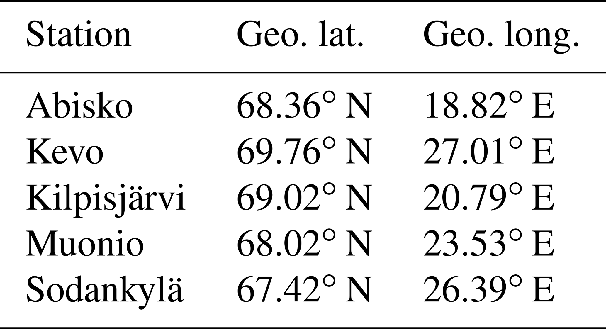
This work uses images from five ground-based all-sky cameras stationed across northern Finland and Sweden, which form part of the Magnetometers–Ionospheric Radar–All-sky Cameras Large Experiment (MIRACLE) instrument network (Syrjäsuo et al., 1998). The geographic locations of the stations used in this work are listed in Table 1. The fields of view of all of the cameras overlap, allowing for determination of the auroral peak emission height using any pair of stations. The cameras operate automatically throughout the winter, producing many tens of thousands of images per station per year. From 1996 to 2007, MIRACLE primarily used charge-coupled device (CCD) detectors equipped with an image intensifier (ICCD cameras) and narrow-passband interference filters to select specific auroral emissions, mounted within a filter wheel. This work has used images of OI 557.7 nm emission (green), which is the most dominant auroral emission, and N${}_{\mathrm{2}}^{+}$ 1 N 427.8 nm emission (blue), recorded with the ICCD cameras. Green images are available for the full time period of ICCD observations, whereas blue images are only available from September 2000 onwards. Only images recorded when the solar zenith angle at the camera station was larger than 101^∘ and the IL index (a local analogue of the AL index computed from MIRACLE magnetometer data; Kauristie et al., 1996) was less than −50 nT are used in this study, to exclude conditions of sunrise and sunset and to ensure that there was auroral activity.

All MIRACLE ICCD camera images recorded between 2000 and 2007 (the period when at least two mainland stations were available and both green and blue emissions were measured) have been analysed using two fully automated independent methods for computing the auroral peak emission height. These methods have been described in detail by Whiter et al. (2013). Both methods analyse a pair of coincident images from different stations with overlapping fields of view. One of the methods (the “field line method”) involves projecting all-sky images onto many geomagnetic field lines, while the other method (the “horizontal plane method”) involves projecting the images onto planes parallel to the Earth's surface at different heights. Since the aurora is typically taller than it is wide, in general the field line method gives a more accurate measure of the peak emission height, and all height data shown in this work were obtained using the field line method with a precision of 0.5 km. However, to ensure measurements are reliable, only image pairs for which the two methods agree to within 20 km are included in the statistical analysis. Of these, there are 57 907 simultaneous measurements of the height of both green and blue emissions from the same station pair (since the cameras use filter wheels to select each individual emission, there is approximately 2 s between the beginning of the green exposure and the beginning of the following blue exposure, which is comparable to the exposure time and short enough to consider the images to be simultaneous). The uncertainty of each individual height measurement is difficult to determine and varies with type of aurora and geometrical properties of the aurora but is estimated to be ± 1–10 km. Importantly, Whiter et al. (2013) showed that the field line method is not biased towards high or low altitudes, so the uncertainty is not systematic. A degradation of the instruments' image intensifiers would lead to a decrease in the minimum observable radiance, but the methods used here to find the peak emission height do not depend on absolute intensity, and therefore it is possible to combine images from different instruments without significant bias.

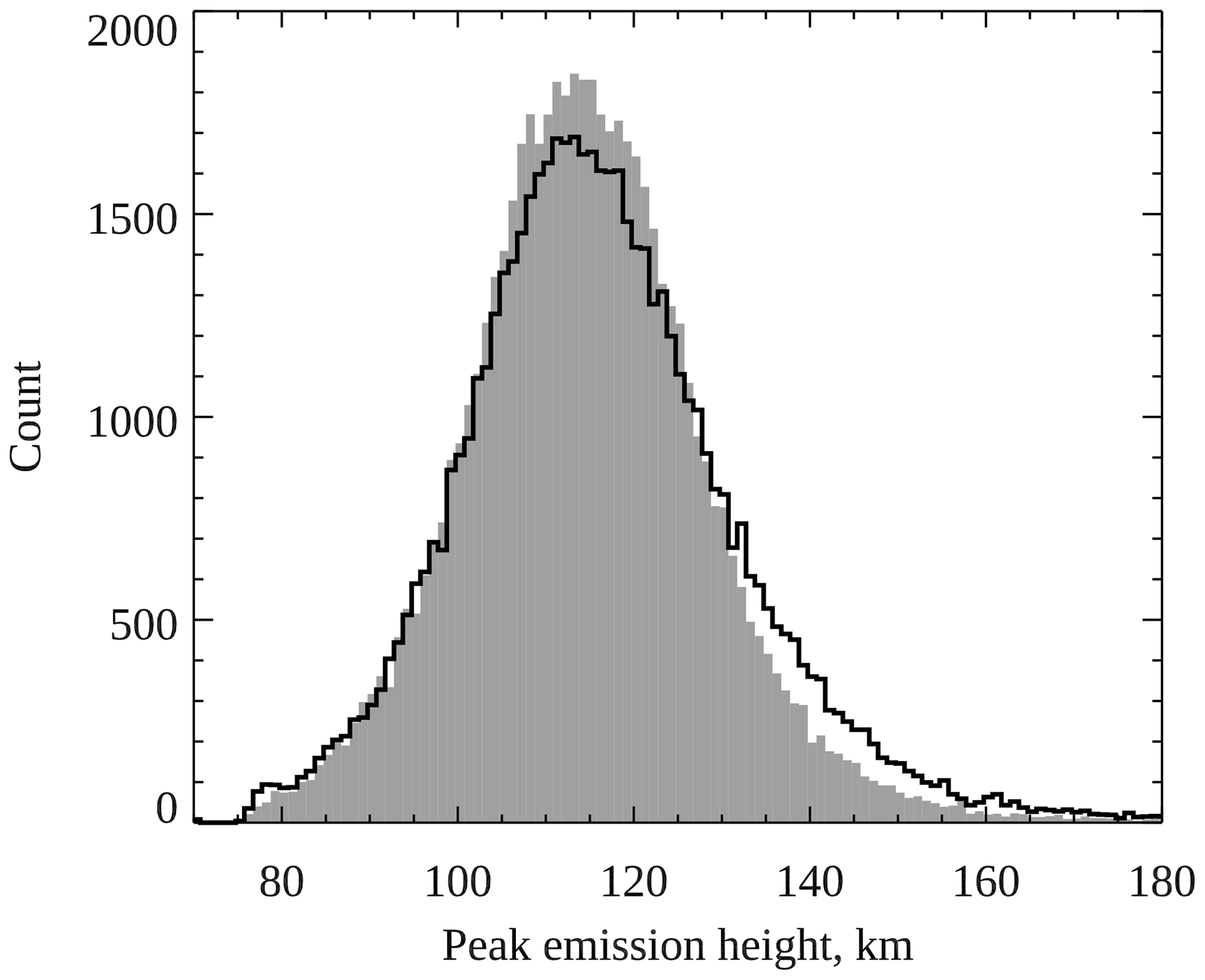
Figure 1 Histograms of observed peak emission heights for the green 557.7 nm emission (grey shading) and blue 427.8 nm emission (black outline).

Figure 2 The peaks of the histograms as shown in Fig. 1, together with Gaussian curves fitted to the histograms for the 557.7 nm emission (green) and 427.8 nm emission (blue). The vertical green and blue lines mark the peaks of the Gaussians.

3 Observational results

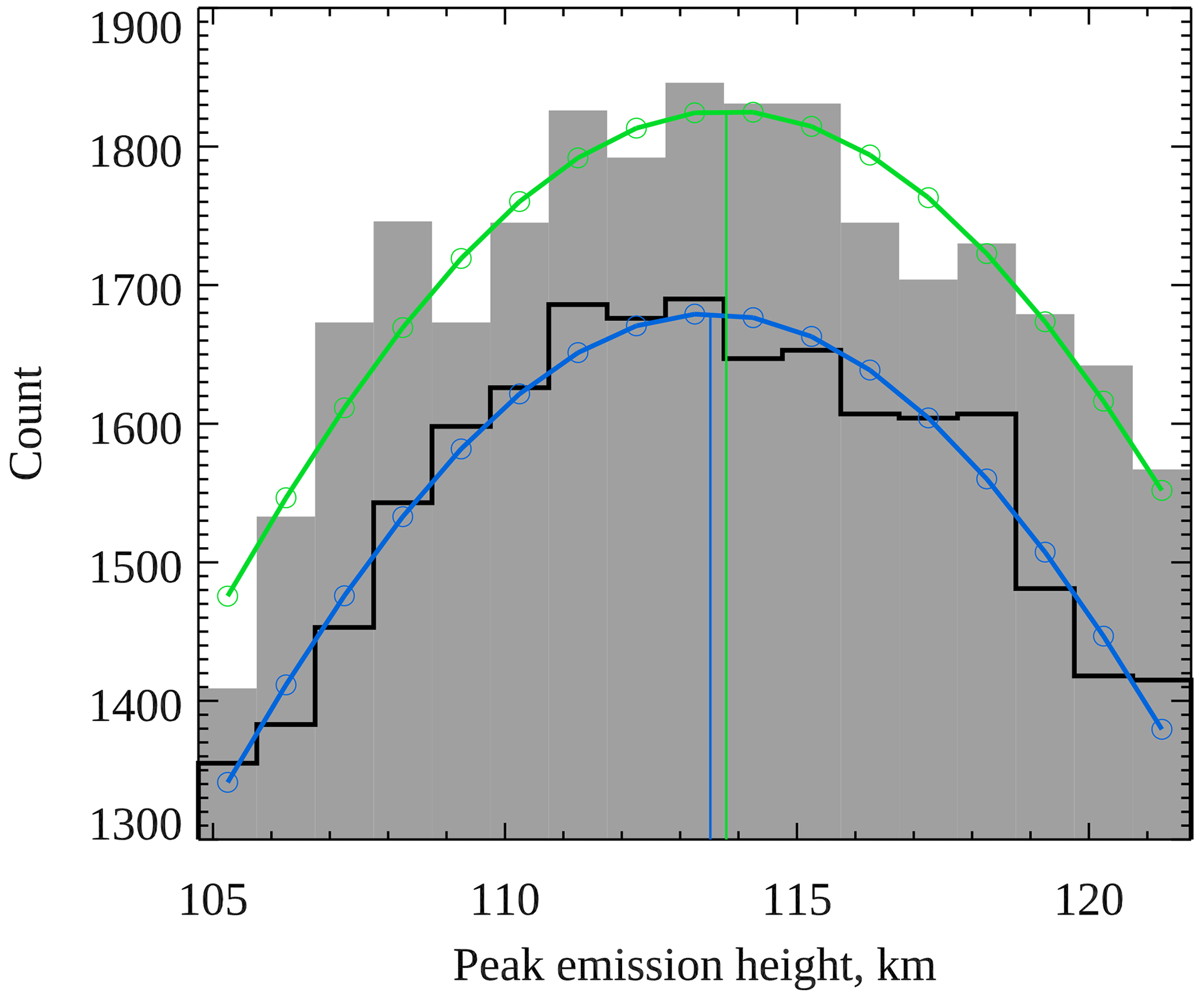
Figure 1 shows histograms of measured peak emission heights of green 557.7 nm aurora (shaded grey) and blue 427.8 nm aurora (black line), with a bin width of 1 km. Only measurements at times when height estimates of both emissions are available are included in the histograms, in order to allow for a fair comparison. Both distributions peak close to 114 km and have very similar tails towards lower peak emission heights. However, the distribution of green heights has a steeper tail towards greater peak emission heights than the distribution of blue heights. These histograms show that the blue line is almost twice as likely (factor 1.8) to peak at 140 km as the green line, although it is rare for either of these emissions to peak at such high altitudes. The median peak emission heights for green and blue aurora are 114.0 and 115.0 km respectively (to nearest 0.5 km), and the corresponding mean heights are 114.84 ± 0.06 km and 116.55 ± 0.07 km, suggesting that the blue line emission peaks slightly above the green line emission. In order to find the maxima of the distributions, a Gaussian function was fitted to each of the histograms plotted in Fig. 1 within the range 105.0–121.5 km (centred roughly on the peak of the distributions). Figure 2 shows the two histograms within this range, together with the fitted Gaussians in green (for 557.7 nm emission) and blue (for 427.8 nm emission). The coloured vertical lines within this figure show the maxima of the Gaussian functions, at 113.8 km for green aurora and 113.5 km for blue aurora. These results show that green and blue aurora peak at very similar altitudes, on average, but that it is more likely for blue to peak at high altitudes (above about 130 km) than green, contrary to a common misconception that blue peaks below green.

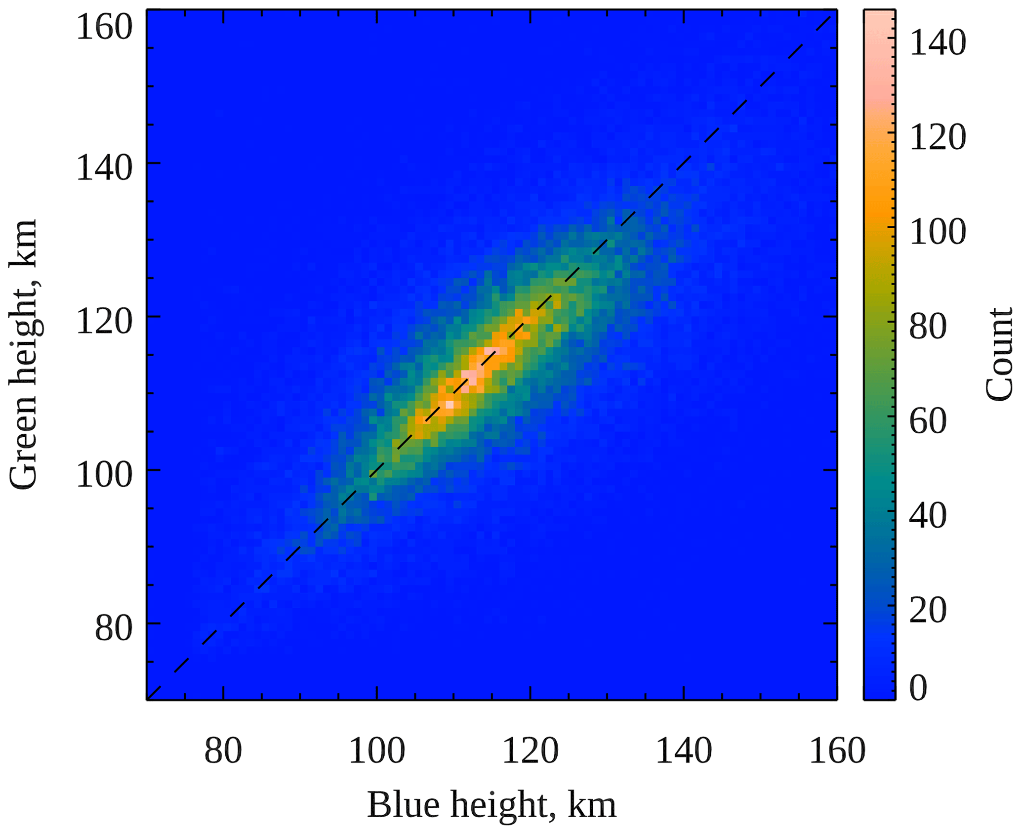
Figure 3 Two-dimensional histogram of simultaneous green (557.7 nm) and blue (427.8 nm) peak emission heights. The shading represents the number of observations in each histogram bin, according to the colour bar scale shown on the right of the figure. The dashed black line indicates where the two peak emission heights are equal.

In order to compare the peak emission heights of coincident green and blue aurora, a two-dimensional histogram was created, shown in Fig. 3. The bin width is 1 km for both green aurora (ordinate) and blue aurora (abscissa), and each 1 km × 1 km square is shaded according to the colour scale on the right of the figure to indicate the number of simultaneous height measurements of green and blue aurora within the ranges of that bin. The dashed diagonal line indicates where the two emissions peak at the same height (y=x line). The bulk of the distribution between 105 and 120 km closely follows this line, indicating that in general the two emissions peak at approximately the same altitude, as expected from the results presented above. At greater heights the majority of the distribution is below the dashed line, indicating that when the blue emission peaks at relatively high altitude, the green emission peaks below it.

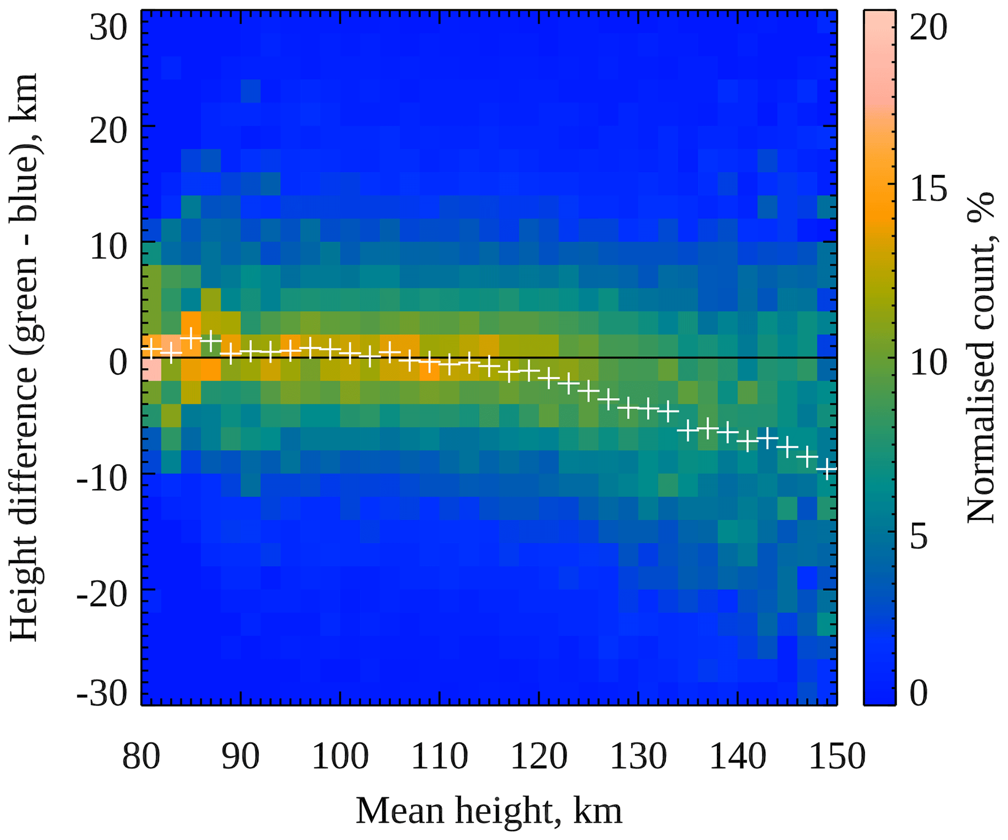
Figure 4 Two-dimensional histogram of auroral peak emission height observations binned according to the difference between green and blue heights (ordinate, positive values indicating green height above blue height) and mean (i.e. midpoint) of the simultaneous green and blue heights (abscissa). The shading represents the number of observations in each bin, normalised to the total number of observations in each column, according to the colour bar scale. The mean height difference for each column is shown as a white plus symbol.

This result can be seen more clearly by plotting the difference in height between the green and blue emissions against the mean height (i.e. midpoint between the green and blue heights). Figure 4 shows a two-dimensional histogram with the height difference (positive values indicating that the green emission peaks above the blue emission) on the ordinate axis and the mean height on the abscissa axis. The histogram bins have a width of 2 km in each direction, and the colour scale indicates the number of image pairs in each bin, normalised by the total number of image pairs in each column of the histogram. The white plus symbols show the mean height difference for each column of the histogram. As expected from the results shown in Fig. 3, the height difference is close to zero for mean heights up to about 120 km. As the mean height increases beyond 120 km, the average height difference becomes more negative, indicating that the blue emission peaks further above the green emission. The mean height was above 120 km in 34 % of our observations.

3.1 Resonance scattering of sunlight by N${}_{\mathrm{2}}^{+}$

In sunlit conditions, ${\mathrm{N}}_{\mathrm{2}}^{+}$ 1 N emission is produced through resonance absorption of solar photons by ${\mathrm{N}}_{\mathrm{2}}^{+}$ molecules in the ground state (Bates, 1949; Broadfoot, 1967). The resonance scattering contribution to the total blue line intensity can be significant and typically occurs at higher altitude than the auroral emission produced by electron impact excitation (Jokiaho et al., 2009). The auroral emission is prompt and produced at the point of ionisation and therefore is related to the altitude profile of the neutral N₂ density. Blue line emission originating through resonance scattering is instead related to the ${\mathrm{N}}_{\mathrm{2}}^{+}$ ion density and so is enhanced by soft electron precipitation producing ground-state ${\mathrm{N}}_{\mathrm{2}}^{+}$ above the shadow height and may also be influenced by ion transport.

To investigate whether the observed high peak altitude of the blue line could be caused by resonance scattering of sunlight, histograms were created for the solar zenith angle and MLT at the time of the observations. Data were selected where the blue line peaked above 130 km and at least 10 km above the coincident green line peak emission height, consisting of 8.7 % of the total height measurements. Histograms were made separately for this selected data and all other unselected data, shown in Fig. 5 (solar zenith angle) and Fig. 6 (MLT). The solar zenith angle and MLT were calculated for the central latitude and longitude of the aurora, defined to be on the field lines used in the calculation of the peak emission height, rather than for the observation stations, to improve accuracy.

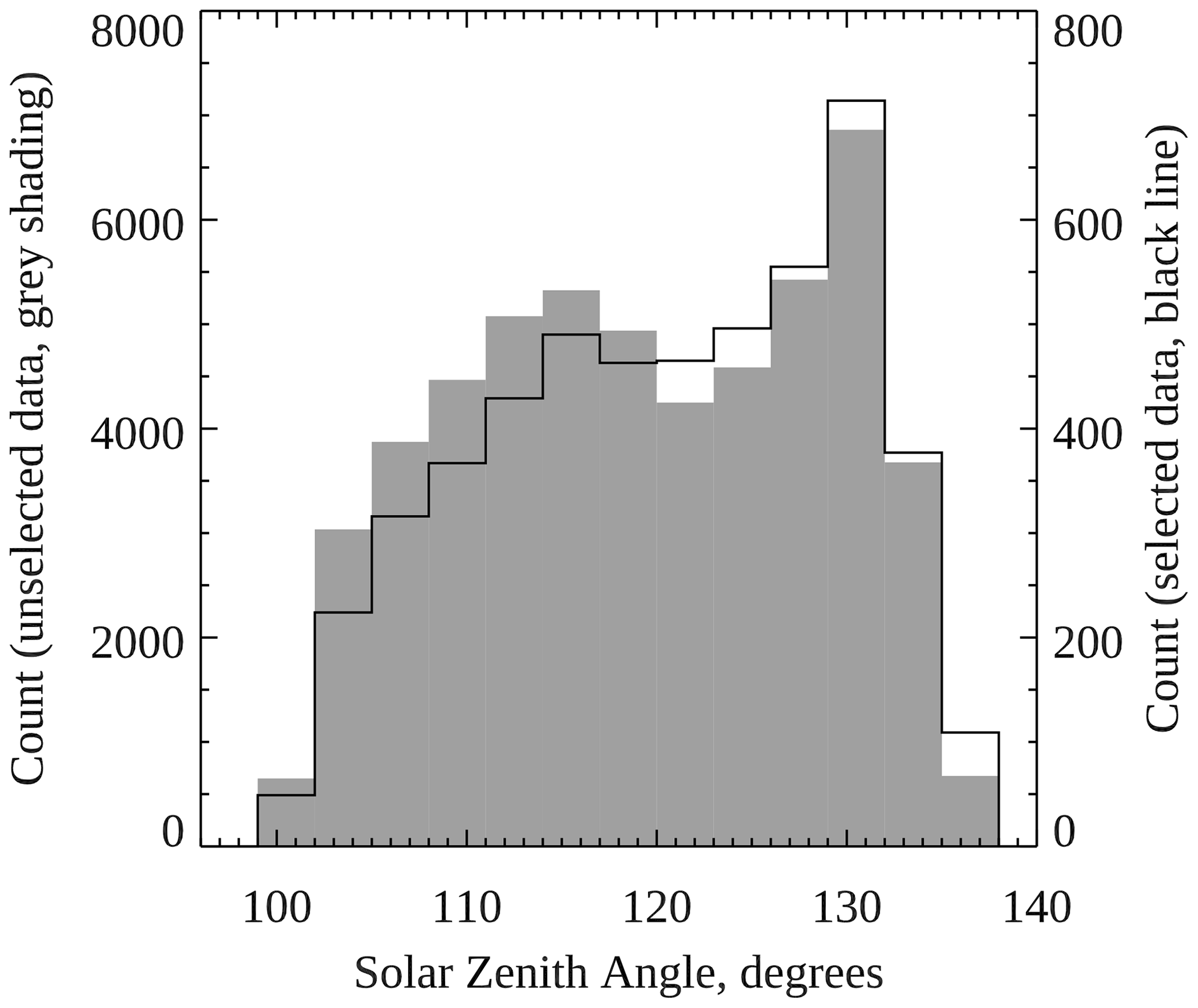
Figure 5 Histogram of the solar zenith angle at the time of the peak emission height measurements. The black line shows selected data (blue height above 130 km and at least 10 km above the green height) using the right ordinate axis, and the grey shading shows all remaining unselected data using the left ordinate axis.

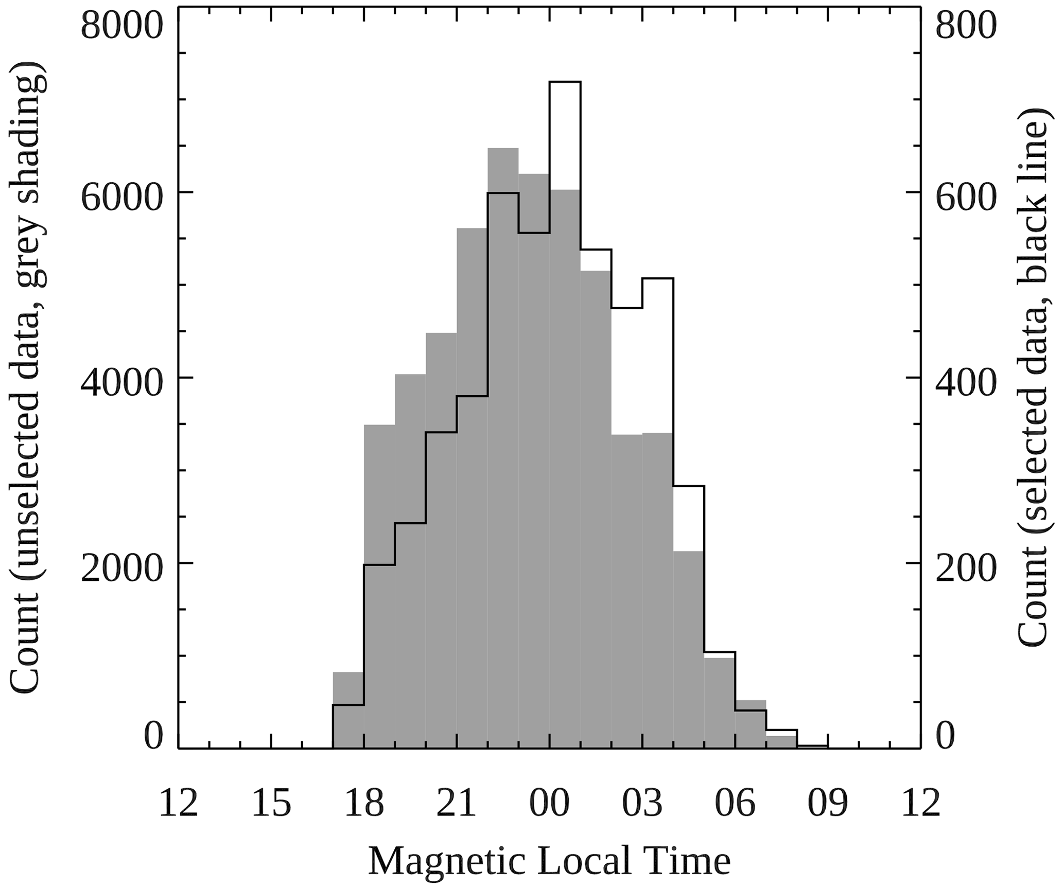
Figure 6 Histogram of the magnetic local time of the peak emission height measurements. The black line shows selected data (blue height above 130 km and at least 10 km above the green height) using the right ordinate axis, and the grey shading shows all remaining unselected data using the left ordinate axis.

These histograms show that the high blue peak emission heights do not preferentially occur for low solar zenith angles or close to dawn or dusk and therefore are not likely to be caused by resonance scattering of sunlight (or by daylight contamination on the horizon). The selected data are more centred around midnight MLT than the unselected data, but the two histograms shown in Fig. 6 are not substantially different. See the companion paper by Partamies et al. (2022) for further discussion of the variation in height with MLT.

4 Auroral modelling

We use the Southampton ionospheric model as a tool to understand the observational results presented in Sect. 3. This model is a coupled electron transport (Lummerzheim and Lilensten, 1994) and time-dependent ion chemistry model (Lanchester et al., 2001) which calculates production and loss rates for various ion and neutral species as well as brightnesses of specific auroral emissions (Lanchester and Gustavsson, 2012; Whiter et al., 2012). The inputs to the model are an arbitrary electron precipitation spectrum and density profiles for the major neutrals (O, N₂, and O₂) taken from the NRLMSIS 2.0 model (Emmert et al., 2021), hereafter referred to as MSIS. In this work we use Gaussian- or Maxwellian-shaped electron precipitation spectra, as has been standard in auroral physics (e.g. Strickland et al., 1993; Tanaka et al., 2006). As input to MSIS we use median conditions during the observations presented in Sect. 3, of Ap =17, F10.7 =129, 81 d average F10.7 =129, and a time of 21:30 UT at Kilpisjärvi (69.02^∘ N, 20.79^∘ E).

The brightness of the blue line is calculated directly from the production rate of ${\mathrm{N}}_{\mathrm{2}}^{+}$ through electron impact ionisation of neutral N₂. Since the emission is prompt, its brightness can be calculated directly from the ionisation–excitation rate. The lifetime of the ${\mathrm{N}}_{\mathrm{2}}^{+}$ 1 N(0,1) band is 270 ns, as obtained from the Einstein coefficient given by Gilmore et al. (1992) (note this is long compared to the lifetime of the overall ${\mathrm{N}}_{\mathrm{2}}^{+}$ 1 N band system but is appropriate for the 427.8 nm emission), which is too fast for quenching to have a significant effect on the peak emission height. Using quenching rate coefficients for the ${\mathrm{N}}_{\mathrm{2}}^{+}$ ${\mathrm{B}}^{\mathrm{2}}{\mathrm{\Sigma }}_{\mathrm{u}}^{+}$ state from Valk et al. (2010), together with N₂ and O₂ densities from the model and the quenching equation given by Vallance Jones and Gattinger (1978), we estimate less than 1 % of the blue emission is quenched at 90 km altitude.

Green and Stolarski (1972)LeClair and McConkey (1993)Sheehan and St.-Maurice (2004)Kella et al. (1997)Gattinger et al. (1985)Piper (1982)Gattinger et al. (1996)

Table 2 Reactions producing O(¹S) included in the Southampton ionospheric model.

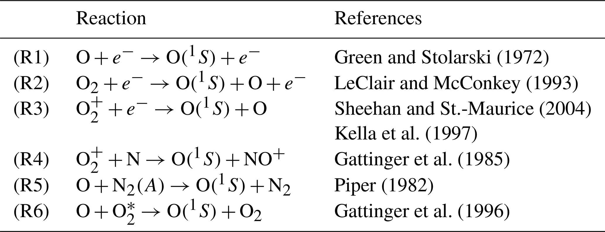
The 557.7 nm green line is long-lived, and therefore quenching is important, and so its intensity is calculated from the number density of the O(¹S) upper state with an Einstein coefficient of 1.26 s⁻¹ from Wiese et al. (1996). The reactions that produce O(¹S) included in the model are listed in Table 2, together with references for their cross sections, rate coefficients, and branching ratios, where relevant. Reactions (R1) and (R2) represent auroral electron impact on O and O₂, respectively. Reaction (R3) is dissociative recombination of ${\mathrm{O}}_{\mathrm{2}}^{+}$, and Reaction (R4) is an ${\mathrm{O}}_{\mathrm{2}}^{+}$ loss reaction with atomic N. Reactions (R5) and (R6) represent energy transfer to atomic O from N₂ and O₂, respectively. The model includes losses of O(¹S) through quenching by O and O₂ and losses through emission in 557.7 nm (lower state O(¹D)) and 297.2 nm (lower state O(³P)). Further discussion of the rates relevant for the green line emission is included in the following section.

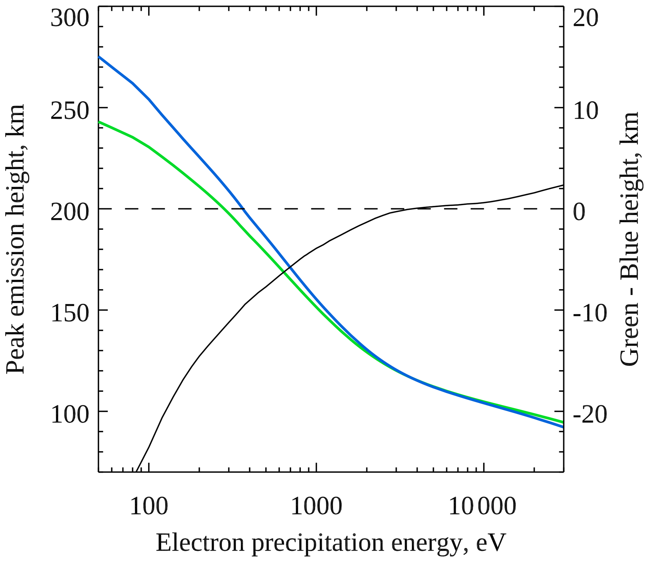
Figure 7 Peak emission heights of 557.7 nm aurora (green) and 427.8 nm aurora (blue) as a function of characteristic electron precipitation energy for Gaussian electron spectra, obtained using the Southampton ionospheric model. The difference in these heights is shown in black, using the right ordinate axis.

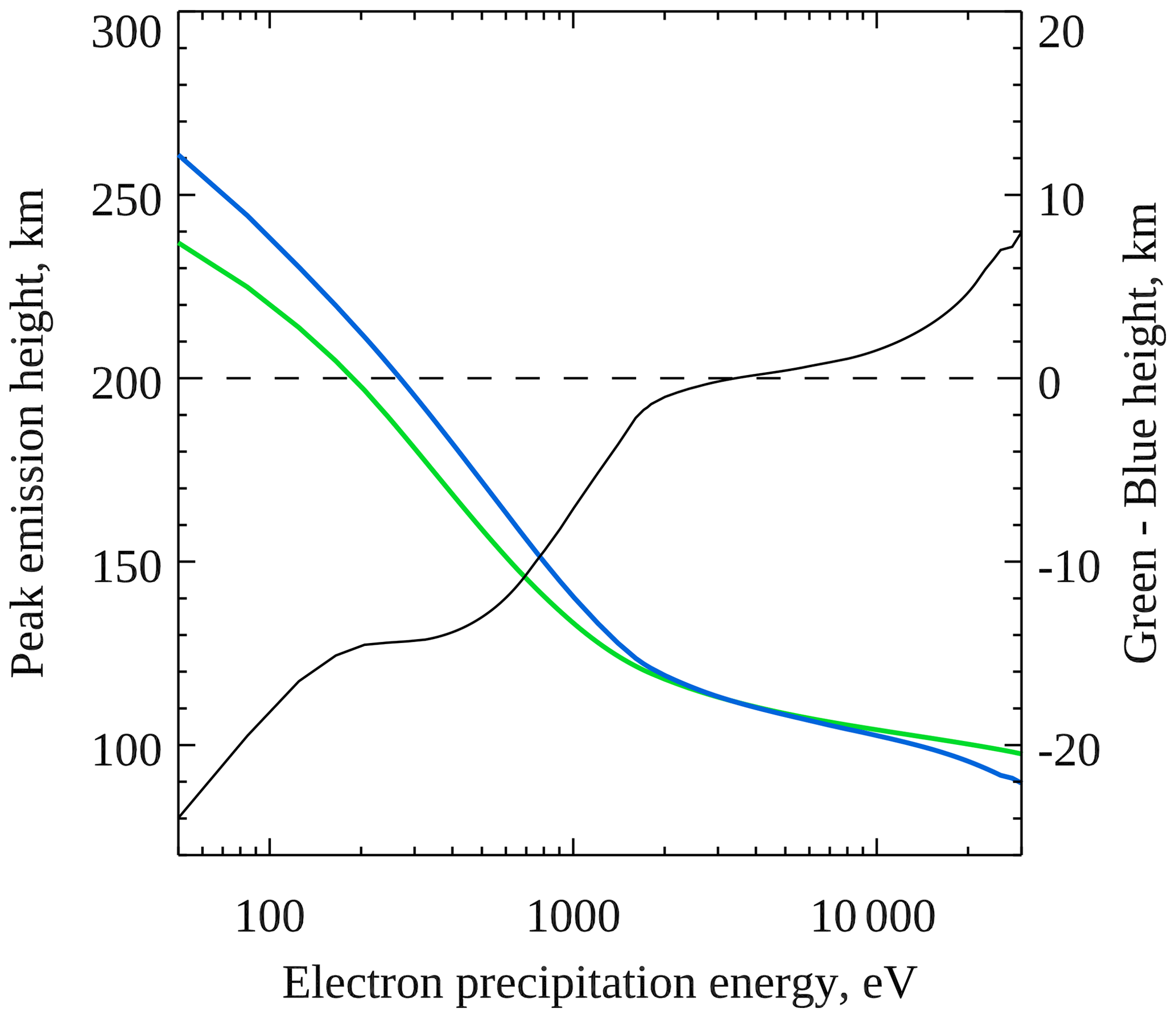
Figure 8 Peak emission heights of 557.7 nm aurora (green) and 427.8 nm aurora (blue) as a function of characteristic electron precipitation energy for Maxwellian electron spectra, obtained using the Southampton ionospheric model. The difference in these heights is shown in black, using the right ordinate axis.

5 Model results and comparison with observations

Figures 7 and 8 show the modelled peak emission heights of the 557.7 nm (green) and 427.8 nm (blue) lines as a function of characteristic electron precipitation energy with a Gaussian (Fig. 7) or Maxwellian (Fig. 8) electron spectrum. The difference in these heights (blue height subtracted from green height) is also shown in black, according to the right ordinate axis in each figure. To determine these relationships, the model was run independently at different characteristic energies with an electron energy flux of 20 mW m⁻² and at each energy was run for a period of 12 s in order to reach a reasonably steady state. Qualitatively, the model results resemble the observations presented in Sect. 3, in that the green and blue emissions peak at about the same height across much of the electron energy range tested, and at low energies, when the emissions peak at higher altitudes, the blue emission peaks above the green emission (more negative values on the right ordinate axis).

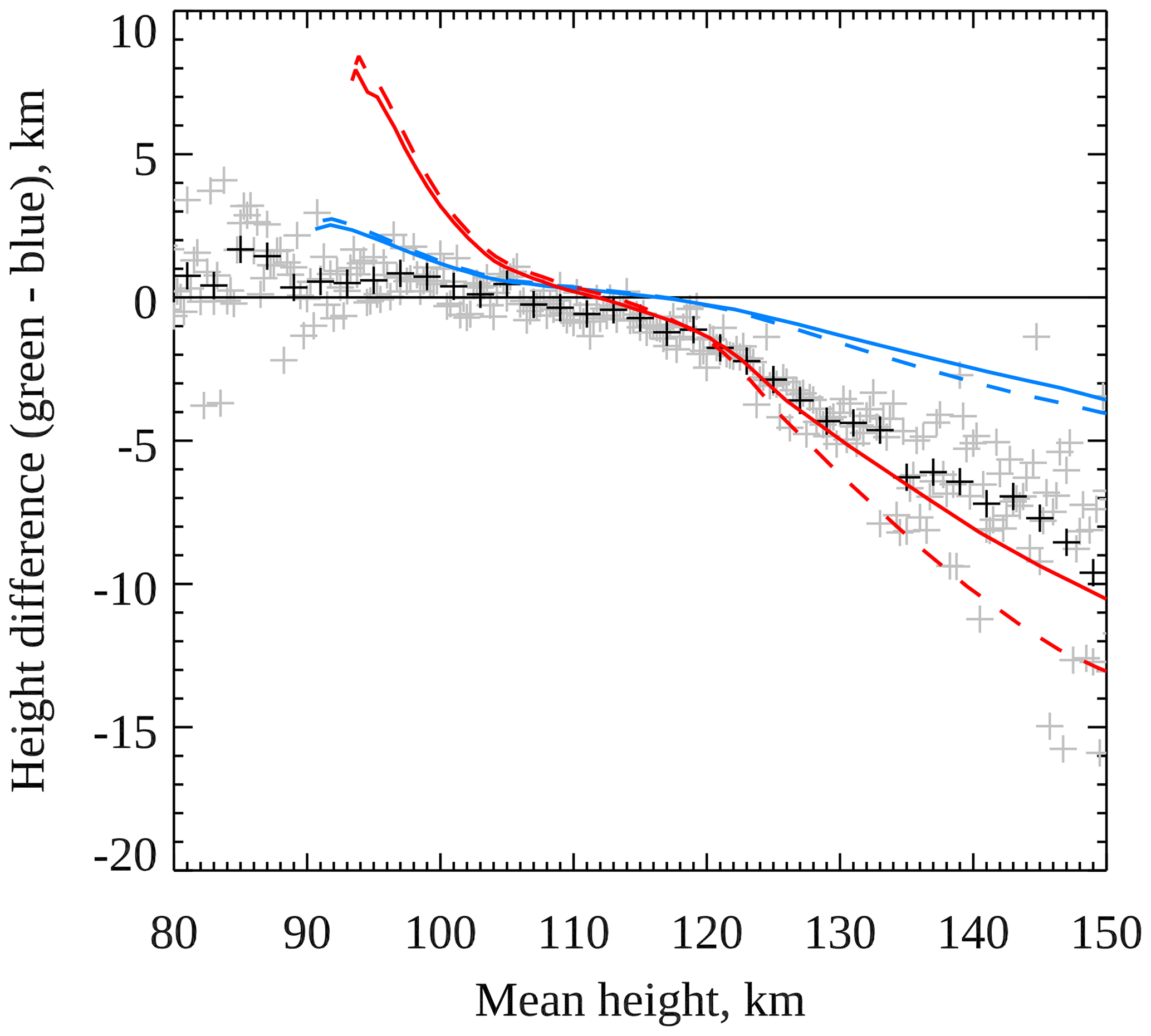
Figure 9 Observed and modelled difference in height between the green 557.7 nm and blue 427.8 nm emissions as a function of their mean height. Observations are shown as plus symbols. Grey symbols show the average height difference over all observations with the same mean height (to the nearest 0.25 km). Black symbols show the same but where observations have been binned into 2 km wide bins of mean height (reproduced from Fig. 4). The blue and red curves show the model results for Gaussian- and Maxwellian-shaped electron precipitation spectra, respectively, where the model is run for 12 s (steady state, solid curves) or for 3 s (dashed curves).

The model also does a good job of quantitatively reproducing the observations. For a quantitative comparison we return to the examination of how the height difference between the two emissions varies as a function of mean peak emission height, introduced earlier in Fig. 4 and continued here in Fig. 9, to avoid the need to estimate the electron precipitation energy during the observations. Since the peak emission heights are measured in the camera data to the nearest 0.5 km, the mean of the coincident green and blue peak heights always has a value divisible by 0.25 km. The average observed height differences calculated for possible values of the mean height (i.e. every 0.25 km) are shown as grey plus symbols in Fig. 9. The average height difference calculated for 2 km wide bins of mean height, as shown as white plus symbols in Fig. 4, is reproduced with black plus symbols in Fig. 9. These black points show less scatter than the grey points since more observations are included in the calculation of each one. The solid blue and red curves represent the model results described above for Gaussian and Maxwellian spectra, respectively, and are essentially the same as the black curves shown in Figs. 7 and 8 with the abscissae transformed from electron precipitation energy to mean height. The dashed blue (Gaussian) and red (Maxwellian) curves show the results of running the model for only 3 s instead of 12 s. We consider the results separately for low- and high-energy precipitation below.

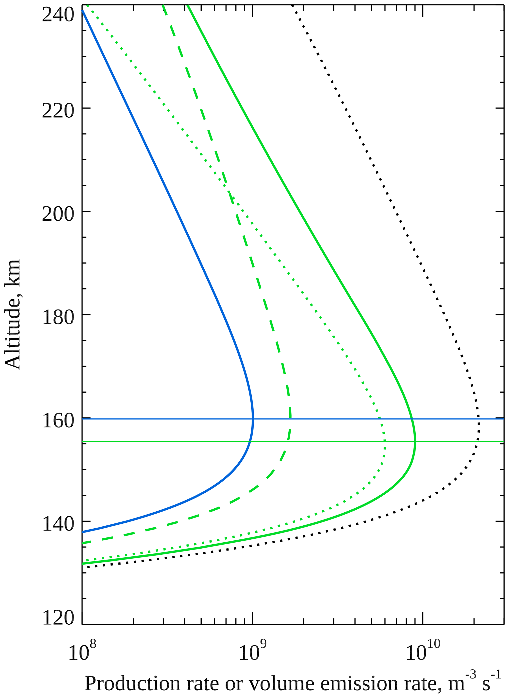
Figure 10 Modelled volume emission rate height profiles of the 427.8 nm blue line (solid blue) and 557.7 nm green line (solid green) using a 900 eV Gaussian electron precipitation spectrum. The horizontal lines mark the peaks of the volume emission rate profiles. Also shown are the production rates of O(¹S) by energy transfer from N₂(A) (dotted green) and electron impact on O (dashed green) and the production rate of N₂(A) (dotted black).

5.1 Low-energy electron precipitation

To understand the observations and model results we examined the altitude profiles of the relevant reaction rates and number densities. Figure 10 shows the modelled volume emission rate altitude profiles of the 557.7 and 427.8 nm emissions as solid green and blue lines, respectively, for a Gaussian electron precipitation spectrum at 900 eV. The production rates of O(¹S) by the two dominant sources during low-energy precipitation, energy transfer from N₂(A) (Reaction R5) and electron impact excitation (Reaction R1), are shown as dotted and dashed green lines, respectively, and the production rate of N₂(A) is shown as a dotted black line. The peak emission heights of the two emissions are marked with horizontal lines. This figure highlights that at low electron precipitation energies, the ionisation of N₂ peaks at a higher altitude than the production of O(¹S) by energy transfer from N₂(A), which could seem counter-intuitive given that the ionisation energy of N₂ is greater than the threshold energy for excitation to N₂(A). The reason is that the N₂(A)+O energy transfer rate depends on the product of the atomic O number density and N₂(A) number density. Since the O number density decreases to higher altitudes, this product peaks at lower altitude than the N₂(A) density and ${\mathrm{N}}_{\mathrm{2}}^{+}$ production rate. Ultimately this is why the blue 427.8 nm emission peaks above the green 557.7 nm emission.

The model results using a Maxwellian electron spectrum best match the average observations above 110 km (dashed red curve in Fig. 9). However, the observations show broad variation in the height difference for high mean heights (see Fig. 4), which is reproduced by varying the model run time and electron spectrum shape. Running the model for a shorter time period means that a steady state is not achieved, in particular regarding the N₂(A) and O(¹S) number densities, and the spread of observed height differences may reflect the spatial and temporal dynamics of the auroral precipitation.

5.2 High-energy electron precipitation

For both Gaussian and Maxwellian electron spectra, the model produces a green peak emission height above the blue height (i.e. positive height difference in Fig. 9) for high-energy precipitation where the mean peak emission height is below about 110 km, with the height difference increasing away from the observations with increasing energy of precipitation. The median F10.7 index at times where both emissions peak below 105 km is within 0.1 standard deviations of the median F10.7 index for other times, indicating that the low-altitude emissions are primarily a result of energetic precipitation, rather than a contracted atmosphere. At these high energies, the Gaussian spectra produce model results that are more consistent with observations than those for the Maxwellian spectra, which may be an indication that more energetic precipitation (above about 4 keV) is typically more Gaussian in spectral shape, but neither spectral shape reproduces the observations well at the lowest altitudes. The mean height peaked below 110 km in 35 % of our observations.

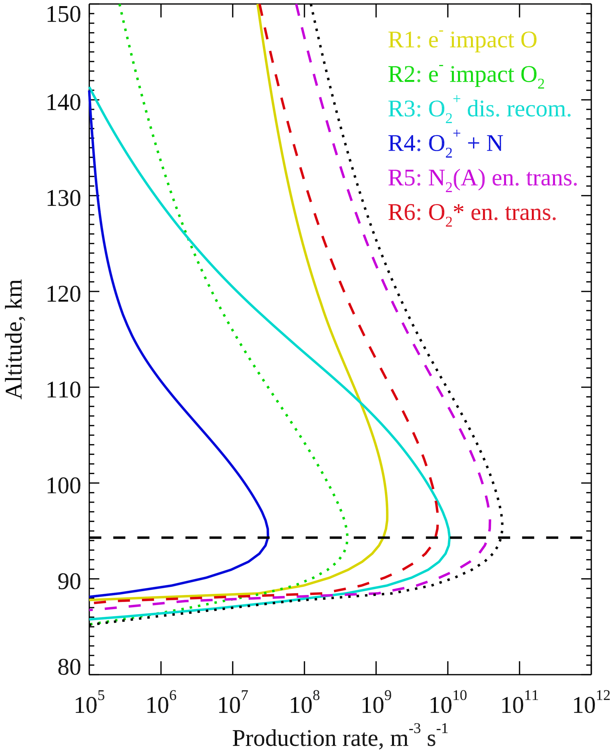
Figure 11 Modelled production rate profiles of O(¹S) after 12 s of Gaussian electron precipitation at 25 keV. The reactions producing O(¹S) are listed in Table 2. The rates of Reactions (R1), (R2), (R3), (R4), (R5), and (R6) are plotted by solid yellow, dotted green, solid cyan, solid blue, dashed magenta, and dashed red lines, respectively. The total production rate of O(¹S) is shown by the dotted black line. The horizontal dashed line marks the peak height of the blue 427.8 nm emission.

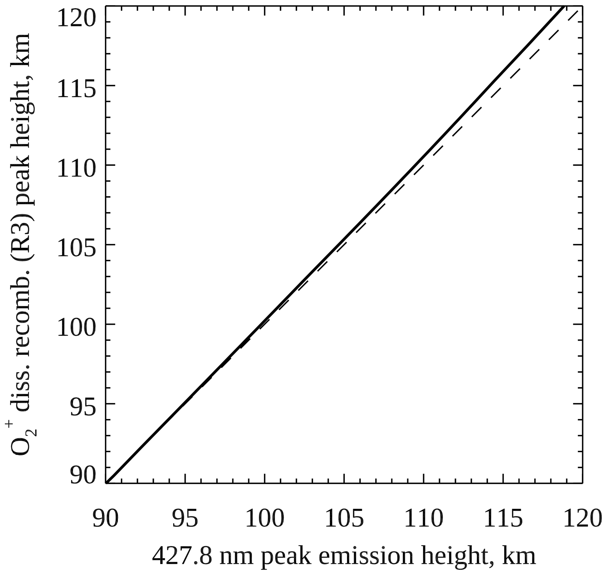
Figure 12 Modelled peak height of the production rate of O(¹S) by dissociative recombination of ${\mathrm{O}}_{\mathrm{2}}^{+}$ (Reaction R3) against the blue 427.8 nm peak emission height (electron impact ionisation of N₂). The dashed line marks where the two rates would be equal.

Figure 11 shows altitude profiles of the six O(¹S) production mechanisms included in the model, for a Gaussian electron spectrum at 25 keV with a flux of 20 mW m⁻² running for 12 s. Auroral electron impacts on O (Reaction R1) and O₂ (Reaction R2) are shown as solid yellow and dotted green lines, respectively. Dissociative recombination of ${\mathrm{O}}_{\mathrm{2}}^{+}$ (Reaction R3) is shown as a solid cyan line, and Reaction (R4) between ${\mathrm{O}}_{\mathrm{2}}^{+}$ and N is shown as a solid blue line. Energy transfer from N₂(A) (Reaction R5) and ${\mathrm{O}}_{\mathrm{2}}^{*}$ (Reaction R6) is shown as dashed magenta and red lines, respectively. The dotted black line shows the total production rate of O(¹S), and the horizontal dashed line shows the peak height of the blue 427.8 nm emission. Of the six mechanisms, dissociative recombination of ${\mathrm{O}}_{\mathrm{2}}^{+}$, electron impact on O₂, and ${\mathrm{O}}_{\mathrm{2}}^{+}+\mathrm{N}$ all peak at the same height as the 427.8 nm emission. Figure 12 shows the ${\mathrm{O}}_{\mathrm{2}}^{+}$ dissociative recombination rate peak height plotted against the 427.8 nm peak emission height for Gaussian electron precipitation. The dashed line represents equal rates (y=x). The two rates peak at very similar altitudes through the E-region ionosphere, especially below 105 km.

O'Neil et al. (1979) used rocket-based optical observations of artificial aurora with modelling to conclude that dissociative recombination of ${\mathrm{O}}_{\mathrm{2}}^{+}$ (Reaction R3) is the dominant production mechanism of O(¹S) below 96 km, with energy transfer from N₂(A) (Reaction R5) dominating from 100 km to 116 km (the upper altitude limit of their measurements). Our work and observations support this conclusion, except that in our model the production of O(¹S) by dissociative recombination of ${\mathrm{O}}_{\mathrm{2}}^{+}$ is too slow compared to energy transfer from N₂(A) at low altitudes. We currently do not have a solution to this discrepancy, but in the following subsections we consider whether the modelled Reaction (R3) is too slow, Reaction (R5) is too fast, or there is an O(¹S) production mechanism missing from the Southampton ionospheric model.

5.2.1 O(¹S) from dissociative recombination of O${}_{\mathrm{2}}^{+}$

For dissociative recombination of ${\mathrm{O}}_{\mathrm{2}}^{+}$ the model uses a quantum yield of O(¹S) of 0.05 from Kella et al. (1997), with a temperature dependent rate coefficient from the review by Sheehan and St.-Maurice (2004). The rate coefficient is given by

$$\begin{array}{}\text{(1)}& \mathrm{1.95}\times {\mathrm{10}}^{-\mathrm{13}}(T_{\mathrm{e}}/\mathrm{300}{)}^{-\mathrm{0.70}}{\mathrm{m}}^{\mathrm{3}}{\mathrm{s}}^{-\mathrm{1}},\end{array}$$

where T_e is the electron temperature in kelvin. This rate coefficient was measured by Mehr and Biondi (1969) and agrees exactly with that found by Alge et al. (1983). Peverall et al. (2001) found a rate 23 % larger (with the same temperature dependence), although their quantum yield of O(¹S) was lower than that of Kella et al. (1997) (but with an electron energy dependence). There is little evidence in the literature for a substantially larger rate coefficient than this. Abreu et al. (1983) used observations of airglow to determine the quantum yield of O(¹S) and found values between 0.09 and 0.23, with a dependence on the ratio of electron density to O density (greater yield with larger ratio) from which they inferred a dependence on the vibrational excitation of the ${\mathrm{O}}_{\mathrm{2}}^{+}$. This vibrational dependence was also found in laboratory measurements by Petrignani et al. (2005), who found quantum yields of 0.06, 0.14, and 0.21 for vibrational levels v=0, 1, and 2 respectively. The Southampton model does not track individual vibrational levels of ${\mathrm{O}}_{\mathrm{2}}^{+}$, but the O(¹S) quantum yield could be increased from 0.05 to reflect the average value across an assumed vibrational distribution. Using a value of 0.2 in the model does improve the fit to observations below 110 km, although the modelled height difference is still larger than observations below 100 km.

The production rate of O(¹S) through dissociative recombination (Reaction R3) could also be underestimated as a consequence of an underestimated ${\mathrm{O}}_{\mathrm{2}}^{+}$ density, either because the ionisation rate is too slow or because the O₂ mixing ratio is too low. We note that the N₂ and O densities were reduced in the latest version of MSIS, but Emmert et al. (2021) conclude that the O₂ density is more uncertain due to an absence of suitable data in the middle thermosphere.

5.2.2 O(¹S) excited by energy transfer from N₂(A)

The production of O(¹S) through energy transfer from N₂(A) depends not only on the rate of the energy transfer itself, but also on the production and loss rates of the long-lived N₂(A). Production of N₂(A) is by electron impact excitation, but cascading from the B³Π_g state via the First Positive transition is the dominant production mechanism, and B³Π_g is itself fed by cascading from the C³Π_u and W³Δ_u states. Since these cascade transitions are prompt, to calculate production of N₂(A), the model sums electron impact excitation to the $A^{\mathrm{3}}{\mathrm{\Sigma }}_{\mathrm{u}}^{+}$, B³Π_g, and W³Δ_u states, with half of the excitation to the C³Π_u state also included. For N₂ electron impact excitation, the model uses the “J05M09” cross sections of Yonker and Bailey (2020), which gave a marginally better agreement with our observations than the cross sections of Itikawa (2006). N₂(A) is lost through quenching by O₂ and O with rates from Gattinger et al. (1996) and Piper (1982), respectively, as well as emission in the Vegard–Kaplan (A–X) band system (Einstein coefficient 0.38 s⁻¹, from Piper, 1993). Quenching by O₂ can indirectly lead to production of O(¹S) via ${\mathrm{O}}_{\mathrm{2}}^{*}$, through Reaction R6, although ${\mathrm{O}}_{\mathrm{2}}^{*}$ is also quenched. During energetic precipitation ($>\sim$ 10 keV), O(¹S) production by energy transfer from N₂(A) peaks above the ${\mathrm{N}}_{\mathrm{2}}^{+}$ 1 N (427.8 nm) emission since quenching of N₂(A) by O₂ at low altitudes raises the peak height of the N₂(A) number density. Below the mesopause, the O(¹S) production by energy transfer also falls off with the O number density.

For the N₂ energy transfer reaction (R5), we use the rate coefficient ($\mathrm{2.8}\times {\mathrm{10}}^{-\mathrm{17}}$ ${\mathrm{m}}^{\mathrm{3}}{\mathrm{s}}^{-\mathrm{1}}{\mathrm{molecule}}^{-\mathrm{1}}$) and O(¹S) quantum yield (0.75) of Piper (1982). The larger (by 25 %) rate coefficient of Thomas and Kaufman (1985) was used by Yonker and Bailey (2020), but using that coefficient in our model would increase the dominance of energy transfer from N₂(A) in the production of O(¹S) at low altitudes and would therefore make the match to observations worse. Hill et al. (2000) proposed a temperature-dependent rate coefficient for Reaction (R5), although Yonker and Bailey (2020) argued against a temperature dependence. Replacing the rate from Piper (1982) with that from Hill et al. (2000) led to a marginal improvement in the match between the model and observations at high electron precipitation energies but made the match considerably worse at high altitudes for low-energy precipitation.

5.2.3 Possible pathways for producing O(¹S) missing from the Southampton ionospheric model

Besides overestimated or underestimated rates, there may be sources of O(¹S) completely missing from the Southampton ionospheric model which could explain the discrepancy with our observations at the lowest altitudes. We briefly consider two possibilities here, represented by

$$\begin{array}{}\text{(R7)}& {\displaystyle }\mathrm{N}{(}^{\mathrm{2}}D)+\mathrm{NO}\to {\mathrm{N}}_{\mathrm{2}}+\mathrm{O}\text{(R8)}& {\displaystyle }{\mathrm{O}}_{\mathrm{2}}+e^{-}\to {\mathrm{O}}^{+}+\mathrm{O}+\mathrm{2}{e}^{-}.\end{array}$$

Reaction (R7) is thought to occur in the upper atmosphere (e.g. Barth, 1992), and the production of O(¹S) is energetically allowed, but the quantum yield of O(¹S) is not yet known (Fox and Hać, 2018). The Southampton model uses a rate coefficient for this reaction from Lin and Kaufman (1971), with all O being produced in the ground state. Similarly, electron impact dissociative ionisation of O₂ in which one of the products is O⁺ (Reaction R8) is also included in the model (as a distinct reaction to Reaction R2) but not as a source of O(¹S). No branching ratio for the production of O(¹S) via Reaction (R8) is available.

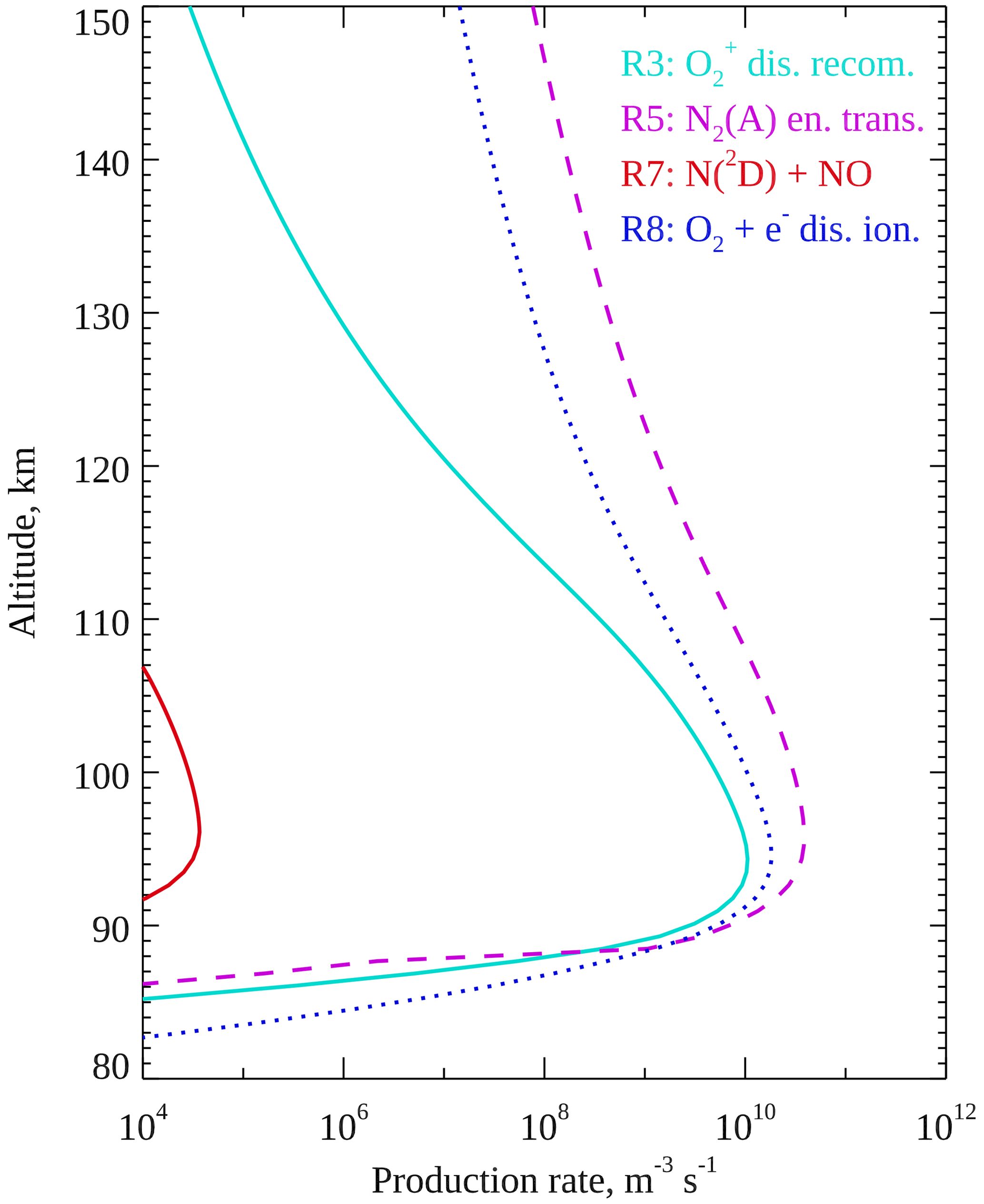
Figure 13 Modelled rate profiles after 12 s of Gaussian electron precipitation at 25 keV. The rates of Reactions (R3), (R5), (R7) and (R8) are plotted by solid cyan, dashed magenta, solid red, and dotted blue lines, respectively. Reactions (R3) and (R5) are production of O(¹S) and are exactly as plotted in Fig. 11. Reactions (R7) and (R8) are production of O in any state.

Modelled altitude profiles of the rates of Reactions (R7) and (R8) are plotted in Fig. 13 by solid red and dotted blue lines, respectively, for a Gaussian electron precipitation spectrum at 25 keV with a flux of 20 mW m⁻² running for 12 s. Reaction (R3) (solid cyan) and Reaction (R5) (dashed magenta) are reproduced from Fig. 11 for comparison. The rate of Reaction (R7) is several orders of magnitude too small to have a significant effect on the auroral peak emission altitude and peaks at higher altitude than ${\mathrm{O}}_{\mathrm{2}}^{+}$ dissociative recombination, so we discount that reaction. In contrast, the rate of Reaction (R8) is approximately twice the rate of ${\mathrm{O}}_{\mathrm{2}}^{+}$ dissociative recombination (Reaction R3) at the peak and therefore may be significant if the quantum yield of O(¹S) is not too low.

Further work is required to evaluate the possible contributions of these, and other, mechanisms to the production of O(¹S) in the aurora, ideally including experimental determination of the relevant rate coefficients, cross sections, and quantum yields.

6 Conclusions

The typical peak emission height of both green 557.7 nm aurora and blue 427.8 nm aurora is about 114 km (113.8 km for green and 113.5 km for blue, according to our large set of observations from Lapland in 2000–2007). When the emissions peak below this typical height they peak at a very similar height, with the green very slightly (∼ 1 km) above the blue, on average. When they peak at higher altitudes, the blue usually peaks above the green.

During low-energy electron precipitation, the dominant mechanism producing the O(¹S) responsible for the green emission is energy transfer from N₂(A). The green line peaks at lower altitude than the blue line because the production rate of O(¹S) (green line) depends on the product of N₂ and O number densities, which both decrease with higher altitude, whereas electron impact production of ${\mathrm{N}}_{\mathrm{2}}^{+}$ (blue line) depends on the number density of only N₂. The height difference between the two emissions is sensitive to the primary electron spectrum shape as well as the duration of the precipitation but on average reaches about 10 km when the green line peaks at 145 km.

During high-energy precipitation, the dominant mechanism producing O(¹S) at low altitudes must not be energy transfer from N₂(A). Dissociative recombination of ${\mathrm{O}}_{\mathrm{2}}^{+}$ seems the most likely candidate, but in that case the Southampton ionospheric model underestimates the rate of this process or overestimates the rate of energy transfer from N₂(A) to O(¹S), or there is a combination of both. We tentatively suggest that electron impact dissociative ionisation of ${\mathrm{O}}_{\mathrm{2}}^{+}$ in which O⁺ is one of the fragments may be an additional source of O(¹S) missing from models, although its inclusion may not be enough to bring the Southampton model in line with our observations, and other mechanisms may also be missing.

A comparison between our model results and observations suggests that the auroral electron precipitation energy spectrum is typically Gaussian when the characteristic energy is above about 4 keV but closer to Maxwellian at lower characteristic energies.