the Creative Commons Attribution 4.0 License.
the Creative Commons Attribution 4.0 License.
 | 31 Jan 2022
Estimating ion escape from unmagnetized planets
We propose a new method to estimate ion escape from unmagnetized planets that combines observations and models. Assuming that upstream solar wind conditions are known, a computer model of the interaction between the solar wind and the planet is executed for different ionospheric ion production rates. This results in different amounts of mass loading of the solar wind. We then obtain the ion escape rate from the model run that best fits observations of the bow shock location. As an example of the method, we estimate the heavy-ion escape from Mars on 1 March 2015 to be 2×1024 ions s−1, using a hybrid plasma model and observations by the Mars Atmosphere and Volatile Evolution (MAVEN) and Mars Express (MEX) missions. This method enables studies on how escape depends on different parameters as well as studies on escape rates during extreme solar wind conditions; moreover, the technique is applicable to studies of escape in the early solar system and at exoplanets.
- Article
(909 KB) - Full-text XML
- BibTeX
- EndNote


Ion escape to space is important for the evolution of planetary atmospheres. Neutral atoms or molecules in the upper parts of the atmosphere can be ionized by factors such as ultraviolet (UV) photons, charge exchange, and electron impacts. The newly created ion can then be energized by electric fields and transported away by the stellar wind, overcoming gravity, resulting in atmospheric loss.
For planets in our solar system, we can observe the present-day escape of planetary ions by directly observing the ion flux near a planet. This is done using an ion detector on a spacecraft and gives us the flux of ions along the trajectory of the spacecraft. As the flux of escaping ions is highly variable both temporally and spatially, accurately estimating the escape of ions can require observations over many years to get an average escape rate. Investigating how the escape rate of ions depends on different parameters (e.g., upstream solar wind conditions) is even more difficult due to the large amounts of observations needed to get sufficient statistics.
Another way of estimating ion escape rates is to use computer models of the solar wind interaction with a planet. An advantage of models compared with observations is that the full three-dimensional escape is obtained at every instance. In addition, there are no limitations with respect to sensitivity, energy range, or field of view, in contrast to the limitations on observations. However, accurately estimating ion escape requires that the model contains all of the important physical processes in sufficient detail. It is questionable if this is the case at present.
Here, we propose an alternative method of estimating ion escape that uses both observations and computer models. Instead of directly observing the escaping ions, we use observations of other plasma quantities near the planet. We then employ a parameterized model and find the set of model parameters that gives the best fit between the model and the observations. The model escape rate for the best fit parameters gives us an estimate of the ion escape rate.
This approach allows us to use data sets traditionally not used for ion escape estimates, such as magnetic field and electron observations. We can also estimate the escape rate from a very small set of observations, during one orbit of a spacecraft around a planet or during one flyby of a planet.
To illustrate this general method, we estimate the escape rate of ions from Mars during one bow shock crossing of the Mars Atmosphere and Volatile Evolution (MAVEN) spacecraft (Jakosky et al., 2015) using magnetic field observations of the bow shock location, observations of the upstream solar wind conditions, and a hybrid plasma model. We also use Mars Express (MEX) (Barabash et al., 2007) observations of electrons to verify our findings.
The location and shape of the Martian bow shock have been the topic of many observational studies that have aimed to establish where the bow shock is located and its controlling parameters. Recently Hall et al. (2016) found a seasonal dependence of the bow shock location and, later, also a solar cycle dependence (Hall et al., 2019). The seasonal dependence should be due to the changing distance of Mars from the Sun; however, it is not straight forward to deduce if it is due to changing solar wind pressure or changing UV insolation, as both scale in the same way with distance from the Sun. Moreover, both the solar wind and the UV insolation change over a solar cycle. Regarding the effect of crustal magnetic fields on the bow shock location, Gruesbeck et al. (2018) found such a dependence; furthermore, a modeling study by Fang et al. (2017) found that a large part of the variability in escape may be due to the crustal fields, reducing and enhancing escape, depending on the location. Regarding the shape of the bow shock, Vignes et al. (2002) found that it is furthest away from the planet in the hemisphere in the direction of the solar wind convective electric field.
However, it has been noted that, apart from the upstream solar wind conditions, the factor controlling the location of the shock is the amount of mass loading of the solar wind by ionospheric ions. This was noted for Venus by Alexander and Russell (1985) and later for Mars by Vignes et al. (2002) and Mazelle et al. (2004). The UV flux, atmospheric state, ionospheric chemistry, magnetic anomalies, and similar factors will all affect the location of the bow shock, although only indirectly through the amount of mass loading. Therefore, given upstream solar wind conditions, we should be able to use the amount of mass loading as a free parameter when modeling the location of the bow shock.
The algorithm presented in this paper is general and can be applied to any model of the interaction between Mars and the solar wind. Here, to illustrate the method, we use a very simple hybrid model.
We now describe the hybrid plasma solver used; the adaptation for Mars; the parameters used; the observations of magnetic field, ions, and electrons used; and, finally, the algorithm to estimate ionospheric ion escape.
2.1 Hybrid model
In the hybrid approximation, ions are treated as particles, and electrons are treated as a massless fluid. The trajectories of the ions are computed from the Lorentz force, given the electric and the magnetic fields. The electric field is
where ρI is the ion charge density, JI is the ion current density, pe is the electron pressure, and η is the resistivity. The current is computed from , where is the magnetic constant.
Faraday's law is then used to advance the magnetic field in time:
Further details on the hybrid model used here, the discretization, and the handling of vacuum regions can be found in Holmstrom et al. (2012).
2.2 Mars model
In the hybrid simulation domain, Mars is modeled as a resistive sphere, of radius R, centered at the origin, where all ions that hit the obstacle are removed from the simulation.
The ionosphere is represented by the production of a single species of ions according to an analytical Chapman ionospheric profile (Holmstrom and Wang, 2015), where the production rate of ions is given by
Here, h [m] is the height above the planet surface; χ [rad] is the solar zenith angle (SZA); p [m−3 s−1] is the maximum production along the sub-solar line, at height h0 [m]; and H [m] is the scale height. Ions are then randomly placed according to this production function and are also given a random thermal velocity corresponding to a temperature of 200 K.
We note that the ion production is a free parameter in such a model. This is in contrast to models that self-consistently include ionospheric chemistry and a neutral atmosphere (Brecht et al., 2016). Usually this free parameter is seen as a limitation of the model; however, here, we use this as an advantage in order to find a best fit to observations. This means that the exact processes in the ionosphere that produce the ions or how they are transported to the top of the ionosphere is not important.
Regarding the composition of escaping ionospheric ions, a study by Carlsson et al. (2006) based on MEX observations found flux ratios of O O and CO O. Later, Rojas-Castillo et al. (2019) estimated that O O. Using MAVEN data, Inui et al. (2019) found a flux ratio of O O and reported that CO contributed less than 10 % to the total heavy-ion flux. In summary, observations indicate that the flux of escaping O+ and O ions are of similar magnitude and that the CO flux is not significant.
As the code used here only handles one single-charged ionospheric ion species, we carry out separate simulation runs using O+ and O to investigate the effects of composition on the ion escape rate estimates. Note also that there is no neutral H or O corona in the model. Thus, those populations of exospheric pick-up ions are missing. This means that the mass loading due to the corona is missing in the simplified model that we use. The total mass loading can be compensated for by more ions from the ionospheric source; however, in reality, the spatial distribution would be different. We also do not include any alpha particles in the solar wind, which should have some effect on the solar wind interaction.
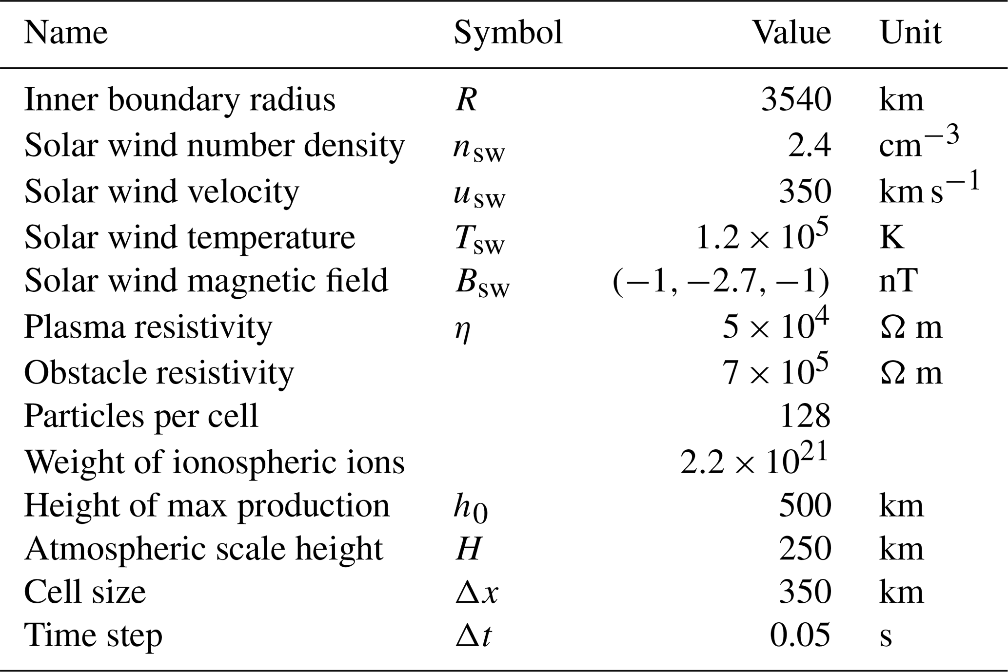
2.3 Model parameters
The coordinate system used is MSO (Mars Solar Orbital) coordinates with the solar wind flowing along the −x axis, with density nsw, speed vsw, and temperature Tsw. The upstream interplanetary magnetic field is Bsw. The computational grid has cubic cells of size Δx, and the time step is Δt. The computational domain is , , and km. On the upstream boundary, after each time step, we insert solar wind protons so that the number of particles per cell there is constant. In the y and z directions, we have periodic boundary conditions. The produced ionospheric ions have a weight (how many real ions they represent) that is chosen such that the weight is similar to that of the solar wind protons. The model parameters and their values are listed in Table 1.
2.4 Observations
We use MAVEN magnetic field (Connerney et al., 2015; Dunn, 2021) and ion (Halekas et al., 2017) observations to determine upstream conditions and bow shock location. The orbit is chosen such that the solar wind conditions are steady (so that the conditions should be unchanged while MAVEN is inside the bow shock) when we do not have observations of the solar wind. This also allows us to use a simulation that does not have time-dependent upstream solar wind conditions. To verify our results, we also use MEX observations of electrons (Lundin et al., 2005; Frahm et al., 2006) to locate bow shock crossings. The upstream solar wind parameters are listed in Table 1.
2.5 Algorithm
We now describe the algorithm (illustrated in Fig. 1) for estimating the escape of ionospheric ions from observations of the upstream solar wind and the location of the bow shock:
-
We start with an observed state of the upstream solar wind – the magnetic field and the solar wind density, velocity, and temperature.
-
We then carry out several runs of the hybrid model for these upstream solar wind conditions, using different ionospheric ion production rates.
-
Next, we find the simulation run that has a bow shock location that best corresponds to the observed location. This could be done quantitatively (e.g., by a least squares fit), but here we visually compare the simulations and the observations.
-
The escape for the best fit simulation run is then computed, and this will be our estimate of the escape rate of ionospheric ions at the time of the bow shock observation.
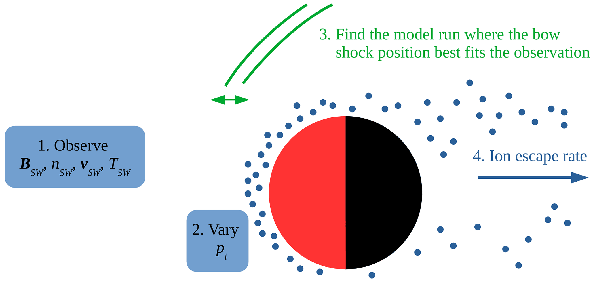
Figure 1An illustration of the algorithm to estimate the ion escape rate. The Sun is to the left, and Mars is the red and black disk. Using fixed upstream solar wind conditions from observations in the hybrid model, we vary the ionospheric heavy-ion (blue dots) production rate for different simulation runs. The bow shock location (green lines) in each simulation run is then compared to the observed bow shock location. The estimated escape rate corresponds to that of the simulation run that best fits the bow shock location.
As an example of the proposed algorithm, we performed 10 simulations with the production rates [cm−3 s−1]. In Fig. 2, we present a comparison of MAVEN observations and two hybrid runs (R1 and R2) with an O+ ionosphere and different ion production rates that were judged to best fit the observations. We see that there is a fairly good agreement between the models and the observations at the bow shock and in the magnetosheath. However, closer to the planet, in the induced magnetosphere, the agreement is not as good. The magnetic field is much larger and more variable than in the model. This is not surprising because we have a model with a very simplified ionosphere, no magnetic anomalies, and low spatial resolution. Moreover, in the magnetosphere, the proton velocities in the model are much higher than observed. However, the proton density is very small, close to zero, in much of this region, as observed and as shown in the simulations. Near the exit from the induced magnetosphere, the observed density is larger than in the simulations, resulting in a similar dynamic pressure. Furthermore, the variability of Bz in the magnetosheath is smaller in the models than in the observations.
As expected and as seen when comparing the two model runs, the location of the bow shock moves outward when the ionospheric ion production is increased, resulting in a larger mass loading.
The escape rate never reaches a steady state due to the intrinsic variability of the induced magnetosphere. Therefore, we determine the escape rate by averaging the flux of ionospheric ions along −x in the simulation domain, from km to the outflow boundary. We then average these computed escape values over time, between 200 and 590 s, with a time step of 10 s.
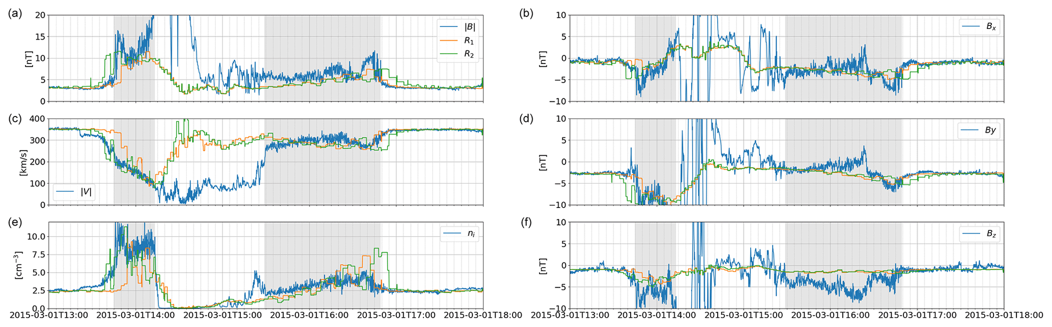
Figure 2A comparison of MAVEN observations (blue) with two O+ model runs (R1 in orange and R2 in green) at 490 s. Panels (a), (c), and (e) show the magnetic field magnitude, proton velocity, and proton number density, respectively. Panels (b), (d), and (f) show the three respective magnetic field components (Bx, By, and Bz) in MSO coordinates. The location of the magnetosheath as seen from the observations is also indicated in gray. Thus, the induced magnetosphere is between the two gray regions.
Table 2The different best fit simulation runs, the ionospheric ion species, the maximum ionospheric production rates, and the resulting escape rates.
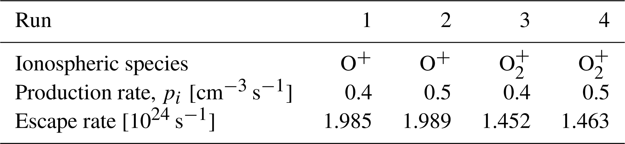
In Table 2, we show the results of simulation runs R1–R4, performed for O+ and O ionospheres with different ion production rates. For the best fit runs using O+, the approximate escape rate is 2.0×1024, whereas it is 1.5×1024 s−1 for O. As we have a mixture of the two ion species in reality, the escape rate should be between these values, and we can estimate the actual escape as 2×1024 s−1.
We can note how the escape rate for the best fit simulation runs depends on the species of the escaping ionospheric ions. The best fit has 25 % less escaping O ions compared with O+. It is not, however, directly proportional to the total mass of the escaping ions; in that case, we would expect a 50 % reduction. Thus, it is not only the amount of mass loading that characterizes the best fit, the dynamics of the escaping ions is also important.
Looking at the escape rate in Table 2 for the same species but for different ion production rates, we see that it is weakly dependent on the production rate. The two best fit runs in Fig. 2 have less than a 1 % difference in the escape rate.
To verify the location of the bow shock in the two best fit model runs, we also use MEX observations of the bow shock in electron data. In Fig. 3, we plot the proton number density from the same two hybrid runs as in Fig. 2, although now along the MEX orbit, along with the location of the bow shock crossings observed by MEX. The agreement is fairly good, even if the observed bow shock is a few minutes earlier than that seen in the model runs. This corresponds to a distance of a few hundred kilometers, which is comparable to the simulation grid cell size. One reason for this could be that we have not used an aberrated solar wind velocity (it flows along the −x axis). This should result in a tilt of the whole magnetosphere and bow shock.

Figure 3The proton number density along the MEX orbit for the two best fit simulation runs (R1 in orange and R2 in green), at 490 s of simulation time. The blue vertical lines show the two bow shock crossings seen in MEX electron data.
For our example case, we found an escape rate of 2×1024 ions s−1. This is in the range of recently published estimates for the escape rate at Mars (Ramstad et al., 2015; Brain et al., 2015; Dong et al., 2017).
An assumption is that, given upstream conditions, the mass loading determines the bow shock location. Although we find an escape rate for a single orbit that matches observed escape rates, this assumption needs to be tested in more detail. An ongoing investigation is to apply the method to a large number of orbits and verify that the model-estimated escape rates are consistent with observed escape rates.
The proposed method is directly applicable to unmagnetized planets. For magnetized planets, the bow shock location is mainly determined by the upstream solar wind and the strength of the dipole field. Escape at magnetized planets occurs in the cusp regions; how this affects the bow shock location as well as if the presented method could be adapted to magnetized planets would need further investigation.
The bow shock location has been found to depend on the location of the magnetic anomalies relative to the solar wind flow (Fang et al., 2017). It is unclear if this is because the fields “push out” the boundaries or because the fields increase ion escape. The latter may not require crustal fields in the model used in our algorithm, as the parameter that we vary is the amount of ions near Mars available to escape. If the crustal fields in a specific geometry enhance escape, this will be captured in the algorithm because the best fit bow shock will be further out; in contrast, if the crustal fields in a specific geometry depress escape, the bow shock will be closer to the planet.
We used a hybrid plasma model in the algorithm. It would, however, be possible to use another type of plasma model, such as a magnetohydrodynamic (MHD) model, that can predict the location of the bow shock for different amounts of mass loading by ionospheric ions, given upstream solar wind conditions.
In the past, ion escape has been estimated either by computer models or from observations. Models have the problem that every physical process has to be present in the model. In contrast, observations suffer from variability, requiring the averaging of data over years or even decades. The method proposed here uses a model and observations together. In this way, we overcome the difficulties of each approach. We then get an estimate of the escape using just one observation. A model is used to estimate a global property (ion escape) from a local observation (bow shock location). As we use a model, there are not the physical limitations – in terms of energy coverage and field of view – that are present in observations. In particular, low-energy escaping ions are difficult to observe.
This opens up the possibility of estimating escape during flybys of unmagnetized planets, in the past and in the future. It also allows for the estimation of escape twice per orbit given only a magnetometer and an ion detector. This enables detailed studies on how the escape depends on different parameters, which has been difficult in the past due to the years of observations needed to collect enough statistics. It also makes the study of escape during transient events, like extreme solar wind conditions, possible, which is something that is important for studies on escape in the past as well as escape at exoplanets.
The MAVEN data used in this work, ion data from the Solar Wind Ion Analyzer (SWIA) instrument and magnetic field data from the magnetometer (MAG), are available from the NASA Planetary Data System (PDS) at https://pds-ppi.igpp.ucla.edu/search/view/?f=null&id=pds://PPI/maven.insitu.calibrated/data/2015/03 (Dunn, 2021). The ASPERA-3 electron data used, from the electron spectrometer (ELS), are available from https://pds-ppi.igpp.ucla.edu/search/view/?id=pds://PPI/MEX-M-ASPERA3-3-RDR-ELS-EXT5-V1.0 (Lundin et al., 2005).
The contact author has declared that there are no competing interests.
Publisher’s note: Copernicus Publications remains neutral with regard to jurisdictional claims in published maps and institutional affiliations.
Computing resources used in this work were provided by the Swedish National Infrastructure for Computing (SNIC) at the High Performance Computing Center North (HPC2N), Umeå University, Sweden. The software used in this work was in part developed by the DOE NNSA-ASC OASCR Flash Center at the University of Chicago.
This paper was edited by Peter Wurz and reviewed by one anonymous referee.
Alexander, C. J. and Russell, C. T.: Solar Cycle Dependence of the Location of the Venus Bow Shock, Geophys. Res. Lett., 12, 369–371, https://doi.org/10.1029/GL012i006p00369, 1985. a
Barabash, S., Lundin, R., Andersson, H., Brinkfeldt, K., Grigoriev, A., Gunell, H., Holmström, M., Yamauchi, M., Asamura, K., Bochsler, P., Wurz, P., Cerulli-Irelli, R., Mura, A., Milillo, A., Maggi, M., Orsini, S., Coates, A. J., Linder, D. R., Kataria, D. O., Curtis, C. C., Hsieh, K. C., Sandel, B. R., Frahm, R. A., Sharber, J. R., Winningham, J. D., Grande, M., Kallio, E., Koskinen, H., Riihelä, P., Schmidt, W., Säles, T., Kozyra, J. U., Krupp, N., Woch, J., Livi, S., Luhmann, J. G., McKenna-Lawlor, S., Roelof, E. C., Williams, D. J., Sauvaud, J.-A., Fedorov, A., and Thocaven, J.-J.: The Analyzer of Space Plasmas and Energetic Atoms (ASPERA-3) for the Mars Express mission, Space Sci. Rev., 126, 113–164, https://doi.org/10.1007/s11214-006-9124-8, 2007. a
Brain, D. A, McFadden, J. P., Halekas, J. S., Connerney, J. E. P., Bougher, S. W., Curry, S., Dong, C. F., Dong, Y., Eparvier, F., Fang, X., Fortier, K., Hara, T., Harada, Y., Jakosky, B. M., Lillis, R. J., Livi R., Luhmann, J. G., Ma, Y., Modolo, R., and Seki, K.: The spatial distribution of planetary ion fluxes near Mars observed by MAVEN, Geophys. Res. Lett., 42, 9142–9148, https://doi.org/10.1002/2015GL065293, 2015. a
Brecht, S. H., Ledvina, S. A., and Bougher, S. W.: Ionospheric loss from Mars as predicted by hybrid particle simulations, J. Geophys. Res.-Space, 121, 10190–10208, https://doi.org/10.1002/2016JA022548, 2016. a
Carlsson, E., Fedorov, A., Barabash, S., Budnik, E., Grigoriev, A., Gunell, H., Nilsson, H., Sauvaud, J.-A., Lundin, R., Futaanaa, Y., Holmström, M., Andersson, H., Yamauchi, M., Winningham, J. D., Frahm, R. A., Sharber, J. R., Scherrer, J., Coates, A. J., and Dierker, C.: Mass composition of the escaping plasma at Mars, Icarus, 182, 320–328, https://doi.org/10.1016/j.icarus.2005.09.020, 2006. a
Connerney, J. E. P., Espley, J. R., DiBraccio, G. A., Gruesbeck, J. R., Oliversen, R. J., Mitchell, D. L., Halekas, J., Mazelle, C., Brain, D., and Jakosky, B. M.: First results of the MAVEN magnetic field investigation, Geophys. Res. Lett., 42, 8819–8827, https://doi.org/10.1002/2015GL065366, 2015. a
Dong, Y., Fang, X., Brain, D. A., McFadden, J. P., Halekas, J. S., Connerney, J. E. P., Eparvier, F., Andersson, L., Mitchell, D., and Jakosky, B. M.: Seasonal variability of Martian ion escape through the plume and tail from MAVEN observations, J. Geophys. Res.-Space, 122, 4009–4022, https://doi.org/10.1002/2016JA023517, 2017. a
Dunn, P. A.: MAVEN Insitu Key Parameters Data Collection, NASA Planetary Data System [data set], https://pds-ppi.igpp.ucla.edu/search/view/?f=null&id=pds://PPI/maven.insitu.calibrated/data/2015/03 (last access: 2 October 2020), 2021. a, b
Fang, X., Ma, Y., Masunaga, K., Dong, Y., Brain, D., Halekas, J., Lillis, R., Jakosky, B., Connerney, J., Grebowsky, J., and Dong, C.: The Mars crustal magnetic field control of plasma boundary locations and atmospheric loss: MHD prediction and comparison with MAVEN, J. Geophys. Res.-Space, 122, 4117–4137, https://doi.org/10.1002/2016JA023509, 2017. a, b
Frahm, R. A., Winningham, J. D., Sharber, J. R., Scherrer, J. R., Jeffers, S. J., Coates, A. J., Linder, D. R., Kataria, D. O., Lundin, R., Barabash, S., Holmström, M., Andersson, H., Yamauchi, M., Grigoriev, A., Kallio, E., Säles, T., Riihelä, P., Schmidt, W., Koskinen, H., Kozyra, J. U., Luhmann, J. G., Roelof, E. C., Williams, D. J., Livi, S., Curtis, C. C., Hsieh, K. C., Sandel, B. R., Grande, M., Carter, M., Sauvaud, J.-A., Fedorov, A., Thocaven, J.-J., McKenna-Lawler, S., Orsini, S., Cerulli-Irelli, R., Maggi, M., Wurz, P., Bochsler, P., Krupp, N., Woch, J., Fränz, M., Asamura, K., and Dierker, C.: Carbon dioxide photoelectron energy peaks at Mars, Icarus, 182, 371–382, https://doi.org/10.1016/j.icarus.2006.01.014, 2006. a
Gruesbeck, J. R., Espley, J. R., Connerney, J. E. P., DiBraccio, G. A., Soobiah, Y. I., Brain, D., Mazelle, C., Dann, J., Halekas, J., and Mitchell, D. L.: The Three-Dimensional Bow Shock of Mars as Observed by MAVEN, J. Geophys. Res.-Space, 123, 4542–4555, https://doi.org/10.1029/2018JA025366, 2018. a
Halekas, J. S., Ruhunusiri, S., Harada, Y., Collinson, G., Mitchell, D. L., Mazelle, C., McFadden, J. P., Connerney, J. E. P., Espley, J. R., Eparvier, F., Luhmann, J. G., and Jakosky, B. M.: Structure, dynamics, and seasonal variability of the Mars-solar wind interaction: MAVEN solar wind ion Analyzer in-flight performance and science results, J. Geophys. Res.-Space, 122, 547–578, https://doi.org/10.1002/2016JA023167, 2017. a
Hall, B. E. S., Lester, M., Sánchez-Cano, B., Nichols, J. D., Andrews, D. J., Edberg, N. J. T., Opgenoorth, H. J., Fränz, M., Holmström, M., Ramstad, R., Witasse, O., Cartacci, M., Cicchetti, A., Noschese, R., and Orosei, R.: Annual variations in the Martian bow shock location as observed by the Mars Express mission, J. Geophys. Res.-Space, 121, 11474–11494, https://doi.org/10.1002/2016JA023316, 2016. a
Hall, B. E. S., Sánchez-Cano, B., Wild, J. A., Lester, M., and Holmström, M.: The Martian Bow Shock Over Solar Cycle 23–24 as Observed by the Mars Express Mission, J. Geophys. Res.-Space, 124, 4761–4772, https://doi.org/10.1029/2018JA026404, 2019. a
Holmström, M., Fatemi, S., Futaana, Y., and Nilsson, H.: The interaction between the Moon and the solar wind, Earth Planet. Space, 64, 237–245, https://doi.org/10.5047/eps.2011.06.040, 2012. a
Holmstrom, M. and Wang, X.-D.: Mars as a comet: Solar wind interaction on a large scale, Planet. Space Sci., 119, 43–47, https://doi.org/10.1016/j.pss.2015.09.017, 2015. a
Inui, S., Seki, K., Sakai, S., Brain, D. A., Hara, T., McFadden, J. P., Halekas, J. S., Mitchell, D.,L., DiBraccio, G. A., and Jakosky, B. M.: Statistical Study of Heavy Ion Outflows From Mars Observed in the Martian-Induced Magnetotail by MAVEN, J. Geophys. Res.-Space, 124, 5482–5497, https://doi.org/10.1029/2018JA026452, 2019. a
Jakosky, B. M., Grebowsky, J. M., Luhmann, J. G., and Brain, D. A.: Initial results from the MAVEN mission to Mars, Geophys. Res. Lett., 42, 8791–8802, https://doi.org/10.1002/2015GL065271, 2015. a
Lundin, R., Barabash, S., Winningham, D., and Frahm, R.: MARS EXPRESS ASPERA-3 CAL RDR ELECTRON SPECTROMTR EXT5 V1.0, MEX-M-ASPERA3-3-RDR-ELS-EXT5-V1.0, ESA Planetary Science Archive (PSA) [data set], NASA Planetary Data System (PDS), https://pds-ppi.igpp.ucla.edu/search/view/?id=pds://PPI/MEX-M-ASPERA3-3-RDR-ELS-EXT5-V1.0 (last access: 2 October 2020), 2005. a, b
Mazelle, C., Winterhalter, D., Sauer, K., Trotignon, J. G., Acuña, M. H., Baumgärtel, K., Bertucci, C., Brain, D. A., Brecht, S. H., Delva, M., Dubinin, E., Øieroset, M., and Slavin, J.: Bow Shock and Upstream Phenomena at Mars, Space Sci. Rev., 111, 115–181, https://doi.org/10.1023/B:SPAC.0000032717.98679.d0, 2004. a
Ramstad, R., Barabash, S., Futaana, Y., Nilsson, H., Wang, X.-D., and Holmström, M.: The Martian atmospheric ion escape rate dependence on solar wind and solar EUV conditions: 1. Seven years of Mars Express observations, J. Geophys. Res.-Planet., 120, 1298–1309, https://doi.org/10.1002/2015JE004816, 2015. a
Rojas-Castillo, D., Nilsson, H., and Stenberg Wieser, G.: Mass Composition of the Escaping Flux at Mars: MEX Observations, J. Geophys. Res.-Space, 123, 8806–8822, https://doi.org/10.1029/2018JA025423, 2019. a
Vignes, D., Acuña, M. H., Connerney, J. E. P., Crider, D. H., Rème, H., and Mazelle, C.: Factors controlling the location of the Bow Shock at Mars, Geophys. Res. Lett., 29, 1328, https://doi.org/10.1029/2001GL014513, 2002. a, b