the Creative Commons Attribution 4.0 License.
the Creative Commons Attribution 4.0 License.
 | 05 Dec 2022
Width of plasmaspheric plumes related to the level of geomagnetic storm intensity
Zhanrong Yang
Zhigang Yuan
Zhihai Ouyang
Xiaohua Deng
The plume is a plasma region in the magnetosphere that is detached from the main plasmasphere. It significantly contributes to the dynamic processes in both the inner and outer magnetosphere. In this paper, using Van Allen Probe A (VAP-A), the correlation between plume width and the level of geomagnetic storm intensity is studied. First, through the statistical analysis of all potential plume events, we find that there is almost no correlation between plume width and the level of geomagnetic storm intensity. However, for the plumes in the recovery phase after improved sifting, it seems that there is a negative correlation between the plume width and the absolute value of minimum Dst during a storm. Utilizing test particle simulations, we study the dynamic evolution patterns of plumes during two geomagnetic storms. The simulated structures of the two plasmaspheric plumes are roughly consistent with the structures observed by the Van Allen Probe A. This result suggests that the plasmaspheric particles escape quickly during intense geomagnetic storms, causing the width of the plume to be relatively narrow during the recovery phase of intense geomagnetic storms. These results are helpful for understanding the dynamic evolution of the plasmasphere and plume during geomagnetic storms.
- Article
(4802 KB) - Full-text XML
- BibTeX
- EndNote


The plasmasphere is a region of high-density cold particles (at several electron volts) in the inner magnetosphere. The motions of the outer plasmaspheric particles are periodically driven by geomagnetic activity. During geomagnetic storms, the interplanetary magnetic field (IMF) moves southward and leads to geomagnetic reconnection, which subsequently drives the convection electric field (Dungey, 1961). Then, plasmaspheric particles move along the E×B-drift paths in the electric field of the inner magnetosphere and escape from the plasmasphere. The process is known as plasmaspheric erosion. It will force the plasma to extend sunward and produce plasmaspheric plumes that rotate around the Earth during geomagnetic storm intervals (Lakhina et al., 2000).
Previous studies have indicated that the drift paths of plume plasma are not restricted to the innermost magnetosphere (Spasojevic et al., 2005; Spasojevic and Ivan, 2010). This means that the plasmaspheric plume is an important channel for the exchange of mass and energy between the inner magnetosphere and outer magnetosphere (Lakhina et al., 2000). Furthermore, although electromagnetic ion cyclotron (EMIC) waves are not preferentially observed in high-density plumes (Usanova et al., 2013; Grison et al., 2018), the plume may be correlated with the excitation of EMIC waves (Grison et al., 2018; Yu et al., 2016; Yuan et al., 2010), and whistler-mode hiss emissions often exist in plasmaspheric plumes (Su et al., 2018; Kim and Shprits, 2019; Ma et al., 2021). Therefore, understanding the evolution of plumes is essential. When the levels of geomagnetic storm intensity increases, plasmaspheric erosion becomes stronger with the enhancement of the convection electric field (Chen and Grebowsky, 1974; Grebowsky, 1970). However, relatively less research has been conducted regarding the shapes of plasmaspheric plumes. Borovsky and Denton (2008) statistically calculated the linear relationship between the width of the plasmaspheric plume and the levels of geomagnetic storm intensity. Borovsky and Denton (2008) suggested that the linear correlation coefficient between them was almost 0. Since the plasmasphere can be eroded by the enhanced convection electric field during geomagnetic storms (Krall et al., 2017), the enhanced convection field causes low energy plasma drainage to the magnetopause (Denton et al., 2005). We consider that the level of storm intensity may affect the width of the plume in some conditions.
In this paper, we utilized the data recorded by Van Allen Probe A (VAP-A; from 2013 to 2018) to identify plasmaspheric plumes. The correlation coefficient between the width of plasmaspheric plumes and the levels of geomagnetic storm intensity was calculated under different standards. Furthermore, we ran group test particle simulations to support the statistical results.
The Van Allen Probe A (VAP-A) spacecraft was in a highly elliptical (1.1×5.8 RE), low-inclination (10∘) orbit (Mauk et al., 2012) and collected data from August 2012 to October 2019. We use the electron density data provided by the VAP-A (listed in Level-4 data sets), which were calculated from the upper-hybrid resonance frequency (Kurth et al., 2015). In this study, by analyzing the electron density measurements of VAP-A, the structure of plasmaspheric plumes is determined by the two following criteria: (1) the location of the plasmapause is considered to be the position where the electron density decreases to less than 0.2 times within the 0.5 RE. (2) According to the method commonly used in previous studies, if VAP-A is located outside the location of the plasmapause and the detected density exceeds the result of the plasmaspheric density model given by Sheeley et al. (2001) (the formula is shown below) for more than 10 min, we consider it a plasmaspheric plume (Moldwin et al., 2002, 2004; Zhang et al., 2019):
A typical example of a plume is exhibited in Fig. 1. The blue curve indicates the observed electron density from 08:00 to 16:36 UT on 19 October 2016. The red curve indicates the empirical electron density obtained from the plasmaspheric model published in Sheeley et al. (2001). The plasmapause positions are marked by vertical black lines based on the criterion above. In addition, a typical plasmaspheric plume is identified and marked by a gray shadow in Fig. 1.
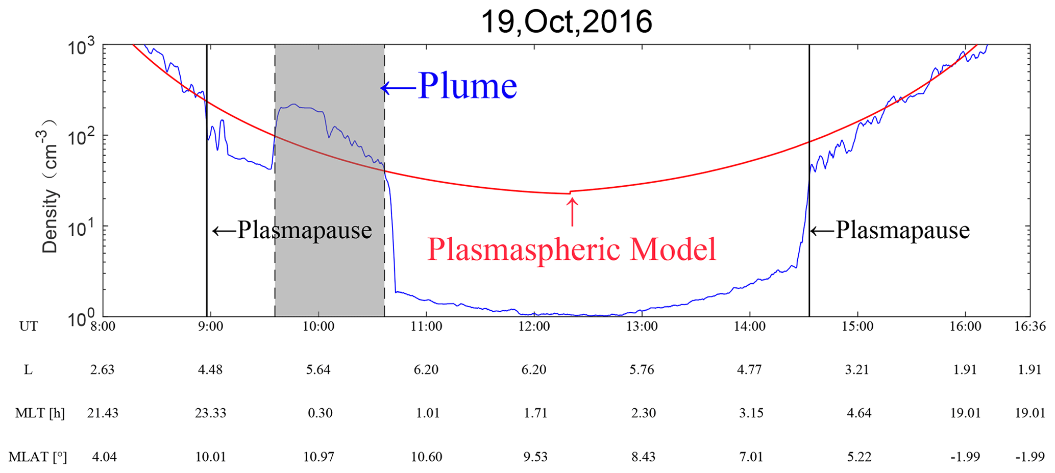
Figure 1A typical example of a plume on 19 October 2016. The blue curve represents the detected plasma density, and the red curve displays the density calculated by Sheeley et al. (2001). The position of the plasmaspause is marked by black vertical lines. The gray shadow indicates the plasmaspheric plume detected by VAP-A.
As Li et al. (2022) suggested, the number of plume events in the initial and main phases of geomagnetic storms is very small, and most plumes mainly form in the recovery phase. Partial plume events can still be observed when the geomagnetic activity recovers to quiet conditions after geomagnetic storms; this is because a relatively long time is required for the plasmasphere to recover to normal levels. Besides, referring to Halford et al. (2010) and Wang et al. (2016), the onset time of storm is defined as the time when the Dst index slope becomes negative and remains relatively negative till the minimum of the Dst index in our study. In this paper, we first focus on the relationship between the width of the plume in the interval of 10 d after the storm minimum Dst and the corresponding level of geomagnetic storm intensity (represented by the minimum Dst). According to the plume determination criteria above, we find 423 orbits with plumes (within 10 d after the minimum Dst of storm) by searching 4030 VAP-A orbits from 2013 to 2018. Since several plumes may be identified in some orbits, a total number of 586 plume events are found.
The concept of the observed plume width only has a “fuzzy” definition in the literature. To ensure the accuracy of the analysis, two judgments are adopted to represent the detected plume width. First, the width of the detected plume is defined as the Cartesian distance (ΔP) between the two ends (the entrance and exit) of the VAP-A orbit where the plume is detected:
where X0, Y0, and Z0 represent the Cartesian position of plume entry edge, and X1, Y1, and Z1 represent the Cartesian position of plume exit edge.
Second, the width is considered the difference between the magnetic local times (MLTs) of the two plume ends (ΔMLT). In this study, the corresponding geomagnetic index of the plasmaspheric plume is considered to be the minimum Dst value in the geomagnetic storm. In addition, a complication in measuring the plume width is that the plume is still rotating when VAP-A passes through the plasmasphere, which will lead to more or fewer satellite orbits in the plasmasphere. For statistical significance, the average width can reduce this influence because of the similar behavior between the entry and exit edges of the plume, and it also reminds the reader that the width measurement of the individual plume may be some error (Borovsky and Denton, 2008). To clearly reflect the statistical variation in plume width associated with geomagnetic activity, we use the averaged width of the detected plume in steps of 5 nT (Dst index) to represent the plume width in the corresponding Dst range in the study.
Figure 2 shows the widths of the 586 plumes detected above as a function of the corresponding Dst. The Cartesian distance (ΔP) and ΔMLTs are denoted by the solid black points in Fig. 2a and b, respectively. The red curves connect the averaged widths of plasmaspheric plumes in each step of the 5 nT range (plotted by red asterisks). Then, we fit the red asterisk dots through a linear function, which is drawn by a blue line. It is obvious that the blue curves are almost parallel to the Dst indices for both Fig. 2a and b. This means that the plume width is independent of the level of geomagnetic storm intensity. For Fig. 2a, the calculated Pearson correlation coefficient (marked as R), which indicates the linear relevance between the averaged Cartesian distance of plasmaspheric plumes (indicated by red asterisks) and the corresponding Dst value, is only −0.017. The P value (marked as P), which is generally adopted to express the reliability of their linear correlation, reaches 0.935. For Fig. 2b, the calculated Pearson correlation coefficient between the averaged ΔMLT of plasmaspheric plumes and the corresponding Dst value is only −0.053. The P value is 0.803. The low R and high P values in Fig. 2a and b suggest that there is almost no correlation between the widths of the above plumes and the corresponding Dst values, and their relationship may be very complicated.
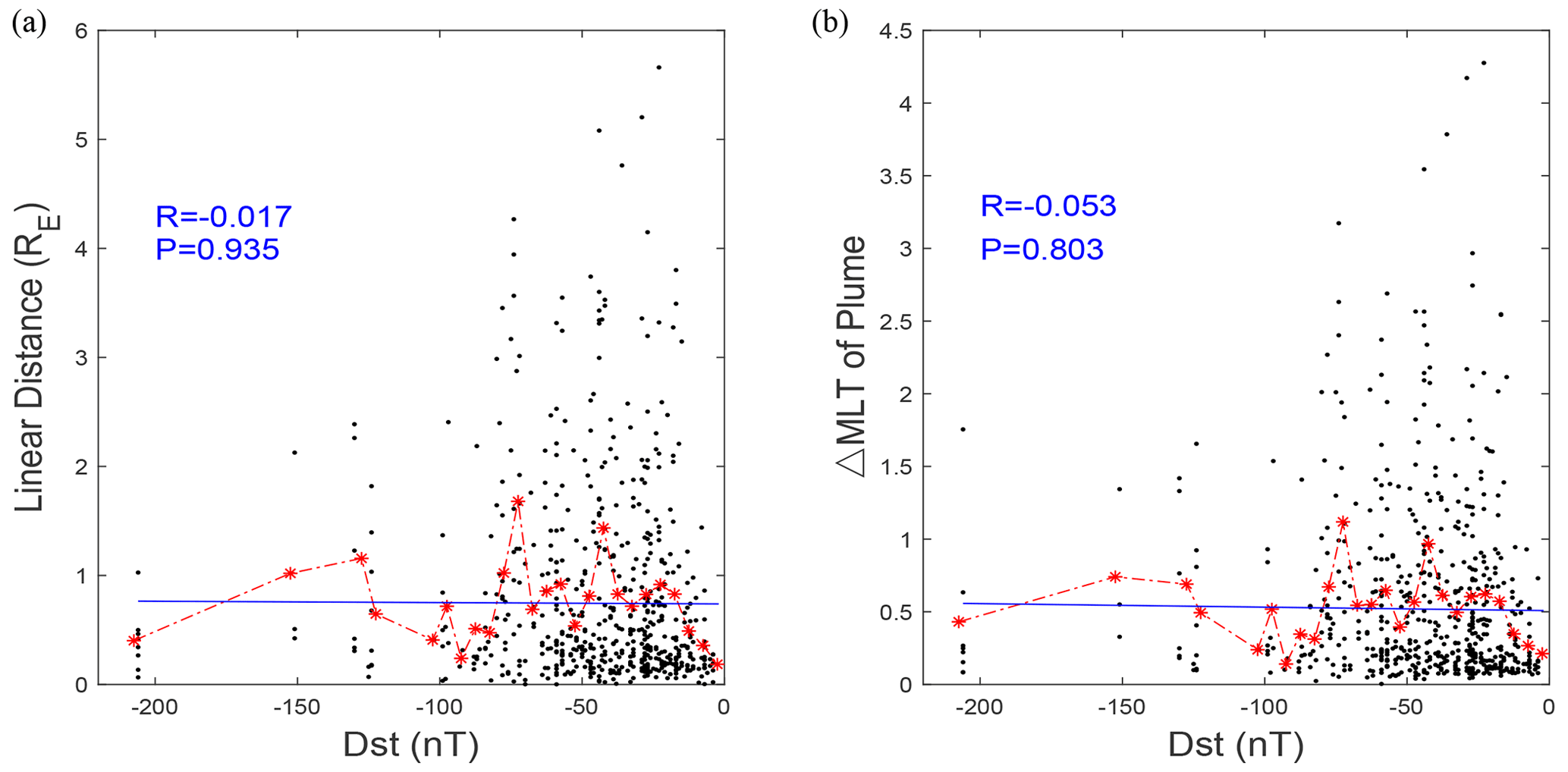
Figure 2(a) The widths of plumes as a function of Dst values are represented by solid black dots, where the width expresses the Cartesian distance between the two ends (the entrance and exit) of the VAP-A orbit where the plume is detected. The linear fitting of the plasmaspheric plume's averaged widths in each step of the 5 nT range (red asterisk points) is indicated by the blue line. (b) The format is similar to (a); however, the ΔMLT of the plasmaspheric plume is adopted to represent the width of the plume.
The formula of the Pearson correlation coefficient is as follows:
where xi and yi are two sets of data with the same number (N). As described above, we use the averaged width of the detected plume in steps of 5 nT (Dst index) to represent the plume width in the corresponding Dst range; N is equal to 15 if the geomagnetic activity levels from Dst ∼ −15 nT to Dst ∼ −90 nT are considered in the study.
An explanation of the poor relevance is that some processes may influence the structure of the plasmasphere and plume. For example, the advent of quiet conditions after geomagnetic storms can contribute to the refilling of the plasmasphere because ionospheric particles are drawn upward from low altitudes along magnetic field lines. In addition, the number of samples with geomagnetic storms that are too strong or too weak may be too few to have statistical significance. Therefore, to better understand the influence of storm intensity on the plume width, we further sifted the plume events.
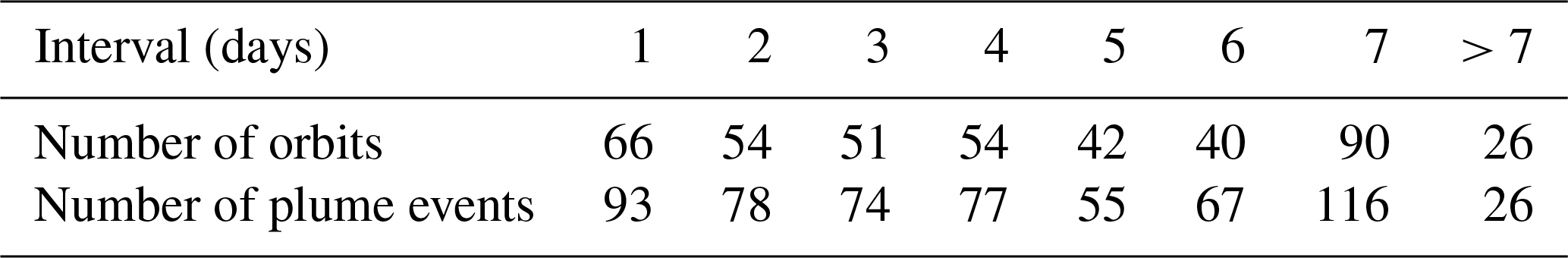
First, considering that the plasmasphere can be obviously refilled after the time of geomagnetic disturbance, we only retain the events during the recovery phase of the geomagnetic storm. This operation ensures that the main factor affecting the structure of the plume is the erosion process of the geomagnetic storm, which is the main topic in the study. Similar to the standards described in Engebretson et al. (2008), Halford et al. (2010), and Bortnik et al. (2008), we define the main phase as the period from onset of the storm until the Dst reaches its minimum value, and the end of the recovery phase is defined as the fifth day after the main phase finishes. The numbers of plume events corresponding to different time intervals (here, 1 d represents the interval of 0–24 h) after the minimum Dst are shown in Table 1. The total number of plume events in the recovery phase (the interval time is 1–5 d) is 377.
Table 1The number of events corresponding to different intervals after the minimum Dst.
Among the 377 plume events, the minimum Dst value of the most intense geomagnetic storm reaches −209 nT, but 68 % of plume events (256 events) correspond to Dst values ranging from −70 to −15 nT, and 88 % of plume events (333 events) correspond to the minimum Dst values of the most intense geomagnetic storm ranging from −90 to −15 nT. For the accuracy of statistical research, we exclude extremely intense storms in the study, and we only statistically analyze plasmaspheric plume events from −70 to −15 nT (and from −90 to −15 nT) during the recovery phase.
Moreover, in addition to the density exceeding the Sheeley model for more than 10 min outside the plasmapause, we further improve the standard of plume judgment. Referencing the method of Darrouzet et al. (2008), the ΔL of the structure (the difference in the L shell between the entrance and exit of the plume orbit) should be large enough (0.2) to be considered a plume. On the other hand, the events with excessive linear width (>3.5 RE) are also considered not plumes because they are more likely to be the cross section of the plasmasphere rather than the plume. Based on this standard, we exclude 111 plume events in the range from −70 to −15 nT and 168 plume events in the range from −90 to −15 nT.
The process of deleting events that do not match the standard is shown in Fig. 3. The solid orange dots indicate the events that are not in the recovery phase, which are beyond 5 d after the minimum Dst value. The solid purple dots indicate plume events with corresponding Dst values less than −70 nT or greater than −15 nT. The solid blue and red dots represent the tracks with ΔL less than 0.2 and Cartesian distances greater than 3.5 RE, respectively. The solid gray and black dots indicate the retained plume events with corresponding Dst ranges from −90 to −70 nT and −70 to −15 nT, respectively. Ultimately, there are 145 retained plume events in the Dst range from −70 to −15 nT, and 165 retained plume events in the Dst range from −90 to −15 nT. In addition, the spatial distribution of 586 events is shown in Fig. 4. The curves represent the VAP-A orbits while the events are observed. The colors of the curves represent the filtering process discussed above, and the corresponding event color is consistent with Fig. 3. It also shows that the retained plumes (indicated by the black curves) are mainly observed on the duskside (MLT ∼ 15:00 to ∼ 21:00).
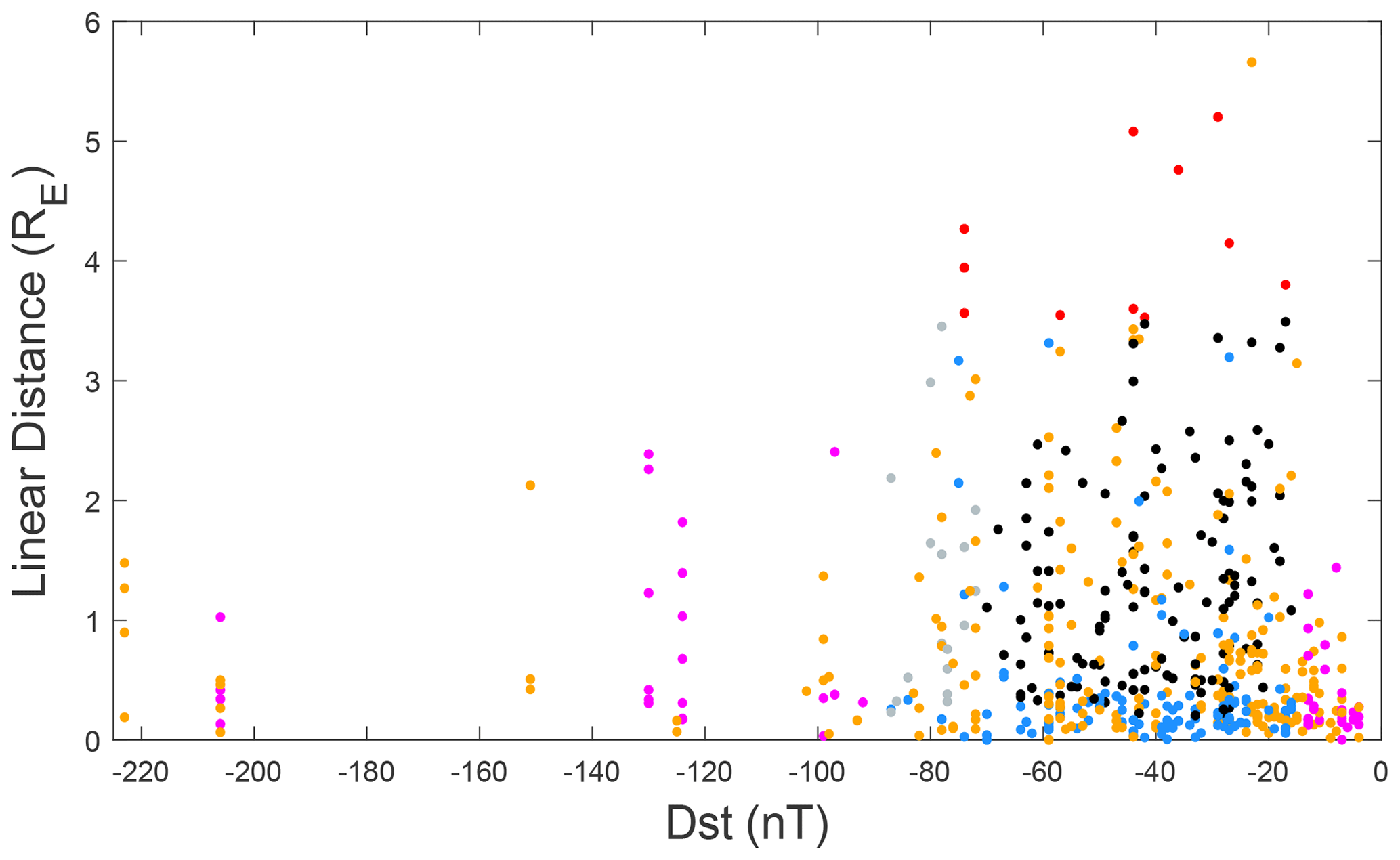
Figure 3The category of observed events: the solid orange dots indicate plume events that are not in the recovery phase. The solid purple dots display the events with a corresponding Dst index less than −70 nT or greater than −15 nT. The solid blue and red dots represent the events with ΔL less than 0.2 and Cartesian distances greater than 3.5 RE, respectively. The events in the Dst range of −70 to −15 nT and −90 to −70 nT eventually retained are indicated by black and gray dots, respectively.
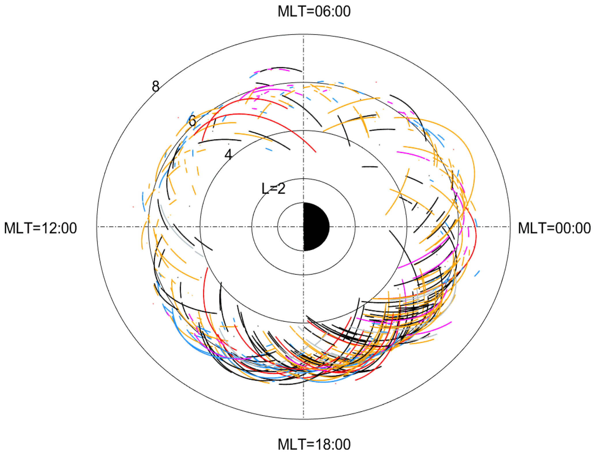
Figure 4The spatial distribution of 586 plasmaspheric plumes is shown in the MLT–L plane. The color codes are the same as those in Fig. 3.
Figure 5a and b show the correlation analysis between the retained plume width and the level of geomagnetic storm intensity with a minimum Dst of −70 to −15 nT. The formats are similar to Fig. 2a and b. Completely different from the results before the sifting plume events (as shown in Fig. 2), as indicated by the blue lines in Fig. 5, there is a considerable negative correlation between the plume width and level of corresponding geomagnetic storm intensity. This implies that as the minimum Dst value becomes lower, the width of the plasmaspheric plume tends to become narrower. As presented in Fig. 5a, the Pearson correlation coefficient between the averaged Cartesian distance of plumes and the Dst value reaches 0.619. The value of the P value is 0.042, and the low value of the P value means that it is feasible to express the relationship as a linear one. As presented in Fig. 5b, the Pearson correlation coefficient between the averaged ΔMLT and the Dst value reaches 0.546, and the P value is 0.068. The interpretations from Fig. 5a and b both imply that there is a roughly negative correlation between the width of the plume in the recovery phase and the level of geomagnetic storm intensity.
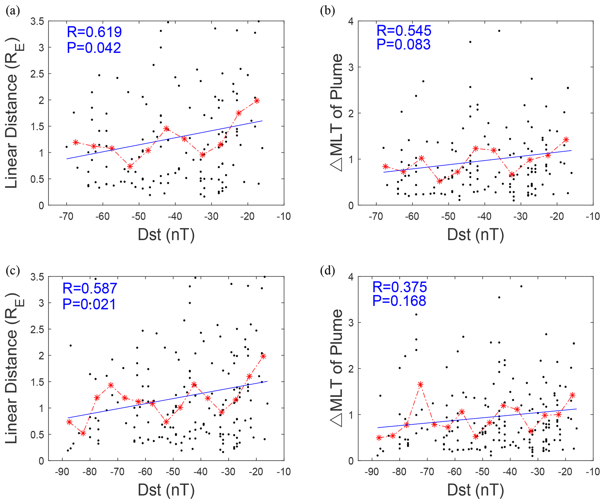
Figure 5The format is the same as in Fig. 2. However, only the retained plume events that meet more stringent sifting conditions are analyzed.
Similarly, Fig. 5c and d show the correlation analysis between the retained plume width and storm intensity with a minimum Dst from −90 to −15 nT. As exhibited in Fig. 5c, the Pearson correlation coefficient between the averaged Cartesian distance of plumes and the Dst value is 0.580. The value of the P value is 0.021. This also implies that there is a roughly negative correlation between the plume width and levels of geomagnetic storm intensity, with a minimum Dst from −90 to −15 nT. As presented in Fig. 5d, the Pearson correlation coefficient between the averaged ΔMLT and the Dst value is 0.370, and the P value is 0.170. From the perspective of the ΔMLT analysis, it seems that the negative correlation in the Dst range from −90 to −15 nT is weaker.
For the accuracy of statistical research, we exclude extremely intense storms in the study; only the plume events that correspond to intervals of minimum Dst indices from −70 to −15 and −90 to −15 nT are statistically analyzed.
It seems that the negative correlation for the events with minimum Dst from −90 to −15 nT decreases slightly compared to those with minimum Dst from −70 to −15 nT.
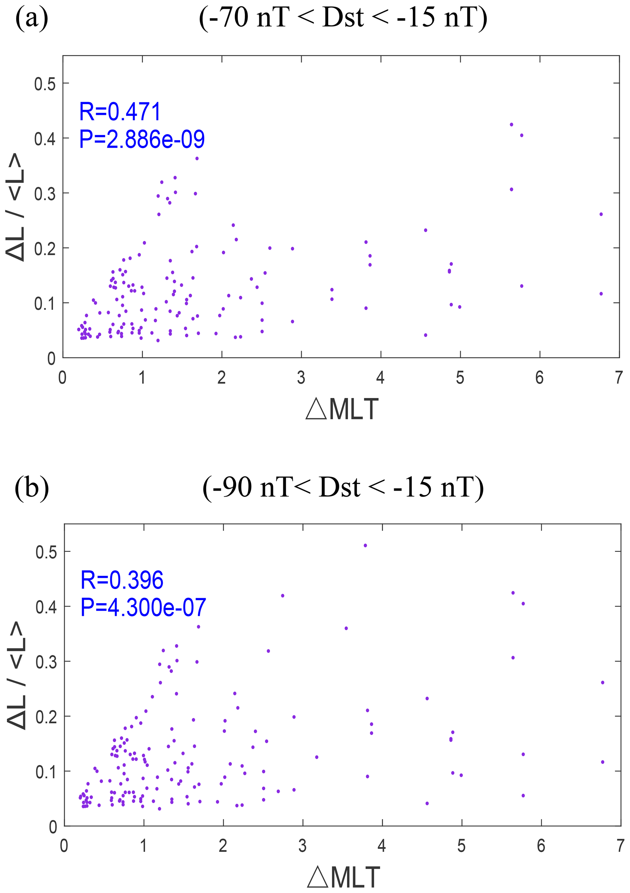
In this study, the Cartesian distance and ΔMLT are adopted to represent the detected plume width. Both methods imply that there is a negative correlation between the width of the plume in the recovery phase and the level of corresponding geomagnetic storm intensity. To compare the similarities and differences between the two standards, Fig. 6 exhibits the relationship between and the ΔMLT of plumes, where ΔL indicates the difference between the L shells of the entrance and exit of the plume detected by the VAP-A, and 〈L〉 indicates the average value of L on the plume orbit. There is a positive Pearson correlation coefficient (0.471 for the Dst range from −70 to −15 nT, 0.396 for the Dst range from −90 to −15 nT) between them, which means that when increases, the tendency of ΔMLT also enhances, although this positive correlation is not too strong. The minimal P value (∼ and ∼ , respectively) shows that the linear relationship between them is very reliability.
To clearly exhibit the effect of the storm intensity on the width of the plasmaspheric plume, the evolutions of the plumes during two geomagnetic storms (with minimum Dst values equal to −39 and −74 nT) are simulated through test particle simulations. In this study, this process differs from the plasmapause test particle (PTP) simulation which only provides the evolution of the plasmapause and plasmaspheric plume boundaries in Goldstein et al. (2004, 2014a, b); the particle simulations in this study also calculate the evolution of density in the plasmasphere and plasmaspheric plume.
3.1 Model inputs
This simulation assumes that all particles move in the dipole magnetic field model. Considering not only that the plasma motion will be driven by the combined action of the corotating electric field and convection electric field during the geomagnetic storm but also that the subauroral polarization stream (SAPS) will play a significant modification of the convection electric field, the magnetospheric electric model is assumed to consist of three parts as follows:
-
The corotation electric potential is Φrot with the following formula:
where C indicates a constant of 92, which is provided by Völk and Haerendel (1970), and r indicates the geocentric latitude.
-
The convection electric potential is expressed as follows (Maynard and Chen, 1975):
where EIM is the inner magnetospheric electric field. While the southward IMF turns southward, , and when the IMF is reverse, it is equal to 0.12⋅0.25 mV m−1. Here, the ESW is the solar wind electric field. The azimuth angle is indicated by φ, where MLT = .
-
The SAPS electric potential is an intense, radially narrow, westward flow channel that is mainly located in the dusk-to-midnight MLT area (Burke et al., 1998; Foster and Burke, 2002) and is considered to significantly modify convection. As Goldstein et al. (2005a, b, 2014b) suggest, the effects of the SAPS in the equatorial magnetosphere are driven by the Kp index, and the electric potential is described as follows:
where F(rφ), G(φ), and VS(t) are functions parameterized by the magnetic latitude, MLT(φ), time (t) and Kp index.
The detail formulas of functions are as follows:
-
The function F(rφ) treats the SAPS flow channel as a potential drop centered at radius Rs:
where Rs, α are represented in the following way:
with β=0.97 and κ=0.14; and R0 is expressed as follows:
where RE is the radius of the Earth, 6380 km.
α is expressed as
-
Based on the magnitude of the SAPS potential drop decreases eastward across the nightside, azimuthal modulation of SAPS magnitude G(φ) is set to
-
The VS(t) function describes the time regulation of SAPS:
The initial plasma density distribution is assumed to change as a function of the L shell () according to the model obtained from Sheeley et al. (2001) (the formula of the Sheeley model is expressed as Eq. 1) with no MLT dependence. In addition, for regions where the L shell is larger than 7, the electron density remains at 5 cm−3. All particles (approximately 128 000 electrons in total) emitted in the model are considered to be cold electrons and assumed to have an initial energy of 10 eV. Here, the motions of electrons are assumed to be adiabatic. We calculate the drift velocity as a combination of the velocity due to E×B drift and the bounce-averaged velocity due to gradient and curvature drifts (Roederer, 1970; Ganushkina et al., 2005; Li et al., 2021). Here, the pitch angles of the 128 000 electrons are deemed arbitrary, because the electron energy is considered to be small enough that the associated gradient-curvature drift velocity is very small (Roederer and Zhang, 2014). The motions of electrons are mainly contributed by the E×B drift. According to the simulation results, we can calculate the particle density in a certain area to reflect the evolution of the plasmasphere and plume. Notably, the actual shape of the plasmapause is too complicated to obtain its actual electron distribution function, so the above typical model electron density distribution is adopted in the research.
3.2 Evolution of plume from 19 to 20 May 2017
The geomagnetic and solar wind indices during the geomagnetic storm from 19 to 20 May 2017 are displayed in Fig. 7. As shown in Fig. 7b, at 07:02 UT, the IMF turned southward, leading to a larger negative BZ, and the geomagnetic storm began. The beginning of the geomagnetic storm is denoted by the vertical dashed blue line. The minimum Dst index of this geomagnetic storm was −39 nT. As shown in Fig. 7c, during the main phase of this geomagnetic storm (from approximately 12:00 UT on 19 May to 09:00 UT on 20 May), the maximum EIM index reached 0.4684 mV m−1. As shown in Fig. 7d, the Kp index that drove the SAPS model reached a maximum of 4+.
The test particle simulation started at 07:02 UT on 19 May 2017 (the beginning of the geomagnetic storm). The initial distribution of particle density is shown in Fig. 8a. In the contribution of the convection electric field, the particles in the plasmasphere obviously move sunward within 5 h from 07:02 to 12:02 UT on 19 May 2017 (as shown in Fig. 8b). Meanwhile, some of the plasmaspheric particles expand to high locations with L>8 and may be lost to the magnetopause boundary (Spasojevic et al., 2005). During the interval of the next 5 h, more particles move sunward and reach the model boundary (as shown in Fig. 8c), and the L shell of the plasmapause on the nightside obviously decreases. As shown in Fig. 8d and e, from 22:02 to 03:02 UT on 20 May 2017, the width of the plasmaspheric bulge gradually shrinks, and a plume gradually forms on the afternoon side. Furthermore, under the action of a corotation electric field, the plasmaspheric plume gradually shifts toward the nightside. From 08:02 to 13:02 UT on 20 May (as shown in Fig. 8f and g), as the convection electric field and SAPS electric field increase again, a large number of particles move in the sunward direction, and the plasmaspheric plume narrows with time. For most times in the recovery phase, the convection electric field becomes weaker, and the formed plasmaspheric plume slowly rotates from the afternoon side to the nightside (as shown in Fig. 8g to h). The plasma density detected by the VAP-A from 17:36 to 22:39 UT on 20 May 2017 is shown in Fig. 8i. From 18:12 to 19:53 UT on 20 May 2017, the VAP-A operated near the apogee of its orbit on the duskside, and the plume also rotated to the duskside. The orbit of the VAP-A, while it actually observed the plume, is indicated by the black curve in Fig. 8h. We can see that the observed plume roughly coincides with the simulated plume in Fig. 8h. As the positions of the simulated plume and observed plume are roughly identical at this time, we believe that the initial distribution of particles and magnetospheric electric field models used in this paper are basically reliable.
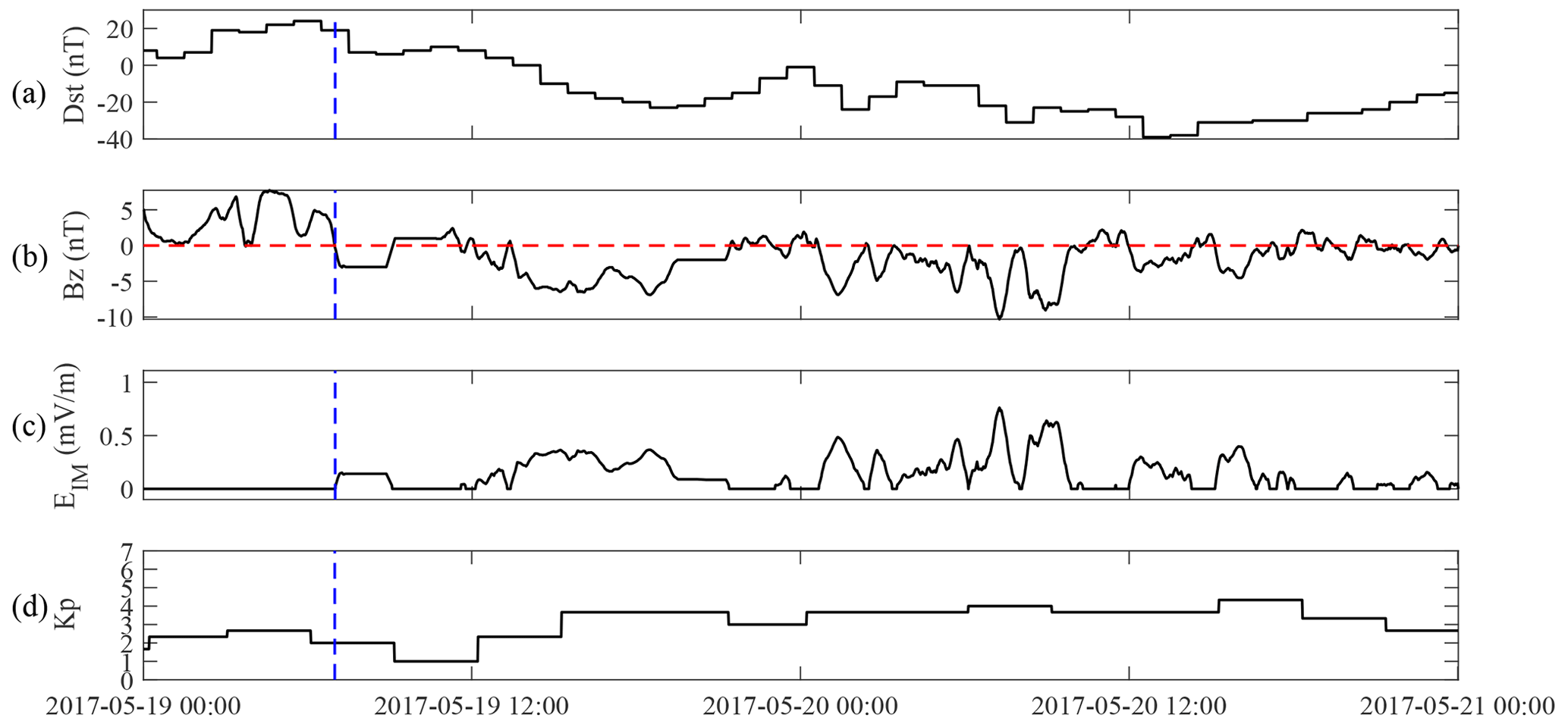
Figure 7The indices of geomagnetic activity and solar wind during the geomagnetic storm that occurred in the time interval of 19–20 May 2017: (a) Dst index, (b) BZ index in GSM coordinates. The dotted red line indicates the position where BZ is equal to 0, (c) EIM index, and (d) Kp index. The start time of the geomagnetic storm (07:02 UT on 19 May 2017) is marked by the vertical dashed blue line.
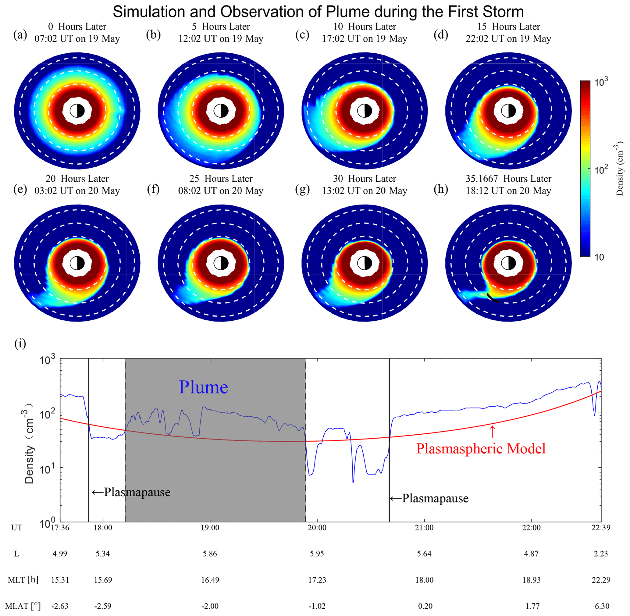
Figure 8(a–h) Equatorial plots of the plasmasphere and plume obtained by simulation in the time interval of 19–20 May 2017. The dotted white circles, from inside out, indicate L shell values of 4, 6, and 8. The simulation duration and the corresponding actual duration are represented in the title. The solid black line in (h) represents the orbit arc in which the VAP-A observed a plasmaspheric plume from 18:12 to 19:53 UT on 20 May. (i) The plasma density detected by the VAP-A from 17:36 to 22:39 UT on 20 May 2017. The gray shadow indicates the plasmaspheric plume detected by the VAP-A.
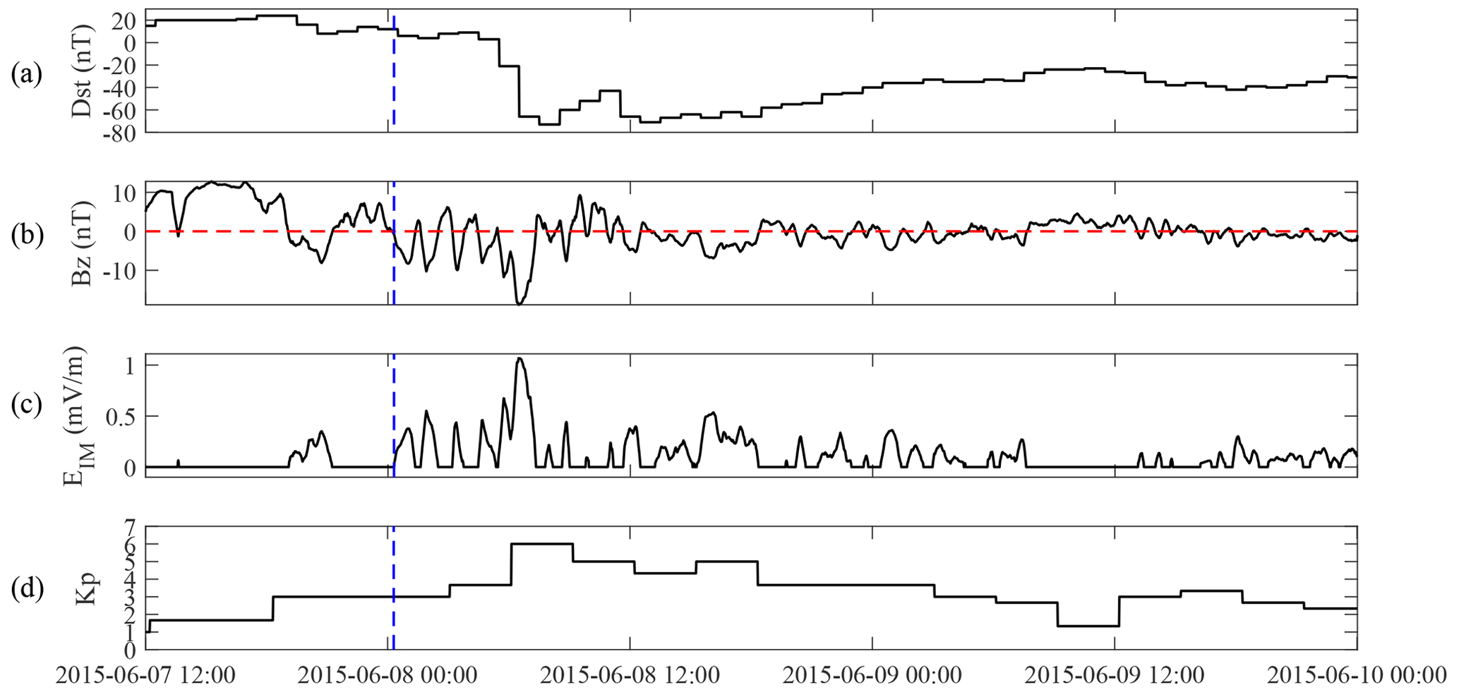
Figure 9The indices of geomagnetic activity and solar wind during the geomagnetic storm that occurred in the time interval of 8–10 June 2015; the format is the same as that in Fig. 7.
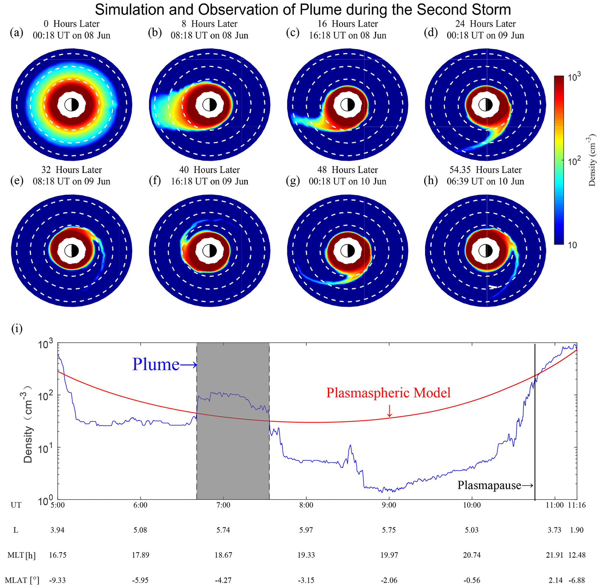
Figure 10(a–h) Equatorial plots of the plasmasphere and plume obtained by simulation in the time interval of 8–10 June 2015. The dotted white circles, from inside out, indicate L shell values of 4, 6, and 8. The simulation duration and the corresponding actual duration are represented in the title. The solid white line in (h) represents the orbit arc in which the VAP-A observed the plasmaspheric plume from 06:39 to 07:31 UT on 10 June. (i) The plasma density detected by the VAP-A from 05:00 to 11:16 UT on 10 June 2015. The gray shadow indicates the plasmaspheric plume detected by the VAP-A.
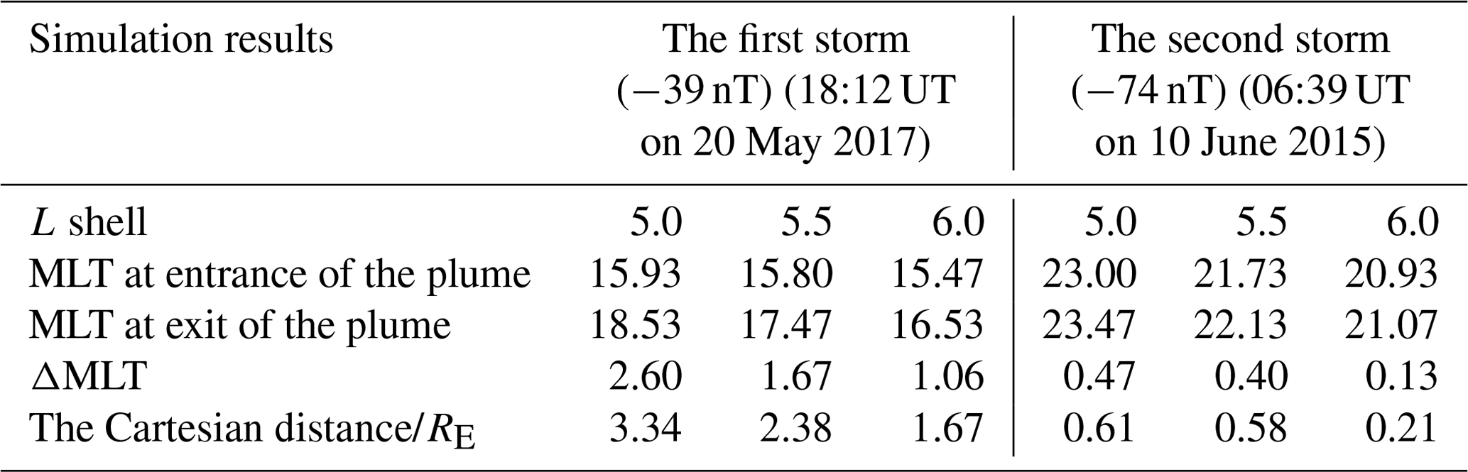
Table 2The widths of the simulated plume at different L shells during the above two geomagnetic storms.
3.3 Evolution of plume from 8–10 June 2015
The geomagnetic and solar wind indices during the geomagnetic storm from 8 to 10 June 2015 are shown in Fig. 9. The geomagnetic storm began at 00:18 UT on 8 June 2015 (denoted by the blue line). As shown in Fig. 9a, the minimum Dst index of this geomagnetic storm was −74 nT, which was much lower than that during the storm presented in Sect. 3.2. At the beginning of the geomagnetic storm, the BZ turned southward, and the EIM value (calculated from ESW) became a relatively large positive value. The maximum EIM in this geomagnetic storm was 1.0674 mV m−1, which was much greater than the 0.4684 mV m−1 obtained from the geomagnetic storm presented in Sect. 3.2. Meanwhile, the maximum Kp index reached 6 in the main phase. It was also much larger than 4+ presented in the last storm. Larger EIM and Kp indices both implied that convection during this geomagnetic storm was much more intense than that during the geomagnetic storm from 19 to 20 May 2017.
Figure 10a shows the electron density distribution during the first minute of the simulation during this geomagnetic storm. Then, under the contribution of a continuous convection electric field, the plasma in the outer part of the plasmasphere moves along the E×B-drift paths from 00:19 UT on 8 June to 06:39 UT on 10 June. As shown in Fig. 10b and c, the more intense convection electric field brings about a larger number of particles on the dayside moving sunward and extending out of the model boundary, and the particles on the nightside in the plasmasphere move faster toward the Earth. As shown in Fig. 10d, the particles in the outer part of the plasmasphere dissipate at 00:18 UT on 9 June, and a narrower plume emerges near the duskside. During the recovery phase of the geomagnetic storm, as shown from Fig. 10e to h, the formed narrow plume revolves around the Earth. Finally, the VAP-A observes the structure of the plume from 06:39 to 07:31 UT on 10 June 2015 (as shown in Fig. 10i), and the orbit of the probe during this time interval is indicated in Fig. 10h. The observations and simulations both suggest that the L shell of the plasmapause is lower than that presented in Sect. 3.2. Although there is some difference in the MLT between the simulated plume and observed plume (approximately 1 MLT, which may be due to a simulation time that is too long), the results imply that the width of the plume is much narrower than that during the geomagnetic storm from 19 to 20 May 2017.
3.4 Comparison of simulation results
To better exhibit the difference in the simulated plume width during the above two geomagnetic storms, we calculated the Cartesian distances and ΔMLTs at positions where the L shell was equal to 5, 5.5, and 6. The calculated results are shown in Table 2. As presented in Table 2, at the same L shell, regardless of Cartesian distances and ΔMLT, the simulated plume driven by stronger geomagnetic storms is always narrower.
In this study, we present statistical research on the relationship between the widths of plumes and the intensities of geomagnetic storms by analyzing the data collected by the VAP-A. Here, the widths of the detected plume are defined as the Cartesian distance and ΔMLT of the detected plume orbit. In the first step, by directly analyzing all 586 potential plume events after the minimum Dst of a geomagnetic storm, we find that there is almost no correlation between plume width and the level of storm intensity. This result is similar to the conclusion obtained from Borovsky and Denton (2008), which suggests that the linear correlation coefficient between them is almost 0. Since the plasmasphere can be eroded by the enhanced convection electric field during geomagnetic storms (Krall et al., 2017), the enhanced convection field causes low energy plasma drainage to the magnetopause (Denton et al., 2005). We consider that the level of storm intensity may affect the width of the plume in some conditions. In the second step, we define the end of the recovery phase as 5 d after the main phase finishes. Only the plumes in the recovery phase interval are analyzed. Moreover, the criterion of plumes for statistical investigation is further improved. This result suggests that there is a negative correlation between the plume width and absolute value of the minimum Dst value during the storm, although the negative correlation is not very strong.
To explain the negative correlation between them during the recovery phase of the geomagnetic storm, the group test particle simulation is adopted to reveal the dynamic evolutions of the plasmasphere and plume during two geomagnetic storms (with minimum Dst values of −39 and −74 nT, respectively). By comparing the evolutions during the two storms, we find that in the more intense geomagnetic storm, the erosion of the plasmasphere is more severe, most particles in the outer part of the plasmasphere are dissipated during the initial and main phases, and a narrower plume is exhibited during the recovery phase. Although the evolutions of plasmaspheres and plumes may be very complicated, the above simulation results provide a reasonable candidate explanation for the negative correlation between level of geomagnetic storm intensity and plume width during the recovery phase of geomagnetic storms.
As shown in Fig. 4, most plume events are mainly observed on the duskside; the relationship between the plume width and its MLT is also a meaningful work, which will be studied in our next project. Since there may be a short time delay with several minutes between the changes of ESW and EIM (Nishimura et al., 2009), a more precise and real-time EIM model will be discussed and explored in the future. This paper analyzes the plume events with Dst values ranging from −90 to −15 nT during the recovery phase. In the future study, we will use other geomagnetic activity indices to analyze the relationship between plume width and magnetic storm intensity, such as Kp, and AE, thus studying the correlation between the plume width and substorm activity.
The data of EMFISIS aboard the Van Allen Probes are publicly available at the EMFISIS website (http://emfisis.physics.uiowa.edu/data/index, Kletzing et al., 2013). The OMNI data are provided at the SPDF website (http://cdaweb.gsfc.nasa.gov, NASA, 2022).
The conceptional idea of this study was developed by HL and ZYa. HL and ZYa wrote the paper, and ZYa revised it. ZO and XD helped substantially with the analysis. ZYu and ZO contributed to the Van Allen Probe data processing. All authors discussed the results.
The contact author has declared that none of the authors has any competing interests.
Publisher's note: Copernicus Publications remains neutral with regard to jurisdictional claims in published maps and institutional affiliations.
The data of EMFISIS aboard the Van Allen Probes are from (http://emfisis.physics.uiowa.edu/data/index. The Dst and KP data are provided by OMNI at http://cdaweb.gsfc.nasa.gov.
This research has been supported by the National Natural Science Foundation of China (grant no. 42064009).
This paper was edited by Elias Roussos and reviewed by three anonymous referees.
Borovsky, J. E. and Denton, M. H.: A statistical look at plasmaspheric drainage plumes, J. Geophys. Res., 113, A09221, https://doi.org/10.1029/2007JA012994, 2008.
Bortnik, J., Cutler, J. W., Dunson, C., Bleier, T. E., and McPherron, R. L.: Characteristics of low-latitude Pc1 pulsations during geomagnetic storms, J. Geophys. Res., 113, A04201, https://doi.org/10.1029/2007JA012867, 2008.
Burke, W. J., Maynard, N. C., Hagan, M. P., Wolf, R. A., Wilson, G. R., Gentile, L. C., Gussenhoven, M. S., Huang, C. Y., Garner, T. W., and Rich, F. J.: Electrodynamics of the inner magnetosphere observed in the dusk sector by CRRES and DMSP during the magnetic storm of June 4–6, 1991, J. Geophys. Res., 103, 29399–29418, https://doi.org/10.1029/98JA02197, 1998.
Chen, A. J. and Grebowsky, J. M.: Plasma tail interpretations of pronounced detached plasma regions measured by Ogo 5, J. Geophys. Res., 79, 3851–3855, https://doi.org/10.1029/JA079i025p03851, 1974.
Darrouzet, F., De Keyser, J., Décréau, P. M. E., El Lemdani-Mazouz, F., and Vallières, X.: Statistical analysis of plasmaspheric plumes with Cluster/WHISPER observations, Ann. Geophys., 26, 2403–2417, https://doi.org/10.5194/angeo-26-2403-2008, 2008.
Denton, M. H., Thomsen, M. F., Korth, H., Lynch, S., Zhang, J. C., and Liemohn, M. W.: Bulk plasma properties at geosynchronous orbit, J. Geophys. Res., 110, A07223, https://doi.org/10.1029/2004JA010861, 2005.
Dungey, J. W.: Interplanetary Magnetic Field and the Auroral Zones, Phys. Rev. Lett., 6, 47–48, https://doi.org/10.1103/PhysRevLett.6.47, 1961.
Engebretson, M. J., Lessard, M. R., Bortnik, J., Green, J. C., Horne, R. B., Detrick, D. L., Weatherwax, A. T., Manninen, J., Petit, N. J., Posch, J. L., and Rose, M. C.: Pc1–Pc2 waves and energetic particle precipitation during and after magnetic storms: Superposed epoch analysis and case studies, J. Geophys. Res., 113, A01211, https://doi.org/10.1029/2007JA012362, 2008.
Foster, J. C. and Burke, W. J.: SAPS: A new categorization for sub-auroral electric fields, EOS T. Am. Geophys. Un., 83, 393–394, https://doi.org/10.1029/2002EO000289, 2002.
Ganushkina, N. Yu., Pulkkinen, T. I., and Fritz, T.: Role of substorm-associated impulsive electric fields in the ring current development during storms, Ann. Geophys., 23, 579–591, https://doi.org/10.5194/angeo-23-579-2005, 2005.
Goldstein, J., Sandel, B. R., Thomsen, M. F., Spasojević, M., and Reiff, P. H.: Simultaneous remote sensing and in situ observations of plasmaspheric drainage plumes, J. Geophys. Res., 109, A03202, https://doi.org/10.1029/2003JA010281, 2004.
Goldstein, J., Burch, J. L., and Sandel, B. R.: Magnetospheric model of subauroral polarization stream, J. Geophys. Res., 110, A09222, https://doi.org/10.1029/2005JA011135, 2005a.
Goldstein, J., Kanekal, S., Baker, D. N., and Sandel, B. R.: Dynamic relationship between the outer radiation belt and the plasmapause during March–May 2001, Geophys. Res. Lett., 32, L15104, https://doi.org/10.1029/2005GL023431, 2005b.
Goldstein, J., De Pascuale, S., Kletzing, C., Kurth, W., Genestreti, K. J., Skoug, R. M., Larsen, B. A., Kistler, L. M., Mouikis, C., and Spence, H.: Simulation of Van Allen Probes plasmapause encounters, J. Geophys. Res.-Space, 119, 7464–7484, https://doi.org/10.1002/2014JA020252, 2014a.
Goldstein, J., Thomsen, M. F., and DeJong, A.: In situ signatures of residual plasmaspheric plumes: Observations and simulation, J. Geophys. Res.-Space, 119, 4706–4722, https://doi.org/10.1002/2014JA019953, 2014b.
Grebowsky, J. M.: Model study of plasmapause motion, J. Geophys. Res., 75, 4329–4333, https://doi.org/10.1029/JA075i022p04329, 1970.
Grison, B., Hanzelka, M., Breuillard, H., Darrouzet, F., Santolík, O., Cornilleau-Wehrlin, N., and Dandouras, I.: Plasmaspheric plumes and EMIC rising tone emissions, J. Geophys. Res.-Space, 123, 9443–9452, https://doi.org/10.1029/2018JA025796, 2018.
Halford, A. J., Fraser, B. J., and Morley, S. K.: EMIC wave activity during geomagnetic storm and nonstorm periods: CRRES results, J. Geophys. Res., 115, A12248, https://doi.org/10.1029/2010JA015716, 2010.
Kim, K.-C. and Shprits, Y.: Statistical analysis of hiss waves in plasmaspheric plumes using Van Allen Probe observations, J. Geophys. Res.-Space, 124, 1904–1915, https://doi.org/10.1029/2018JA026458, 2019.
Kletzing, C. A., Kurth, W. S., Acuna, M., MacDowall, R. J., Torbert, R. B., Averkamp, T., Bodet, D., Bounds, S. R., Chutter, M., Connerney, J., Crawford, D., Dolan, J. S., Dvorsky, R., Hospodarsky, G. B., Howard, J., Jordanova, V., Johnson, R. A., Kirchner, D. L., Mokrzycki, B., Needell, G., Odom, J., Mark, D., Pfaff, R., Phillips, J. R., Piker, C. W., Remington, S. L., Rowland, D., Santolik, O., Schnurr, R., Sheppard, D., Smith, C. W., Thorne, R. M., and Tyler, J.: The Electric and Magnetic Field Instrument Suite and Integrated Science (EMFISIS) on RBSP, Space Sci. Rev., 179, 127–181, https://doi.org/10.1007/s11214-013-9993-6, 2013 (data available at: http://emfisis.physics.uiowa.edu/data/index, last access: 10 January 2022).
Krall, J., Huba, J. D., and Sazykin, S.: Erosion of the plasmasphere during a storm, J. Geophys. Res.-Space, 122, 9320–9328, https://doi.org/10.1002/2017JA024450, 2017.
Kurth, W. S., De Pascuale, S., Faden, J. B., Kletzing, C. A., Hospodarsky, G. B., Thaller, S., and Wygant, J. R.: Electron densities inferred from plasma wave spectra obtained by the Waves instrument on Van Allen Probes, J. Geophys. Res.-Space, 120, 904–914, https://doi.org/10.1002/2014JA020857, 2015.
Lakhina, G. S., Tsurutani, B. T., Kojima, H., and Matsumoto, H.: “Broadband” plasma waves in the boundary layers, J. Geophys. Res., 105, 27791–27831, https://doi.org/10.1029/2000JA900054, 2000.
Li, H., Li, W., Ma, Q., Nishimura, Y., Yuan, Z., Boyd, A. J., Shen, X., Tang, R., and Deng, X.: Attenuation of plasmaspheric hiss associated with the enhanced magnetospheric electric field, Ann. Geophys., 39, 461–470, https://doi.org/10.5194/angeo-39-461-2021, 2021.
Li, H., Fu, T., Tang, R., Yuan, Z., Yang, Z., Ouyang, Z., and Deng, X.: Statistical study and corresponding evolution of plasmaspheric plumes under different levels of geomagnetic storms, Ann. Geophys., 40, 167–177, https://doi.org/10.5194/angeo-40-167-2022, 2022.
Ma, Q., Li, W., Zhang, X.-J., Bortnik, J., Shen, X.-C., Connor, H. K., Boyd, A. J., Kurth, W. S., Hospodarsky, G. B., Claudepierre, S. G., Reeves, G. D., and Spence, H. E.: Global survey of electron precipitation due to hiss waves in the Earth's plasmasphere and plumes, J. Geophys. Res., 126, e2021JA029644, https://doi.org/10.1029/2021JA029644, 2021.
Mauk, B. H., Fox, N. J., Kanekal, S. G., Kessel, R. L., Sibeck, D. G., and Ukhorskiy, A.: Science Objectives and Rationale for the Radiation Belt Storm Probes Mission, in: The Van Allen Probes Mission, edited by: Fox, N. and Burch, J. L., Springer, Boston, MA, https://doi.org/10.1007/978-1-4899-7433-4_2, 2012.
Maynard, N. C. and Chen, A. J.: Isolated cold plasma regions: Observations and their relation to possible production mechanisms, J. Geophys. Res., 80, 1009–1013, https://doi.org/10.1029/JA080i007p01009, 1975.
Moldwin, M. B., Downward, L., Rassoul, H. K., Amin, R., and Anderson, R. R.: A new model of the location of the plasmapause: CRRES results, J. Geophys. Res., 107, 1339, https://doi.org/10.1029/2001JA009211, 2002.
Moldwin, M. B., Howard, J., Sanny, J., Bocchicchio, J. D., Rassoul, H. K., and Anderson, R. R.: Plasmaspheric plumes: CRRES observations of enhanced density beyond the plasmapause, J. Geophys. Res., 109, A05202, https://doi.org/10.1029/2003JA010320, 2004.
NASA: OMNI data, NASA [data set], http://cdaweb.gsfc.nasa.gov, last access: 10 January 2022.
Nishimura, Y., Kikuchi, T., Wygant, J., Shinbori, A., Ono, T., Matsuoka, A., Nagatsuma, T., and Brautigam, D.: Response of convection electric fields in the magnetosphere to IMF orientation change, J. Geophys. Res., 114, A09206, https://doi.org/10.1029/2009JA014277, 2009.
Roederer, J. G.: Periodic Drift Motion and Conservation of the Third Adiabatic Invariant, in: Dynamics of Geomagnetically Trapped Radiation, Physics and Chemistry in Space, Vol. 2, Springer, Berlin, Heidelberg, https://doi.org/10.1007/978-3-642-49300-3_3, 1970.
Roederer, J. G., and Zhang, H.: Dynamics of Magnetically Trapped Particles, 2nd Edn., Springer, New York, https://doi.org/10.1007/978-3-642-41530-2, 2014.
Sheeley, B. W., Moldwin, M. B., Rassoul, H. K., and Anderson, R. R.: An empirical plasmasphere and trough density model: CRRES observations, J. Geophys. Res., 106, 25631–25641, https://doi.org/10.1029/2000JA000286, 2001.
Spasojevic, M. and Inan, U. S.: Drivers of chorus in the outer dayside magnetosphere, J. Geophys. Res., 115, A00F09, https://doi.org/10.1029/2009JA014452, 2010.
Spasojevic, M., Thomsen, M. F., Chi, P. J., and Sandel, B. R.: Afternoon Subauroral Proton Precipitation Resulting from Ring Current – Plasmasphere Interaction, AGU Fall Meeting Abstracts, 159, 85–99, https://doi.org/10.1029/159gm06, 2005.
Su, Z., Liu, N., Zheng, H., Wang, Y., and Wang, S.: Large-amplitude extremely low frequency hiss waves in plasmaspheric plumes, Geophys. Res. Lett., 45, 565–577, https://doi.org/10.1002/2017GL076754, 2018.
Usanova, M. E., Darrouzet, F., Mann, I. R., and Bortnik, J.: Statistical analysis of EMIC waves in plasmaspheric plumes from Cluster observations, J. Geophys. Res.-Space, 118, 4946–4951, https://doi.org/10.1002/jgra.50464, 2013.
Völk, H. and Haerendel, G.: Magnetospheric Electric Fields, in: Intercorrelated Satellite Observations Related to Solar Events, edited by: Manno, V. and Page, D. E., Astrophysics and Space Science Library, Vol. 19, Springer, Dordrecht, https://doi.org/10.1007/978-94-010-3278-0_19, 1970.
Wang, D., Yuan, Z., Yu, X., Huang, S., Deng, X., Zhou, M., and Li, H.: Geomagnetic storms and EMIC waves: Van Allen Probe observations, J. Geophys. Res.-Space, 121, 6444–6457, https://doi.org/10.1002/2015JA022318, 2016.
Yu, X., Yuan, Z., Wang, D., Huang, S., Qiao, Z., Yu, T., and Yao, F.: Excitation of oblique O+ band EMIC waves in the inner magnetosphere driven by hot H+ with ring velocity distributions, J. Geophys. Res.-Space, 121, 11101–11112, https://doi.org/10.1002/2016JA023221, 2016.
Yuan, Z., Deng, X., Lin, X., Pang, Y., Zhou, M., Décréau, P. M. E., Trotignon, J. G., Lucek, E., Frey, H. U., and Wang, J.: Link between EMIC waves in a plasmaspheric plume and a detached sub-auroral proton arc with observations of Cluster and IMAGE satellites, Geophys. Res. Lett., 37, L07108, https://doi.org/10.1029/2010GL042711, 2010.
Zhang, W., Ni, B., Huang, H., Summers, D., Fu, S., Xiang, Z., Gu, X., Cao, X., Lou, L., and Hua, M.: Statistical properties of hiss in plasmaspheric plumes and associated scattering losses of radiation belt electrons, Geophys. Res. Lett., 46, 5670–5680, https://doi.org/10.1029/2018GL081863, 2019.