Reconstruction of precipitating electrons and three-dimensional structure of a pulsating auroral patch from monochromatic auroral images obtained from multiple observation points

In recent years, aurora observation networks using high-sensitivity cameras have been developed in the polar regions. These networks allow dimmer auroras, such as pulsating auroras (PsAs), to be observed with a high signal-to-noise ratio. We reconstructed the horizontal distribution of precipitating electrons using computed tomography with monochromatic PsA images obtained from three observation points. The three-dimensional distribution of the volume emission rate (VER) of the PsA was also reconstructed. The characteristic energy of the reconstructed precipitating electron flux ranged from 6 to 23 keV, and the peak altitude of the reconstructed VER ranged from 90 to 104 km. We evaluated the results using a model aurora and compared the model's electron density with the observed one. The electron density was reconstructed correctly to some extent, even after a decrease in PsA intensity. These results suggest that the horizontal distribution of precipitating electrons associated with PsAs can be effectively reconstructed from ground-based optical observations.

1 Introduction

Aurora computed tomography (ACT) is a method for reconstructing the three-dimensional (3-D) volume emission rate (VER) of auroral emission based on monochromatic auroral images obtained from multiple observation points (e.g., Aso et al., 1990). The horizontal distribution of precipitating electron flux can be simultaneously obtained using ACT without rocket or satellite observations (Tanaka et al., 2011). Previous studies have applied ACT to bright and well-shaped discrete auroras, such as the quiet arc during the substorm growth phase and multiple auroral arcs (Aso et al., 1990, 1993, 1998; Frey et al., 1996; Nygrén et al., 1997; Tanaka et al., 2011). However, ACT has not been applied to pulsating auroras (PsAs).

A PsA is a type of diffuse aurora that appears as irregular patches showing quasi-periodic on–off switching of its intensity with a periodicity of ∼ 2–20 s (Yamamoto, 1988). The intensity is somewhat dimmer than that of a typical discrete aurora (some hundreds of rayleighs (R) up to tens of kilorayleighs at 557.7 nm; a few hundred rayleighs to ∼ 10 kR at 427.8 nm) (McEwen et al., 1981). It has been difficult to apply ACT to PsAs because the signal-to-noise ratio (SNR) of PsA images is lower than those of discrete aurora images. However, remote operation of many high-sensitivity cameras via the internet and an archive system capable of storing a massive amount of aurora data make it possible to observe PsAs with a high SNR.

The Magnetometers Ionospheric Radars All-sky Cameras Large Experiment (MIRACLE) network consists of nine all-sky cameras (ASCs) located in the Fennoscandian region. Two of the ASCs with intensified charge-coupled devices (ICCDs) were replaced with cameras possessing newer electron-multiplying CCD (EMCCD) technology in 2007 (Sangalli et al., 2011). Ogawa et al. (2020a) developed a low-cost multiwavelength imaging system for aurora and airglow studies and installed Watec monochromatic imagers (WMIs) at several locations in the north and south polar regions. A WMI consists of a highly sensitive CCD camera made by Watec Co., Ltd (Japan). These cameras are suitable for studying very faint auroral structures such as PsAs. In this study, we attempted to use these high-sensitivity cameras and ACT methods to reconstruct the 3-D VER of a PsA patch and the horizontal distribution of precipitating electrons for the first time.

2 Data and methods

MIRACLE ASCs observed PsA patches from Kilpisjärvi (KIL; 69.05^∘ N, 20.36^∘ E), Abisko (ABK; 68.36^∘ N, 18.82^∘ E), and WMI ASCs at Skibotn (SKB; 69.35^∘ N, 18.82^∘ E) during the substorm recovery phase from 00:00 to 02:00 UT on 18 February 2018. These ASCs have a common field of view, as shown in Fig. 1b. The position of Tromsø (TRO; 69.58^∘ N, 19.23^∘ E), where the European Incoherent Scatter Scientific Association (EISCAT) radar operates, is also shown. We selected 427.8 nm auroral images in which PsA patches were detected at the EISCAT radar observation point. The reconstructed results were compared with the electron density observed using the EISCAT radar in Sect. 3.4. Figure 1a shows 427.8 nm auroral images obtained by the three ASCs from 00:53:30 to 00:53:42 UT. The temporal resolution of each ASCs was 2 s. A median filter of 3 × 3 pixels was applied to auroral images to improve the SNR. We also composited auroral images obtained from four WMI CCD cameras of the same type at SKB. The auroral images at SKB were calibrated to derive the absolute emission intensity using the optical facilities at the National Institute of Polar Research, Japan (Ogawa et al., 2020b), and have a time ambiguity of ∼ 1–2 s. We determined the time when the auroral image was obtained by aligning the temporal changes in the PsA patch, as shown in auroral images from ABK, KIL, and SKB. The ACT method used in this study is based on the method proposed by Tanaka et al. (2011). We adopted an oblique coordinate system with the origin (O) at coordinates of 69.4^∘ N, 19.2^∘ E. The x axis was antiparallel to the horizontal component of the geomagnetic field, the y axis was eastward, and the z axis was antiparallel to the geomagnetic field and perpendicular to the y axis (see Fig. 2 in Tanaka et al., 2011). The simulation region ranged from −75 to 75 km, from −100 to 100 km, and from 80 to 180 km for the x, y, and z axes, respectively. We set the energy (E) range to extend from 300 eV to 100 keV. The energy axis contains the information on the auroral emission altitude. This is because the higher the electron energy, the lower the stopping height of the precipitating electrons. This reconstruction region was divided linearly into n_x × n_y × n_z voxels along the x, y, and z axes and logarithmically into n_E bins in the E direction. We set the parameters n_x, n_y, n_z, and n_E to 75, 100, 50, and 50, respectively, corresponding to a spatial mesh size of 2 × 2 × 2 km. These parameters were selected so that each voxel has at least one line-of-sight crossing from the pixels in the auroral images.

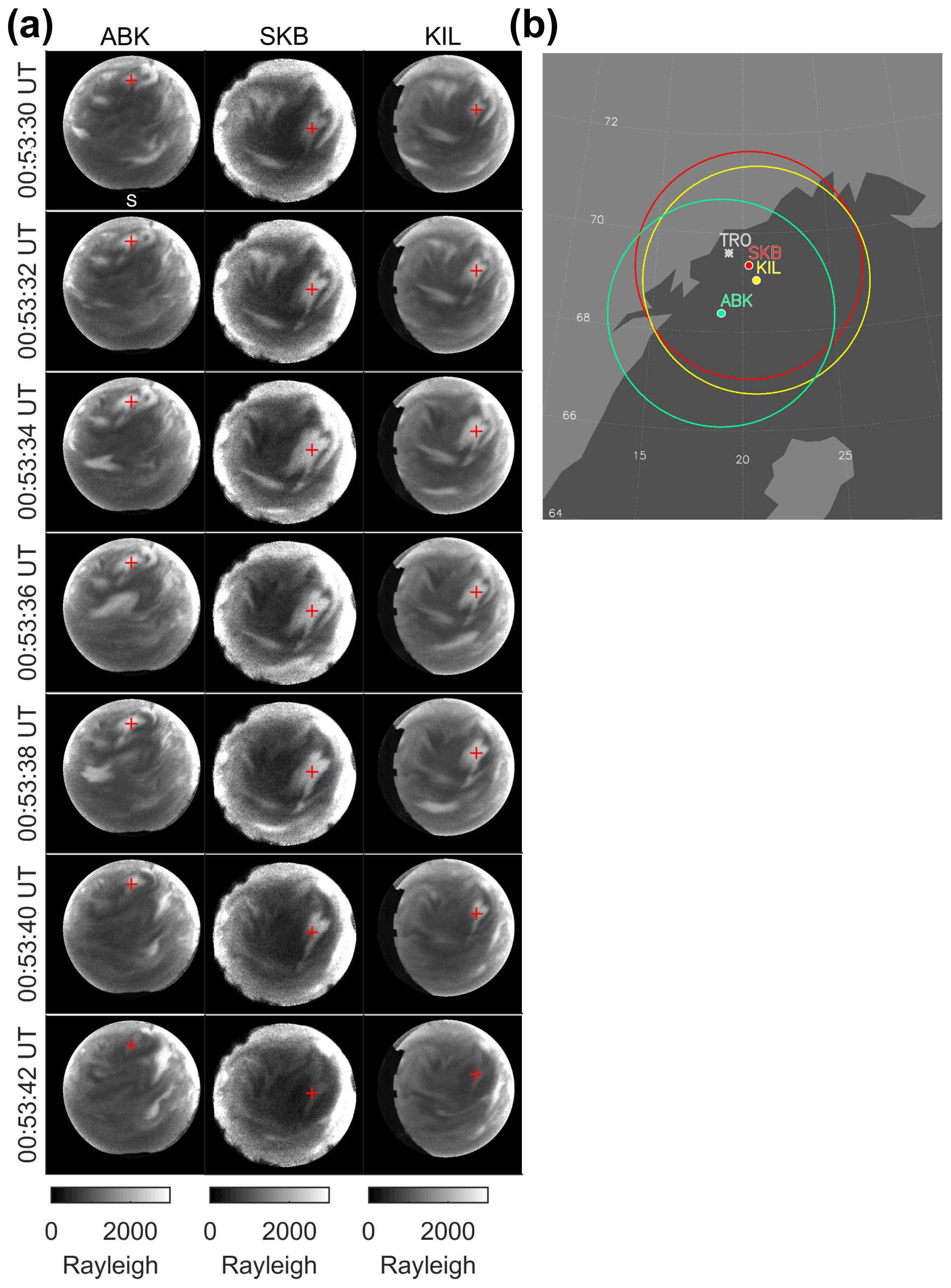
Figure 1 (a) Successive auroral images from Abisko (ABK), Skibotn (SKB), and Kilpisjärvi (KIL) from 00:53:30 to 00:53:42 UT on 18 February 2018. (b) Locations and fields of view of all-sky cameras at ABK (green), SKB (red), and KIL (yellow) at an altitude of 100 km. The location of Tromsø (TRO) is shown by a gray asterisk.

The differential flux of precipitating electrons was reconstructed by maximizing the posterior probability $P\left(\mathit{f}|\stackrel{\mathrm{̃}}{\mathit{g}}\right)$, where f is a vector of the differential flux of precipitating electrons, and $\stackrel{\mathrm{̃}}{\mathit{g}}$ is a vector of gray levels at pixels in the auroral images obtained with ASCs. According to Bayes' theorem, the posterior probability $P\left(\mathit{f}|\stackrel{\mathrm{̃}}{\mathit{g}}\right)$ is given by (Tanaka et al., 2011)

$$\begin{array}{}\text{(1)}& \begin{array}{rl}P\left(\mathit{f}|\stackrel{\mathrm{̃}}{\mathit{g}}\right)& \propto \exp [-{\displaystyle \frac{\mathrm{1}}{\mathrm{2}}}\mathit{\{}{\left(\stackrel{\mathrm{̃}}{\mathit{g}}-\mathit{g}\left(\mathit{f}\right)\right)}^T{\mathbf{\Sigma }}^{-\mathrm{1}}\left(\stackrel{\mathrm{̃}}{\mathit{g}}-\mathit{g}\left(\mathit{f}\right)\right)\\ & +{\displaystyle \frac{{∥{\mathrm{\nabla }}^{\mathrm{2}}\mathit{f}∥}^{\mathrm{2}}}{{\mathit{\sigma }}^{\mathrm{2}}}}\mathit{\left\}}\right],\end{array}\end{array}$$

where g(f) is a vector of gray levels obtained by line-integrating the VER in the line-of-sight direction from each pixel (Eq. 8 in Tanaka et al., 2011). The VER was derived from model f using the aurora emission model (Eq. 3 in Tanaka et al., 2011). Σ⁻¹ is the inverse covariance matrix, σ is the variance of ∇²f, and the second-order derivative of f is taken with respect to x, y, and E. The second term in Eq. (1) represents the smoothness of f in space and energy directions. We determined Σ⁻¹ as the standard deviation calculated from each auroral image. To determine the standard deviation at each pixel in an auroral image, we calculated the mean value and standard deviation in the central 5 × 5 pixel regions for 120 images. Next, we derived a regression line between the mean value and the standard deviation. Finally, we converted the gray level at each pixel to the standard deviation using the equation of the derived regression line. To maximize the posterior probability, it is necessary to minimize the function

$$\begin{array}{}\text{(2)}& \begin{array}{rl}\mathit{\phi }\left(\mathit{f};\mathit{\lambda },{\mathit{\lambda }}_{\mathrm{E}},c_j\right)=& \sum _j{\left(c_j{\stackrel{\mathrm{̃}}{\mathit{g}}}_j-{\mathit{g}}_j\left(\mathit{f}\right)\right)}^T\\ & {\mathbf{\Sigma }}_j^{-\mathrm{1}}\left(c_j{\stackrel{\mathrm{̃}}{\mathit{g}}}_j-{\mathit{g}}_j\left(\mathit{f}\right)\right)\\ & +{\mathit{\lambda }}^{\mathrm{2}}{∥{\mathrm{\nabla }}_{x,y}^{\mathrm{2}}\mathit{f}+{\mathit{\lambda }}_{\mathrm{E}}^{\mathrm{2}}{\mathrm{\nabla }}_{\mathrm{E}}^{\mathrm{2}}\mathit{f}∥}^{\mathrm{2}},\end{array}\end{array}$$

where λ, λ_E, and c_j are the so-called hyperparameters, which are constants corresponding to the weighting factors for the spatial (λ) and energy (λ_E) derivative terms and the correction factors for the relative sensitivity between cameras (c_j), respectively. The subscript j signifies the three observation points (ABK, KIL, and SKB). The parameter c_SKB was fixed at 1. The summation was conducted for the first term in Eq. (2) because c_j and ${\mathbf{\Sigma }}_j^{-\mathrm{1}}$ were different for the three ASCs.

We carried out the change of variables f=exp (Σ) to take advantage of the nonnegative constraint on the differential flux f (i.e., f≥0). We then minimized the function $\mathit{\phi }\left(\mathit{x};\mathit{\lambda },{\mathit{\lambda }}_{\mathrm{E}},c_{\mathrm{ABK}},c_{\mathrm{KIL}}\right)$ by implementing the Gauss–Newton algorithm with the initial value Σ⁽⁰⁾=log (f⁽⁰⁾), where f⁽⁰⁾=10⁷ [m⁻² s⁻¹ eV⁻¹].

The hyperparameters were determined using the fivefold cross-validation method (Stone, 1974). First, elements of the vector $\stackrel{\mathrm{̃}}{\mathit{g}}$ were divided into five subsets. Then, one was selected as a test set (${\stackrel{\mathrm{̃}}{\mathit{g}}}_j^{\mathrm{tes}})$ and the others as a training set (${\stackrel{\mathrm{̃}}{\mathit{g}}}_j^{\mathrm{tra}})$. We found the solution $\widehat{x}$ to minimize $\mathit{\phi }\left(\mathit{x};\mathit{\lambda },{\mathit{\lambda }}_{\mathrm{E}},c_{\mathrm{ABK}},c_{\mathrm{KIL}}\right)$ using only the training set ${\stackrel{\mathrm{̃}}{\mathit{g}}}_j^{\mathrm{tra}}$ and then predicted the test set ${\mathit{g}}_j^{\mathrm{tes}}\left(\widehat{x}\right)$. We then calculated the sum of squares of the residuals between the test data and predicted

$$\begin{array}{}\text{(3)}& \mathit{\delta }\left(w,\mathit{\lambda },{\mathit{\lambda }}_{\mathrm{E}},c_j\right)=\sum _j{∥c_j{\stackrel{\mathrm{̃}}{\mathit{g}}}_j^{\mathrm{tes}}-{\mathit{g}}_j^{\mathrm{tes}}\left(\widehat{x}\right)∥}^{\mathrm{2}}.\end{array}$$

The cross-validation score $\stackrel{\mathrm{‾}}{\mathit{\delta }}\left(\mathit{\lambda },{\mathit{\lambda }}_{\mathrm{E}},c_{\mathrm{ABK}},c_{\mathrm{KIL}}\right)$ was calculated by averaging over five values of $\mathit{\delta }\left(\mathit{\lambda },{\mathit{\lambda }}_{\mathrm{E}},c_{\mathrm{ABK}},c_{\mathrm{KIL}}\right)$, which were obtained by replacing the test set with one of the training sets in turn. The hyperparameters λ, λ_E, c_ABK, and c_KIL were determined by minimizing $\stackrel{\mathrm{‾}}{\mathit{\delta }}\left(\mathit{\lambda },{\mathit{\lambda }}_{\mathrm{E}},c_{\mathrm{ABK}},c_{\mathrm{KIL}}\right)$ with a trial-and-error method. In addition, the number of iterations for the Gauss–Newton algorithm was also simultaneously determined to be 200 to minimize $\stackrel{\mathrm{‾}}{\mathit{\delta }}$.

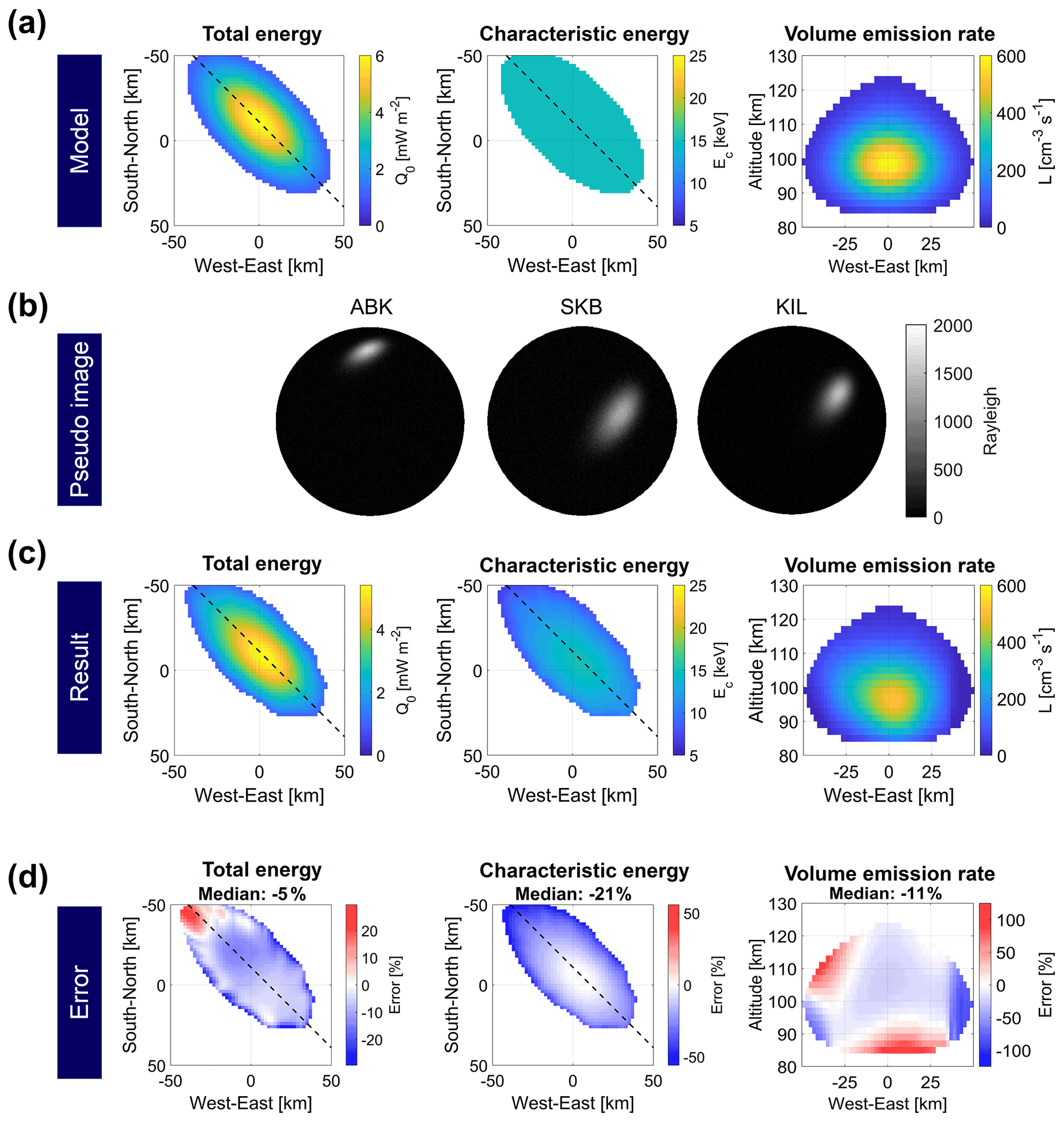
Figure 2 (a) The horizontal distribution of the prepared total energy (Q₀) and the characteristic energy (E_c) of precipitating electrons and the vertical cross section of the volume emission rate (L) along the dashed lines in the left and middle panels. We derived L from the prepared Q₀ and E_c values using the aurora emission model. Q₀ and E_c are not shown for Q₀ values less than 1 mW m⁻². (b) Pseudoauroral images obtained by line-integrating the volume emission rate (VER). (c) The horizontal distribution of Q₀ and E_c and the vertical cross section of L reconstructed by aurora computed tomography from the pseudoauroral images. (d) The errors of Q₀, E_c, and L, calculated as (Error) = [(Result) − (Model)] $/$ (Model) × 100.

The PsA patches shown in Fig. 1a are embedded in the background diffuse auroral emission. We found that a horizontally uniform diffuse aurora causes ambiguity in the reconstruction result because the altitude of the uniform auroral structure cannot be determined from the single-wavelength images. Thus, we subtracted the background emission from the images prior to ACT reconstruction. We created the background emission image by assuming the same value for all voxels. The background VER was taken to be 75 cm⁻³ s⁻¹, corresponding to the spatially averaged observed background emission intensity. In this analysis, we assumed that the diffuse aurora showed a uniform VER in all voxels; however, the VER of the diffuse aurora depends generally on the altitude. We note that the altitude dependence of the VER did not affect the analysis result. This is because the horizontal distribution of the background emission intensity (i.e., diffuse aurora) in the auroral image was dependent only on the zenith angle θ (∝cos θ). This distribution is not dependent on the altitude distribution of the VER if the VER is horizontally uniform.

3 Results and discussion

3.1 Reconstruction of a pulsating aurora patch model

We reconstructed a PsA patch model from pseudoauroral images to evaluate the analytical error of ACT before reconstructing the PsA patch from the observed auroral images. To create the pseudoauroral images, we prepared the horizontal distributions of the total energy (Q₀) and the characteristic energy (E_c). We then derived the 3-D VER (L), as shown in Fig. 2a. The total energy was assumed to have a Gaussian shape in the horizontal directions with a maximum value of 6 mW m⁻². The energy distribution was considered to be a Maxwellian distribution with a uniform characteristic energy of 15 keV. Pseudoauroral images were obtained from L by solving the forward problem (Fig. 2b). We added random noise from a normal distribution with a mean value of 0 and the standard deviation determined from observed auroral images.

Figure 2c shows Q₀, E_c, and L reconstructed from the pseudoauroral images. The values of Q₀ were calculated as $Q_{\mathrm{0}}={\sum }_i{E}_{i}f\left(E_i\right)\left(E_{i+\mathrm{1}}-E_i\right)$. When we assume the energy distribution to be a Maxwellian distribution, the characteristic energy can be written as $E_{\mathrm{c}}=\frac{\mathrm{1}}{\mathrm{2}}\langle E\rangle =\frac{\mathrm{1}}{\mathrm{2}}\frac{Q_{\mathrm{0}}}{{\sum }_{i}f\left(E_i\right)\left(E_{i+\mathrm{1}}-E_i\right)}$. We calculated the errors between the model and the result for Q₀, E_c, and L (Fig. 2d). The median values of the errors were −5 % for Q₀, −21 % for E_c, and −11 % for L. The northwestern part of Q₀ was overestimated by at most 23 %, the edge part was underestimated by at most 29 %, and the central part was underestimated by ∼ 8 %. The central part of E_c was reconstructed correctly. In comparison, the edge part (especially the northwestern part) was underestimated by at most 56 %. The underestimation of E_c was caused by the overestimation of the emission altitude (Fig. 2d). The information regarding the PsA emission altitude is easily lost in obtaining the auroral image, as the structure of the PsA patch is vertically thin and horizontally wide. In addition, the SNR in the edge part is lower than in the central part because we assumed a Gaussian shape for the horizontal distribution of Q₀. These factors would tend to reduce the accuracy in the edge part. In this particular event, the optical observation points of ABK, SKB, and KIL were located in the southeastern direction from the PsA patch at the EISCAT radar observation point (TRO) (see Fig. 1). Therefore, an accurate reconstruction of the VER peak altitude was more difficult in the northwestern part than in other parts. This was because of the insufficient information on the northwestern part of the PsA patch owing to the bias in the optical observation point distribution.

Notably, the reconstructed results using the hyperparameters determined by the cross-validation method revealed unexpected fine structures. To avoid this phenomenon, we set the lower limit of λ using a different method, namely by minimizing the sum of squares of the residuals between the model and the reconstructed result of Q₀ and E_c. The lower limit on λ makes it challenging to reconstruct actual fine-scale structures in the patches.

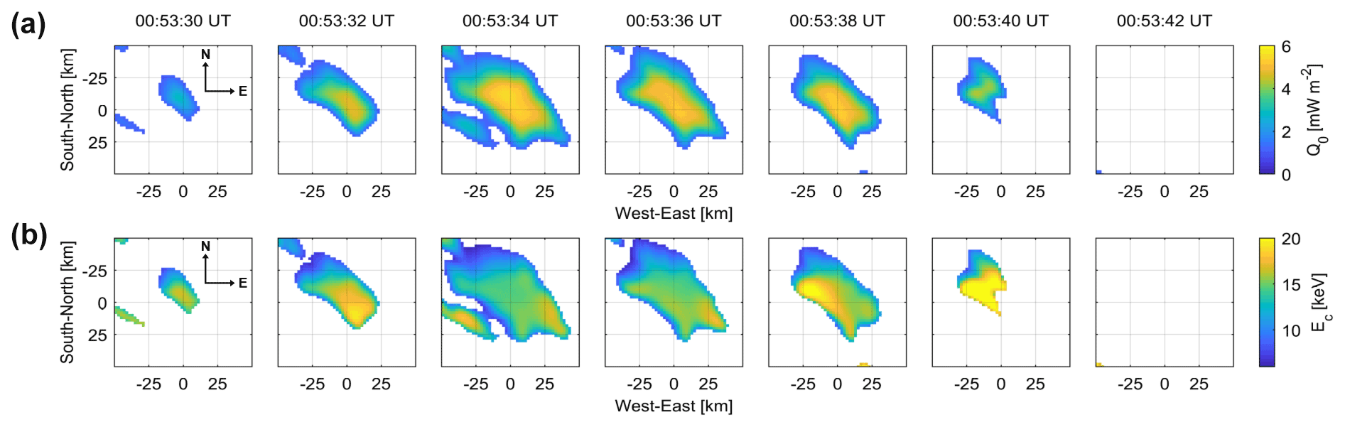
Figure 3 (a) Total energy (Q₀) and (b) characteristic energy (E_c) of the precipitating electron flux reconstructed from the observed auroral images. Results of Q₀ and E_c where Q₀ is less than 1 mW m⁻² are not shown.

3.2 Precipitating electrons

Figure 3a and b show Q₀ and E_c as reconstructed from the observed auroral images (Fig. 1a). The maximum value of Q₀ was ∼ 6 mW m⁻². The reconstructed E_c ranged from 6 to 23 keV. These energies are consistent with observation results from sounding rockets and low-altitude satellites (e.g., McEwen et al., 1981; Miyoshi et al., 2015). The horizontal distribution of E_c was neither uniform nor stable in the patch during the pulsation. Thus, the ACT method is helpful for investigating PsA-associated temporal variations in the horizontal distribution of precipitating electrons without rocket or satellite observations. In particular, the southwestern part of E_c was enhanced at 00:53:38 UT. It should be noted that the edge and in the northwestern parts of E_c are expected to be underestimated owing to analytical error, as shown in Fig. 2d. These temporal variations indicate changes in the cyclotron resonance energy of whistler-mode chorus waves during the pulsation. The chorus waves scatter electrons into a loss cone near the magnetic equator. The cyclotron resonance energy of chorus waves depends on the background magnetic field, electron density, and wave frequency (e.g., Kennel and Petschek, 1966). Therefore, the observed temporal variations indicate changes in the magnetospheric source region's background magnetic or plasma environment during the pulsation.

The characteristic energy can also be enhanced by the field-aligned current (FAC). The absence of the FAC in the PsA patch has been observed because the PsA patch has no shear motion and the energy spectra of precipitating electrons observed by rockets and satellites did not show a field-aligned acceleration, which are typically observed in discrete aurora (Davis, 1978). On the other hand, several studies have reported the FAC associated with PsA patches (Fujii et al., 1985; Gillies et al., 2015; Hosokawa and Ogawa, 2010). If the upward and downward FACs flow at the edge of the PsA path, the potential drop due to the upward FAC can accelerate precipitating electrons and enhance their characteristic energy (Sato et al., 2004; Shepherd and Fälthammar, 1980). However, we cannot suggest the existence of the FAC at the PsA patch's edge for this event because the total energy was not enhanced at the edge (Fig. 3). If the FAC exists, both total and characteristic energy should be increased. Multi-event analysis is needed to examine the FAC in PsA patches. The 3-D current structure in the PsA patch is beyond the scope of this study. Its reconstruction using ACT and EISCAT_3-D radar is planned in the future.

3.3 Volume emission rate

The 3-D distributions of the VERs derived from the reconstructed electron flux were obtained by solving the forward problem described in Sect. 2 (see Fig. 4a). Cross sections in the horizontal plane at an altitude of 94 km are shown in Fig. 4b. The peak altitude ranges from 90 to 104 km (Fig. 4c). The full width at half maximum is almost uniform with a median value of ∼ 20 km (Fig. 4e). The errors of the peak altitude and the altitude width in Fig. 4d and f were derived using the model and reconstructed VER shown in Fig. 2. The high peak altitude in the northwestern part is expected to be overestimated by at most 8 % owing to analytical error, as shown in Fig. 2d. For the altitude width, the most part is expected to be overestimated by ∼ 2 % (Fig. 4f). The reconstructed peak altitude and width are consistent with those determined in studies using stereoscopic observations or an incoherent scatter radar (Brown et al., 1976; Jones et al., 2009; Kataoka et al., 2016). Stenbaek-Nielsen and Hallinan (1979) reported the existence of thin (<1 km vertical extent) PsA patches based on stereoscopic observations, but our results do not support their results.

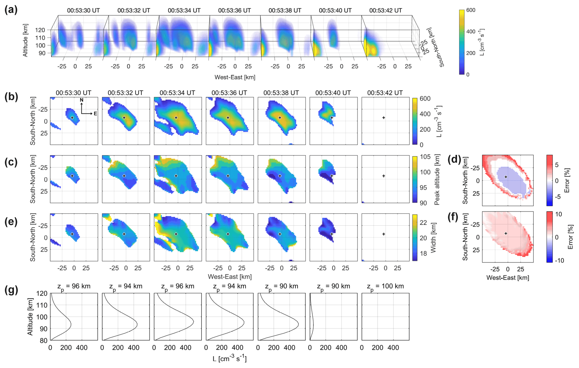
Figure 4 (a) Reconstructed 3-D distribution of volume emission rates (VERs), L. VERs less than 1 cm⁻³ s⁻¹ are not shown. (b) Cross sections in the horizontal plane at an altitude of 94 km. VERs are not shown for Q₀ values less than 1 mW m⁻². (c) Peak altitudes of the reconstructed L and (d) their errors determined using the model aurora. (e) Altitude widths of the reconstructed L and (f) their errors determined using the model aurora. (g) Altitude profiles of L at the European incoherent scatter radar observation point, as indicated by black plus marks in panels (b)–(f).

The peak altitude of the PsA patch was also estimated using a different method (Appendix A). We projected the observed auroral images at altitudes ranging from 80 to 120 km with an interval of 2 km (Video A1, https://doi.org/10.5446/57558). The emission altitude was determined to be the altitude at which the sum of squares of the residuals between the two projected images reached a minimum value (Fig. A1). The estimated peak altitude range was 92 to 106 km from 00:53:30 to 00:53:40 UT (Fig. A2). These altitudes closely match those determined by ACT.

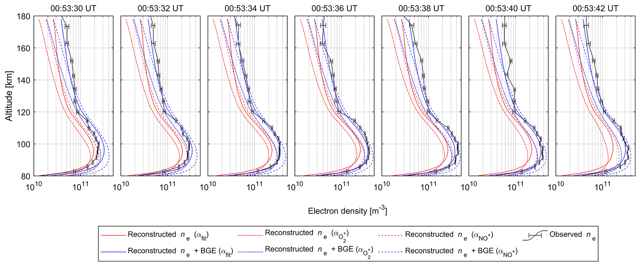
Figure 5 Electron density altitude profiles (n_e) converted from the reconstructed volume emission rates with the subtraction of the background emission (BGE) (red lines), those without the BGE subtraction (blue lines), and those observed by the European incoherent scatter radar (black lines). Details of effective recombination coefficients α_fit, ${\mathit{\alpha }}_{{\mathrm{O}}_{\mathrm{2}}^{+}}$, and ${\mathit{\alpha }}_{{\mathrm{NO}}^{+}}$ are explained in the text. The measurement uncertainties are represented by error bars.

3.4 Electron density

The altitude profiles of VER at the EISCAT radar observation point shown in Fig. 4g were converted to the ionospheric electron density and compared with the actual data observed by the EISCAT radar. The continuity equation for the electron density can be written as

$$\begin{array}{}\text{(4)}& {\displaystyle \frac{\partial n_{\mathrm{e}}}{\partial t}}=kL-{\mathit{\alpha }}_{\mathrm{eff}}{n}_{\mathrm{e}}^{\mathrm{2}},\end{array}$$

where n_e [m⁻³] is the electron density, L [m⁻³ s⁻¹] is the VER, k is a positive constant for converting VER to the ionization rate (see Appendix B), and α_eff [m³ s⁻¹] is the effective recombination rate. We derived the electron density from the VER by solving Eq. (4) with the Runge–Kutta method. The initial value was derived from Eq. (4) under steady-state conditions (i.e., $\partial n_{\mathrm{e}}/\partial t=\mathrm{0})$ using reconstructed L at 00:53:36 UT. The VERs were interpolated linearly in time to use the Runge–Kutta method. The altitude profile of α_eff has been investigated by several studies using rocket- and ground-based measurements. Vickrey et al. (1982) summarized many of these results and proposed the following best fit parameterization:

$$\begin{array}{}\text{(5)}& {\mathit{\alpha }}_{\mathrm{fit}}=\mathrm{2.5}\times {\mathrm{10}}^{-\mathrm{12}}\exp \left(-z/\mathrm{51.2}\right)\left[{\mathrm{m}}^{\mathrm{3}}{\mathrm{s}}^{-\mathrm{1}}\right],\end{array}$$

where z [km] is the altitude. Semeter and Kamalabadi (2005) used the effective recombination coefficients ${\mathit{\alpha }}_{{\mathrm{NO}}^{+}}$ and ${\mathit{\alpha }}_{{\mathrm{O}}_{\mathrm{2}}^{+}}$ for NO⁺ and O${}_{\mathrm{2}}^{+}$, respectively (Walls and Dunn, 1974), as upper and lower bounds on α_eff:

$$\begin{array}{}\text{(6)}& {\displaystyle }{\mathit{\alpha }}_{{\mathrm{NO}}^{+}}=\mathrm{4.2}\times {\mathrm{10}}^{-\mathrm{13}}{\left(\mathrm{300}/T_{\mathrm{n}}\right)}^{\mathrm{0.85}}\left[{\mathrm{m}}^{\mathrm{3}}{\mathrm{s}}^{-\mathrm{1}}\right],\text{(7)}& {\displaystyle }{\mathit{\alpha }}_{{\mathrm{O}}_{\mathrm{2}}^{+}}=\mathrm{1.95}\times {\mathrm{10}}^{-\mathrm{13}}{\left(\mathrm{300}/T_{\mathrm{n}}\right)}^{\mathrm{0.7}}\left[{\mathrm{m}}^{\mathrm{3}}{\mathrm{s}}^{-\mathrm{1}}\right].\end{array}$$

Here, T_n [K] is the neutral temperature. The red lines in Fig. 5 show the derived electron densities using these three recombination coefficients. We note that these values are underestimated compared with the electron densities observed by the EISCAT radar (black lines in Fig. 5). This underestimation probably comes from the background emission subtraction from the auroral images prior to ACT and from ambiguity in the effective recombination coefficients. The electron densities reconstructed from auroral images without background emission subtraction are shown as blue lines for reference in Fig. 5. The reconstruction results from the images, including background emission, approached the electron density profile observed with the EISCAT radar. We note that the electron density was reconstructed correctly to some extent, even after the auroral emission intensity decreased at 00:53:40 UT. This correct reconstruction considered the time change in the continuity equation. The electron density would seem to have rapidly decreased after 00:53:40 UT if the time change was not considered. This result suggested that the time change should be considered ($\mathrm{d}{n}_{\mathrm{e}}/\mathrm{d}t\ne \mathrm{0}$ in Eq. 4) when using the continuity equation to derive the electron densities associated with PsAs.

It should be noted that the electron density is underestimated at higher altitudes (> ∼ 140 km), even if the background emission is included. This underestimation can be improved by reconstructing low-energy electron flux from auroral images of various wavelengths (e.g., 844.6 nm).

4 Conclusions

We applied the ACT method to a PsA patch for the first time and reconstructed the horizontal distribution of precipitating electrons from 427.8 nm auroral images obtained from three observation points. We improved the previously proposed ACT method by adding the following processes: the subtraction of the background diffuse aurora from the auroral images prior to ACT, the estimation of the relative sensitivity between ASCs, and the determination of the hyperparameters of the regularization term. The characteristic energies of the reconstructed electron fluxes (6 to 23 keV) and the peak altitudes of the reconstructed VERs (90 to 104 km) were consistent with those found in previous studies. We determined that the horizontal distribution of the characteristic energy was neither uniform nor stable in the patch during the pulsation, further underlining the shortcomings of rocket and satellite observations with respect to investigating PsAs. These spatial and temporal variations imply changes in the electron density and magnetic field in the magnetosphere. ACT error was evaluated using an auroral patch model. The characteristic energy of electron flux was correctly reconstructed in the center part of the patch but underestimated at the patch edge by at most 56 %. The reconstructed electron flux will be improved in future work by incorporating auroral images of various wavelengths.

Although we reconstructed the differential flux of precipitating electrons from auroral images using ACT, Tanaka et al. (2011) extended ACT to a method called generalized-aurora computed tomography (G-ACT). G-ACT uses multi-instrument data, such as ionospheric electron density from incoherent scatter radar, cosmic noise absorption from imaging riometers, and the auroral images. Tanaka et al. (2011) demonstrated that the incorporation of the ionospheric electron density from the EISCAT radar improved the accuracy of the reconstructed electron flux. Furthermore, 3-D ionospheric observation by EISCAT_3-D (http://www.eiscat3d.se, last access: 7 July 2022) is scheduled to begin in 2023. In the future, we will improve the reconstructed electron flux by conducting G-ACT analysis using electron density data from the EISCAT or EISCAT_3-D radar.

Appendix A: Estimation of the pulsating auroral emission peak altitude

Here, we estimate the peak altitude of the PsA patch using a different method to validate the results from ACT in Sect. 3.3. We projected the observed auroral images at altitudes from 80 to 120 km with an interval of 2 km. As an example, projected images for 00:53:36 UTC on 18 February 2018 are shown in Video A1 (https://doi.org/10.5446/57558). The emission altitude was determined to be the altitude at which the sum of squares of the residuals of the auroral intensity between the two projected images reached a minimum value (Fig. A1). The estimated peak altitudes from 00:53:30 to 00:53:40 UTC are shown in Fig. A2. These altitudes agreed with the results from ACT in Sect. 3.3.

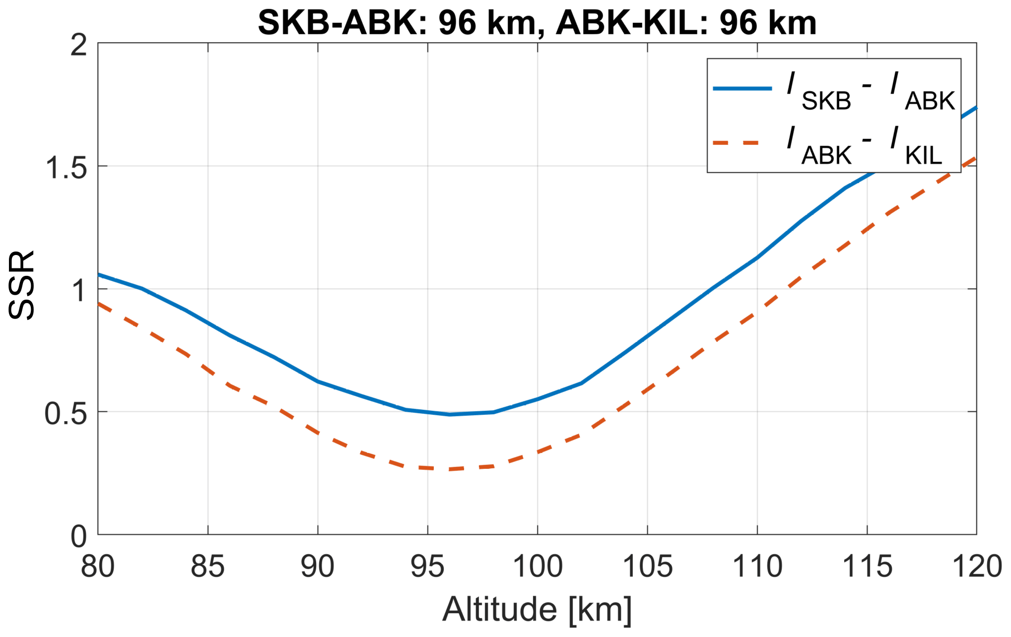
Figure A1 The sum of squares of the residuals (SSR) between the projected images at two stations (SKB and ABK, and ABK and KIL) at each altitude at 00:53:36 UT on 18 February 2018. The altitude at which the SSR reached a minimum value is shown in the panel title.

Figure A2 The altitude at which the sum of squares of the residuals (SSR) reached a minimum value for each of six time points from 00:53:30 to 00:53:40 UT on 18 February 2018. Error bars indicate the altitude range over which the SSR was less than 1.2 times each SSR minimum.

Appendix B: Derivation of k

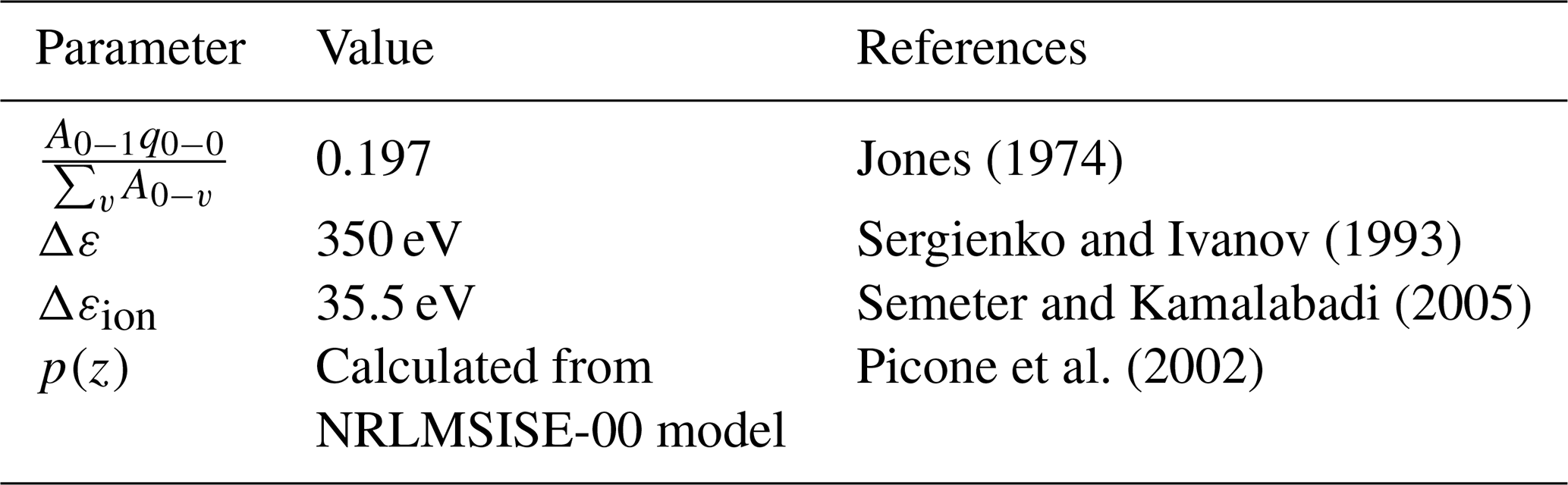
In this section, we describe how to obtain the positive constant k(z) from Sect. 3.4. The ${\mathrm{N}}_{\mathrm{2}}^{+}$ (427.8 nm) emission is owing to the transition from ${\mathrm{N}}_{\mathrm{2}}^{+}{\left(B^{\mathrm{2}}{\mathbf{\Sigma }}_u^{+}\right)}_{v=\mathrm{0}}$ to ${\mathrm{N}}_{\mathrm{2}}^{+}{\left(X^{\mathrm{2}}{\mathbf{\Sigma }}_g^{+}\right)}_{v=\mathrm{1}}$. According to Sergienko and Ivanov (1993), the VER L(z) [m⁻³s⁻¹] is approximated by

$$\begin{array}{}\text{(B1)}& L\left(z\right)={\displaystyle \frac{A_{\mathrm{0}-\mathrm{1}}{q}_{\mathrm{0}-\mathrm{0}}}{{\sum }_v{A}_{\mathrm{0}-v}}}w\left(z\right)={\displaystyle \frac{A_{\mathrm{0}-\mathrm{1}}{q}_{\mathrm{0}-\mathrm{0}}}{{\sum }_v{A}_{\mathrm{0}-v}}}{\displaystyle \frac{p\left(z\right)\mathit{\epsilon }\left(z\right)}{\mathrm{\Delta }\mathit{\epsilon }}},\end{array}$$

where A₀₋₁ is the Einstein coefficient for the transition from ${\mathrm{N}}_{\mathrm{2}}^{+}{\left(B^{\mathrm{2}}{\mathbf{\Sigma }}_u^{+}\right)}_{v=\mathrm{0}}$ to ${\mathrm{N}}_{\mathrm{2}}^{+}{\left(X^{\mathrm{2}}{\mathbf{\Sigma }}_g^{+}\right)}_{v=\mathrm{1}}$, w(z) [m⁻³ s⁻¹] is the production rate of ${\mathrm{N}}_{\mathrm{2}}^{+}\left(B^{\mathrm{2}}{\mathbf{\Sigma }}_u^{+}\right)$, q₀₋₀ is the Franck–Condon factor for the electronic transition from ${\mathrm{N}}_{\mathrm{2}}^{+}{\left(X^{\mathrm{1}}{\mathbf{\Sigma }}_g^{+}\right)}_{v=\mathrm{0}}$ to ${\mathrm{N}}_{\mathrm{2}}^{+}{\left(B^{\mathrm{2}}{\mathbf{\Sigma }}_u^{+}\right)}_{v=\mathrm{0}}$, p(z) is the probability that ε(z) excites N₂, ε(z) [eV m⁻³ s⁻¹] is the energy deposition rate, and Δε [eV] is the excitation energy cost of ${\mathrm{N}}_{\mathrm{2}}^{+}\left(B^{\mathrm{2}}{\mathbf{\Sigma }}_u^{+}\right)$. The ionization rate due to the precipitating electrons q_ion(z) [m⁻³ s⁻¹] is given by

$$\begin{array}{}\text{(B2)}& q_{\mathrm{ion}}\left(z\right)={\displaystyle \frac{\mathit{\epsilon }\left(z\right)}{\mathrm{\Delta }{\mathit{\epsilon }}_{\mathrm{ion}}}},\end{array}$$

where Δε_ion [eV] is the energy used to produce an ion–electron pair. Substituting Eq. (B1) into Eq. (B2) gives

$$\begin{array}{}\text{(B3)}& q_{\mathrm{ion}}\left(z\right)={\displaystyle \frac{\sum _v{A}_{\mathrm{0}-v}}{A_{\mathrm{0}-\mathrm{1}}{q}_{\mathrm{0}-\mathrm{0}}}}{\displaystyle \frac{\mathrm{\Delta }\mathit{\epsilon }}{\mathrm{\Delta }{\mathit{\epsilon }}_{\mathrm{ion}}}}{\displaystyle \frac{\mathrm{1}}{p\left(z\right)}}L\left(z\right).\end{array}$$

Therefore, the positive constant k(z) for converting VER to the ionization rate is

$$\begin{array}{}\text{(B4)}& k\left(z\right)={\displaystyle \frac{{\sum }_v{A}_{\mathrm{0}-v}}{A_{\mathrm{0}-\mathrm{1}}{q}_{\mathrm{0}-\mathrm{0}}}}{\displaystyle \frac{\mathrm{\Delta }\mathit{\epsilon }}{\mathrm{\Delta }{\mathit{\epsilon }}_{\mathrm{ion}}}}{\displaystyle \frac{\mathrm{1}}{p\left(z\right)}}.\end{array}$$

The parameters used for the calculation are summarized in Table B1.

Table B1 Simulation parameters used in Eq. (B4).