the Creative Commons Attribution 4.0 License.
the Creative Commons Attribution 4.0 License.
 | 09 May 2022
Menura: a code for simulating the interaction between a turbulent solar wind and solar system bodies
Shahab Fatemi
Pierre Henri
Mats Holmström
Despite the close relationship between planetary science and plasma physics, few advanced numerical tools allow bridging the two topics. The code Menura proposes a breakthrough towards the self-consistent modelling of these overlapping fields, in a novel two-step approach allowing for the global simulation of the interaction between a fully turbulent solar wind and various bodies of the solar system. This article introduces the new code and its two-step global algorithm, illustrated by a first example: the interaction between a turbulent solar wind and a comet.
- Article
(11047 KB) - Full-text XML
- BibTeX
- EndNote


For about a century, three main research fields have taken an interest in the various space plasma environments found around the Sun. On the one hand, two of them, namely planetary science and solar physics, have been exploring the solar system, to understand the functioning and history of its central star, and of its myriad of orbiting bodies. On the other hand, the third one, namely fundamental plasma physics, has been using the solar wind as a handy wind tunnel which allows researchers to study fundamental plasma phenomena not easily reproducible on the ground, in laboratories. During the last decades, the growing knowledge of these communities has led them to research on ever more overlapping topics. For instance, planetary scientists were initially studying the interaction between solar system bodies and a steady, ideally laminar solar wind, but they soon had to consider its eventful and turbulent nature to go further in the in situ space data analysis, further in their understanding of the interactions at various obstacles. Similarly, plasma physicists were originally interested in a pristine solar wind unaffected by the presence of obstacles. They however realised that the environment close to these obstacles could provide combinations of plasma parameters otherwise not accessible to their measurements in the unaffected solar wind. For a while now, we have seen planetary studies focusing on the effects of solar wind transient effects (such as coronal mass ejection, CME, or co-rotational interaction region, CIR) on planetary plasma environments, on Mars (Ramstad et al., 2017), Mercury (Exner et al., 2018), Venus (Luhmann et al., 2008) and comet 67P/C-G (Edberg et al., 2016; Hajra et al., 2018) to only cite a few, the effect of large-scale fluctuations in the upstream flow on Earth's magnetosphere (Tsurutani and Gonzalez, 1987), and more generally the effect of solar wind turbulence on Earth's magnetosphere and ionosphere (D'Amicis et al., 2020; Guio and Pécseli, 2021). Similarly, plasma physicists have developed comprehensive knowledge of plasma waves and plasma turbulence in the Earth's magnetosheath, presenting relatively high particle densities and electromagnetic field strengths, favourable for space instrumentation, and in a region more easily accessible to space probes than regions of unaffected solar wind (Borovsky and Funsten, 2003; Rakhmanova et al., 2021). More recently, the same community took an interest in various planetary magnetospheres, depicting plasma turbulence in various locations and of various parameters (Saur, 2021, and all references therein).
Various numerical codes have been used for the global simulation of the interaction between a laminar solar wind and solar system bodies, using MHD (Gombosi et al., 2004), hybrid (Bagdonat and Motschmann, 2002), or fully kinetic (Markidis et al., 2010) solvers. Similarly, solar wind turbulence in the absence of an obstacle has also been simulated using similar MHD (Boldyrev et al., 2011), hybrid (Franci et al., 2015), and fully kinetic (Valentini et al., 2007) solvers. In this context, we identify the lack of a numerical approach for the study of the interaction between a turbulent plasma flow (such as the solar wind) and an obstacle (such as a magnetosphere, either intrinsic or induced). Such a tool would provide the first global picture of these complex interactions. By shedding light on the long-lasting dilemma between intrinsic phenomena and phenomena originating from the upstream flow, it would allow invaluable comparisons between self-consistent, global, numerical results, and the worth of observational results provided by the various past, current and future exploratory space missions in our solar system.
The main points of interest and main questions motivating such a model can be organised as such:
- –
macroscopic effects of turbulence on the obstacle
- –
shape and position of the plasma boundaries (e.g. bow shock, magnetopause),
- –
large-scale magnetic reconnection,
- –
atmospheric escape,
- –
dynamical evolution of the magnetosphere.
- –
- –
microscopic physics and instabilities within the interaction region, induced by upstream turbulence
- –
energy transport by plasma waves,
- –
energy conversion by wave–particle interactions,
- –
energy transfers by instabilities.
- –
- –
the way incoming turbulence is processed by planetary plasma boundaries
- –
sudden change of spatial and temporal scales,
- –
change of spectral properties,
- –
existence of a memory of turbulence downstream magnetospheric boundaries.
- –
Indirectly, because of the high numerical resolution required to properly simulate plasma turbulence, this numerical experiment will provide an exploration of the various obstacles with the same high resolution in both turbulent and laminar runs, resolutions that have rarely been reached for planetary simulations, except for Earth's magnetosphere.
Menura, the new code presented in this publication, splits the numerical modelling of the interaction into two steps. Step 1 is a decaying turbulence simulation, in which electromagnetic energies initially injected at the large spatial scales of the simulation box cascades towards smaller scales. Step 2 uses the output of Step 1 to introduce an obstacle moving through this turbulent solar wind.
The code is written in C++ and uses CUDA APIs for running its solver exclusively on multiple graphics processing units (GPUs) in parallel. Section 2 introduces the solver, which is tested against classical plasma phenomena in Sect. 3. Sections 4 and 5 tackle the first and second step of the new numerical modelling approach, illustrating the decaying turbulence phase, and introducing the algorithm for combining the output of Step 1 together with the modelling of an obstacle (Step 2). Section 6 presents the first global result of Menura, providing a glimpse of the potential of this numerical approach, and introducing the forthcoming studies.
Menura source code is open source, available under the GNU General Public License.
In order to (i) achieve global simulations of the interactions while (ii) modelling the plasma kinetic behaviour, with regard to the computation capabilities currently available, a hybrid particle-in-cell (PIC) solver has been chosen for Menura. This well-established type of model resolves the Vlasov equation for the ions by discretising the ion distribution function as macroparticles characterised by discrete positions in phase space, and electrons as a fluid, with characteristics evaluated at the nodes of a grid, together with ion moments and electromagnetic fields. The fundamental computational steps of a hybrid PIC solver are the following:
-
particles' position advancement, or “push”;
-
particles' moments mapping, or “gathering”: density, current, eventually higher order, as required by the chosen Ohm's law;
-
electromagnetic field advancement, using either an ideal, resistive or generalised Ohm's law and Faraday's law;
-
Particles' velocity advancement, or “push”.
These steps are summarised in Fig. 1. Details about these classical principles can be found in Tskhakaya (2008) and references therein. The bottleneck of PIC solvers is the particles' treatment, especially the velocity advancement and the moments computation (namely density and current). The simulation of plasma turbulence especially requires large numbers of macroparticles per grid node. We therefore want to minimise both the number of operations done on the particles and the number of particles itself. A popular method which minimises the number of these computational passes through all particles is the current advance method (CAM) (Matthews, 1994), for instance used for the hybrid modelling of turbulence by Franci et al. (2015). Figure 1 presents Menura's solver algorithm, built around the CAM, similar to the implementation of Bagdonat and Motschmann (2002). In this scheme, only four passes through all particles are performed, one position and one velocity pushes and two particle moments mappings. The second moment mapping in Fig. 1, i.e. Step 2, also produces the two pseudo-moments Λ and Γ used to advance the current as follows:
with E* the estimated electric field after the magnetic field advancement of Step 4. W(rn+1) is the shape function, which attributes different weights for each node surrounding the macroparticle (Tskhakaya, 2008).
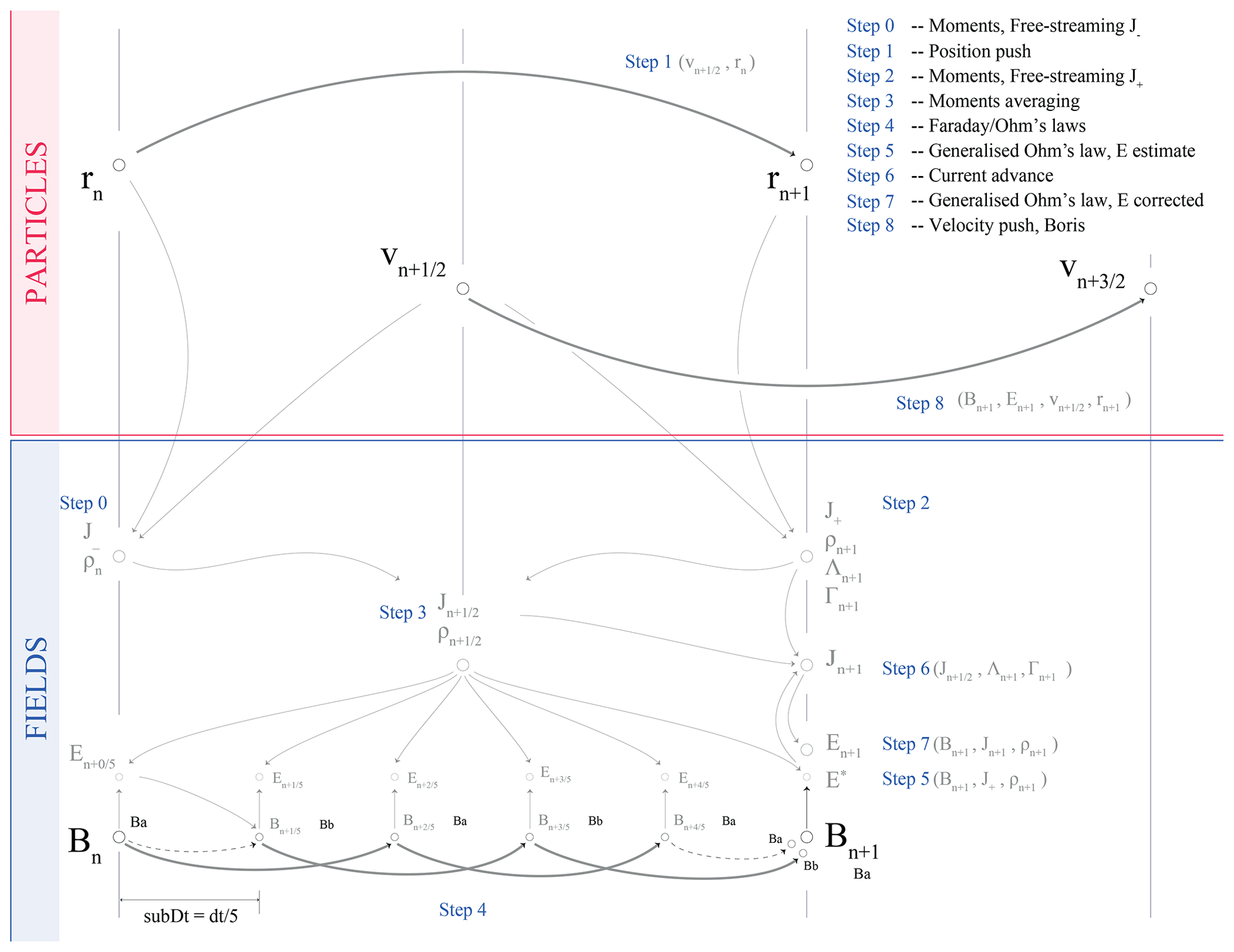
Figure 1Algorithm of Menura's solver, with its main operations numbered from 0 to 8, as organised in the main file of the code. r and v are the position and velocity vectors of the macroparticles. Together with the magnetic field B, they are the only variables necessary for the time advancement. The electric field E, the current J, and the charge density ρ, as well as the CAM pseudo-moments Λ and Γ, are obtained from r, v and B.
Central finite differences using a five-point stencil for evaluating derivatives as well as second-order interpolations are used throughout the solver. The algorithm evaluates all fields values at the nodes (or equivalently cell centres in this precise case) of the grid. In Appendix B, we discuss how such a scheme actually conserves , as initially shown by Tóth (2000). Additionally, Appendix B illustrates the evolution of the total energy of the system.
The grid covering the physical simulation domain has an additional two-node wide band, the guard or ghost nodes, allowing one to solve derivatives using (central) finite differences at the very edge of the physical domain. For periodic boundary conditions, as used along all directions during Step 1 of the simulation, the values at the opposite edge of the physical domain are copied to the guard nodes. Other boundary conditions will be discussed later when introduced.
The mapping of the particle moments is done using an order-two, triangular shape function: one macroparticle contributes to 9 grid nodes in 2D space (respectively 27 in 3D space), using 9 (respectively 27) different weights. The interpolation of the field values from the nodes to the macroparticles' positions uses the exact same weights, with 9 (respectively 27) neighbouring nodes contributing to the fields values at a particle position.
As illustrated in Fig. 1, the position and velocity advancements are done at interleaved times, similarly as a classical second-order leap-frog scheme. However, since the positions of the particles are needed to evaluate their acceleration, the CAM scheme is not strictly speaking a leap-frog integration scheme. Another difference in this implementation is that velocities are advanced using the Boris method (Boris, 1970).
Ohm's law is at the heart of the hybrid modelling of plasmas. Menura uses the following form of the law, here given in SI units. In this formulation, the electron inertia is neglected, and the quasi-neutral approximation is used (Valentini et al., 2007). Additionally, neglecting the time derivative of the electric field in Ampere–Maxwell's law (Darwin's hypothesis), one gets the total current through the curl of the magnetic field. This formulation highlights the need for only three types of variables to be followed through time, namely the magnetic field, and the particles position and velocity, while all other variables can be reconstructed from these three.
Faraday's law is used for advancing the magnetic field in time:
The electron pressure is obtained assuming it results from a polytropic process, with an arbitrary index κ, to be chosen by the user. In all the results presented below, an index of 1 was used, corresponding to an isothermal process.
Using much less memory than the particles' variables, the fields can be advanced in time using a smaller time step and another leap-frog-like approach, as illustrated in Fig. 1, Step 4 (Matthews, 1994).
Additional spurious high-frequency oscillations are the default behaviour of finite differences schemes. Two main families of methods are used to filter out these features, the first being an additional step of field smoothing, the second using the direct inclusion of a diffusive term in the differential equation of the system, acting as a filter (Maron et al., 2008). For Menura, we have retained the second approach, implementing a term of hyper-resistivity in Ohm's law, introducing the Laplacian of the total current and the hyper-resistivity coefficient, ηh∇2J. The dissipative scale Ldis of such a term is characterised by the physical time of the simulation and the resistivity, such as .
The stability of hybrid solvers is sensitive to low ion densities. We use a threshold value equal to a few percent of the background density, 5 % in the following examples, threshold below which a node is considered as a vacuum node, and only the resistive terms of the generalised Ohm's law of Eq. (4) are solved using a higher value of resistivity ηh vacuum (Holmström, 2013). This way, terms proportional to do not exhibit nonphysical values where the density may get locally very low, due to the thermal noise of the PIC macroparticle discretisation.
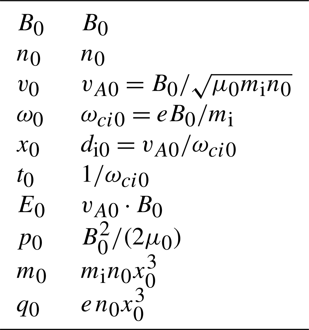
All variables in the code are normalised using the background magnetic field amplitude B0 and the background plasma density n0. All variables are then expressed in terms of either these two background values, or equivalently in terms of the proton gyrofrequency ωci0 and the Alfvén velocity vA0. We define normalised variables as obtained by dividing its physical value by its “background” value:
All background values are given in Table 1, and the normalised equations of the solver are given in Appendix A.
Table 1Background values used to normalise all variables in the solver (cf. Eq. 7).
In this section, the code is tested against well-known, collisionless plasma processes, and their solutions are given by the linear full kinetic solver WHAMP (Rönnmark, 1982). A polytropic index of 1 is used here, with no resistivity. We first explore MHD scales, simulating Alfvénic and magnetosonic modes. We use a 2-dimensional spatial domain with one preferential dimension chosen as x. A sum of six cosine modes in the component of the magnetic field along the x direction are initialised, corresponding to the first six harmonics of this periodic box. The amplitude of these modes is 0.05 times the background magnetic field B0, which is taken either along (Alfvén mode) or across (magnetosonic mode) the propagation direction x. Data are recorded along time and along the main spatial dimension x (saving one cut, given by one single index along the y direction), resulting in the 2D field B(x,t). The 2-dimensional Fourier transform of this field is given in Fig. 2 (Alfvénic fluctuations to the left, magnetosonic to the right). On this (ω,k) plane, each mode can be identified as a point of higher power, six points for six initial modes. The solutions given by WHAMP for the same plasma parameters are shown by the solid lines, and a perfect match is found between the two models. Close to the ion scale , WHAMP and Menura display two different branches that originate from the Alfvén mode, splitting for higher frequencies into the whistler and the ion cyclotron branches. The magnetosonic modes were also tested using a different polytropic index of instead of 1, resulting in a shift of the dispersion relation along the ω axis. Changing the polytropic index in both Menura and WHAMP resulted in the same agreement.

Figure 2MHD modes dispersion relations, as solved by WHAMP and Menura. B0=1.8 nT, n0=1.0 cm−3, Ti0=104 K, Te0=105 K. (a) Alfvénic modes, B0 taken along the main spatial dimension. (b) Magnetosonic modes, B0 taken perpendicular to the main spatial dimension.
With the MHD scales down to ion inertial scales now validated, we explore the ability of the solver to account for further ion kinetic phenomena, first with the classical case of the two-stream instability (also known as the ion-beam instability, given the following configuration). Two Maxwellian ion beams are initialised propagating with opposite velocities along the main dimension x. A velocity separation of 15 vth (the ion thermal speed) is used in order to excite only one unstable mode. The linear kinetic solver WHAMP is used to identify the expected growth rate associated with the linear phase of the instability, before both beams get strongly distorted and mixed in phase space during the nonlinear phase of the instability (not captured by WHAMP). During this linear phase, Menura results in a growing circularly polarised wave, and the amplitude's growth of the wave is shown in Fig. 3. Both growth rates match perfectly.
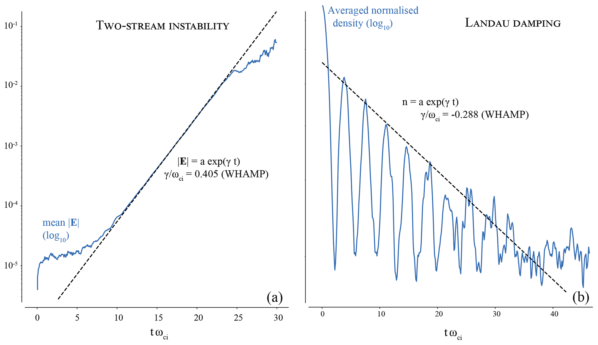
Figure 3(a) Growth during the linear phase of the ion–ion two-stream instability; (b) Landau damping of an ion acoustic mode. Two-stream instability: B0=1.8 nT, n0=1.0 cm−3, Ti0=102 K, Te0=103 K. Landau damping: B0=1.8 nT, n0=5.0 cm−3, K, Te0=105 K
Finally, we push the capacities of the model to the case of the damping of an ion acoustic wave through Landau resonance. A very high number of macroparticles per grid node is required to resolve this phenomenon, so enough resonant particles take part in the interaction with the wave. The amplitude of the initial, single acoustic mode is taken as 0.01 times the background density, taken along the main spatial dimension of the box. This low amplitude, allowing for comparison with the linear solver, further increases the need for a high number of particle per node, so the 1 % oscillation in number density can be resolved by the finite number of particles. For this run, 32 768 (215) particles per grid node were used. The decrease in the density fluctuation through time, spatially averaged, is shown in Fig. 3, with again the corresponding solution from WHAMP. A satisfying agreement is found during the first six oscillations, before the noise in the hybrid solver output (likely associated with the macroparticle thermal noise) takes over. Admittedly, the number of particles per node necessary to well resolve this phenomenon is not practical for the global simulations which Menura (together with all global PIC simulations) aims for.
For the classical tests presented above, spanning over MHD and ion kinetic scales tests, Menura agrees with theoretical and linear results. In the next section, the simulation of a decaying turbulent cascade provides one final physical validation of the solver, through all these scales at once.
We use Menura to simulate plasma turbulence using a decaying turbulent cascade approach: at initial time t=0, a sum of sine modes with various wave vectors k, spanning over the largest spatial scales of the simulation domain, are added to both the homogeneous background magnetic field B0 and the ion bulk velocity ui. Particle velocities are initialised according to a Maxwellian distribution, with a thermal speed equal to one Alfvén speed, and a bulk velocity given by the initial fluctuation. Without any other forcing later on, this initial energy cascades, as time advances, towards lower spatial and temporal scales, forming vortices and reconnecting current sheets (Franci et al., 2015). Using such Alfvénic perturbation is motivated by the predominantly Alfvénic nature of the solar wind turbulence measured at 1 au (Bruno and Carbone, 2013).
In this 2-dimensional set-up, B0 is taken along the z direction, perpendicular to the simulated spatial domain (x,y), whereas all initial perturbations are defined within the simulation plane. Their amplitude is 0.5 B0, while their wave vectors are taken with values between and , so energy is only injected in MHD scales, in the inertial range (Kiyani et al., 2015). Because we need these perturbation fields to be periodic along both directions, the kx and ky of each mode corresponds to harmonics of the simulation box dimensions. Therefore, a finite number of wave vector directions is initialised. Along these constrained directions, each mode in both fields has two different, random phases. The magnetic field is initialised such that is it divergence-free.
For this example, the box is chosen to be 500 di0 wide on both dimensions, subdivided by a grid 10002 nodes wide. The corresponding Δx is 0.5 di0, and spatial frequencies are resolved over the range [0.0062, 6.2] . The time step is 0.05 ; 2000 particles per grid node are initialised with a thermal speed of 1 vA. The temperature is isotropic and a plasma beta of 1 is chosen for both the ion macroparticles and the electronic massless fluid. The polytropic index is 1 and a normalised hyper-resistivity of is used, corresponding to a dissipative scale at time of 1. di0, i.e. the scale of the smallest fluctuations simulated with a node spacing of Δx=0.5di0.
At time , the perpendicular (in-plane) fluctuations of the magnetic field reached the state displayed in Fig. 4, left-hand panel. Vortices and current sheets give a maximum of about 1, a result consistent with solar wind turbulence observed at 1 au (Bruno and Carbone, 2013). The omni-directional power spectra of both the in-plane magnetic field fluctuations and the in-plane ion bulk velocity fluctuations are shown in the right-hand panel of the same figure. Omni-directional spectra are computed as follows, with the (2D) Fourier transform of f:
These spectra are not further normalised and are given in arbitrary units. We then compute a binned statistics over this 2-dimensional array to sum up its values within the chosen bins of k⟂, which correspond to rings in the (kx,ky) plane. The width of the rings, constant through all scales, is arbitrarily chosen so the resulting 1-dimensional spectrum is well resolved (not too few bins), and not too noisy (not too many bins).
For a vector field such as , the spectrum is computed as the sum of the spectra of each field component:
The perpendicular magnetic and kinetic energy spectra exhibit power laws over the inertial (MHD) range consistent with spectral indexes and , respectively, between and break points around 0.5 . We remind that a spectral index is consistent with the Goldreich–Sridhar strong turbulence phenomenology (Goldreich and Sridhar, 1997) that leads to a Kolmogorov-like scaling in the plane perpendicular to the background magnetic field, while a spectral index is consistent with the Iroshnikov–Kraichnan scaling (Kraichnan, 1965). These spectral slopes are themselves consistent with observations of magnetic and kinetic energy spectra associated with solar wind turbulence (Podesta et al., 2007; Chapman and Hnat, 2007). For higher wavenumbers, both spectral slopes get much steeper, and after a transition region within [0.5, 1.0] get to a value of about −3.2 and −4.5 when reaching the proton kinetic scales for respectively the perpendicular magnetic and kinetic energies, consistent with spectral index found at sub-ion scales by previous authors (Franci et al., 2015; Sahraoui et al., 2010, e.g.). Additionally, the initial spectra of the magnetic field and bulk velocity perturbations are over-plotted, to show where the energy is injected in the lower spatial frequencies (using the magnetic field fluctuations), and the level of noise introduced by the finite number of particles per node used, at high frequencies (using the bulk velocity field).
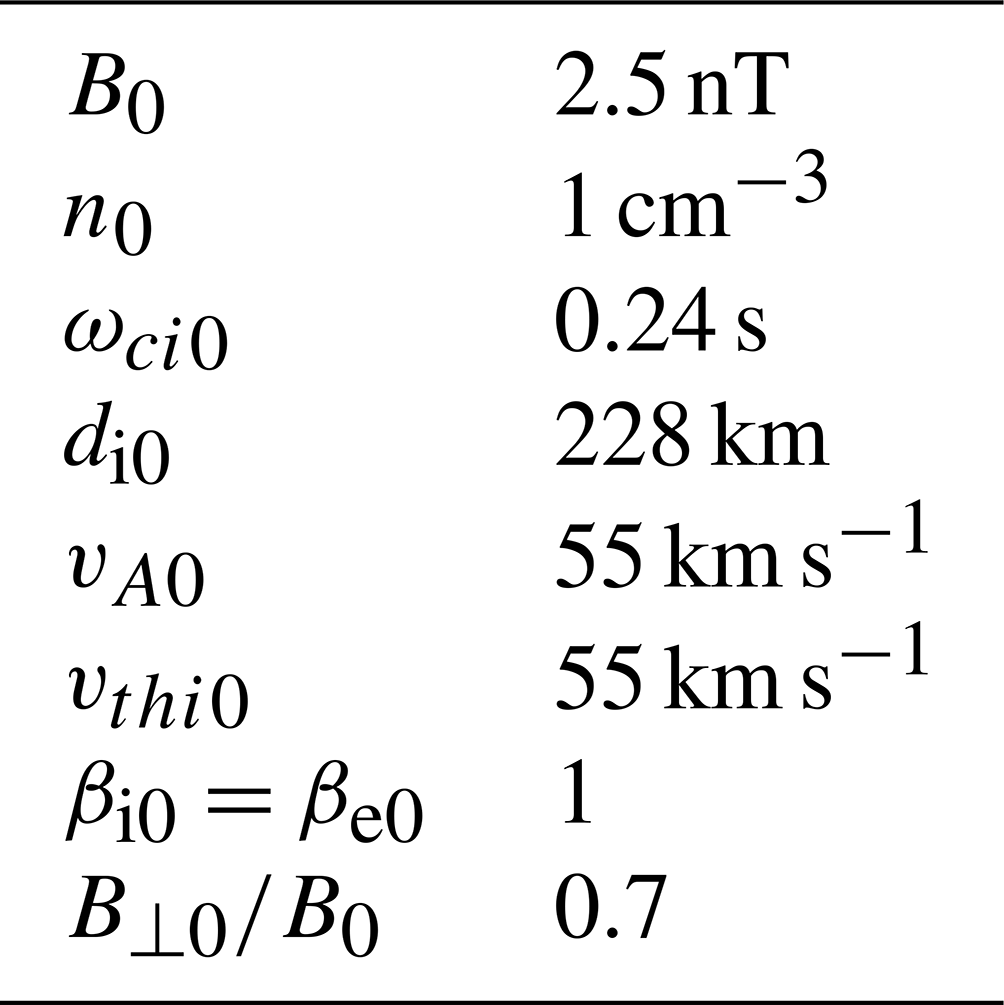
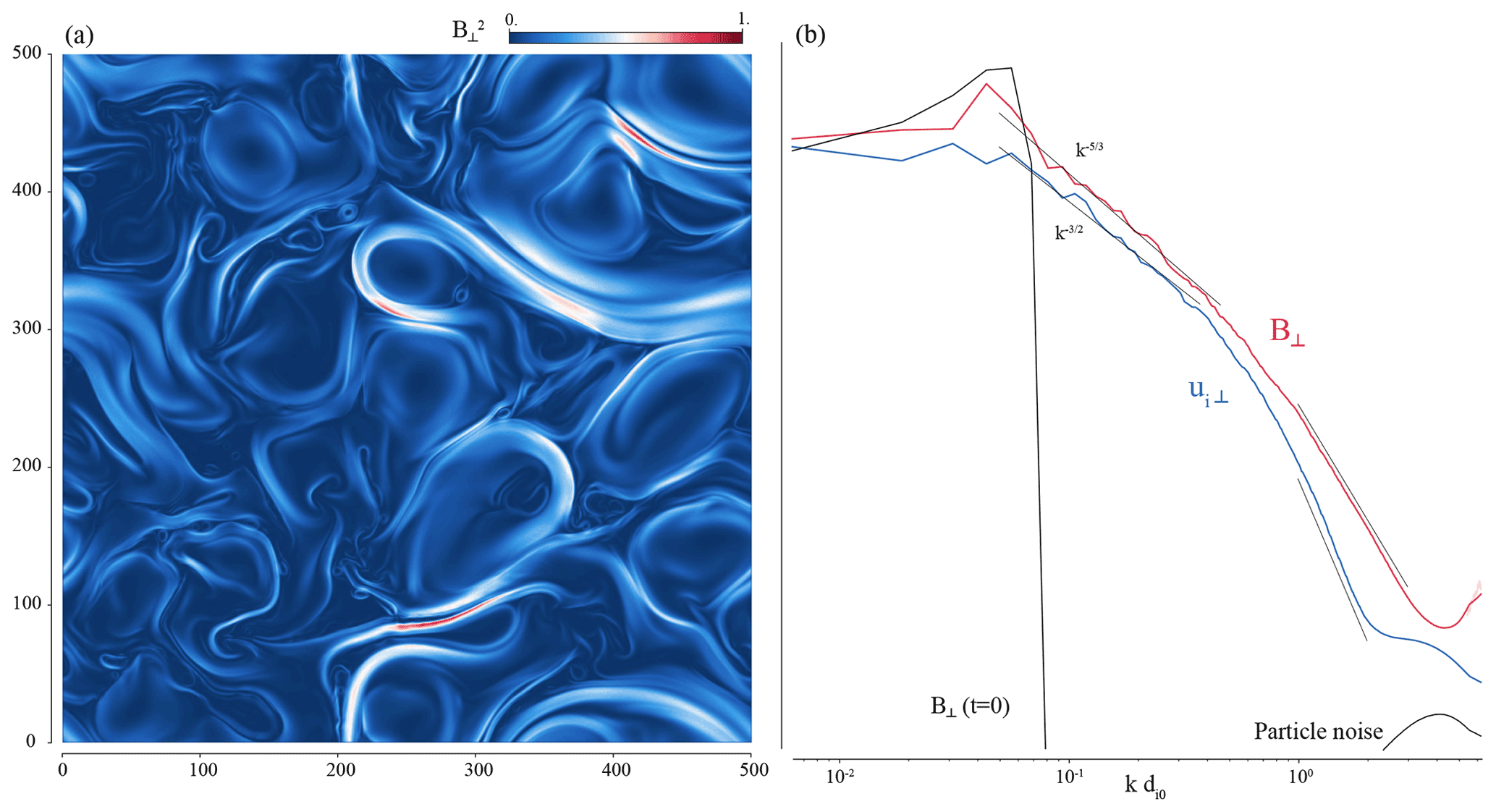
Figure 4Decaying turbulence at time 500 . (a) shows the squared in-plane (perpendicular) magnetic field amplitude, while (b) presents the omnidirectional power density spectra of the same perpendicular magnetic field as well as the perpendicular velocity field.
Menura has shown satisfactory results on plasma turbulence, over 3 orders of magnitude in wavenumbers. We now start the second phase of the simulation, resuming it at , corresponding to the snapshot studied in the previous section. We keep all parameters unchanged (including the polytropic index of 1 and the hyper-resistivity of ) but add an obstacle with a relative velocity with regard to the frame used in the first phase, evolving through this developed turbulence. Particles and fields are advanced with the exact same time and spatial resolutions as previously, so the interaction between this obstacle and the already-present turbulence is solved with the same self-consistency as in the first phase, with only one ingredient added: the obstacle.
5.1 A comet
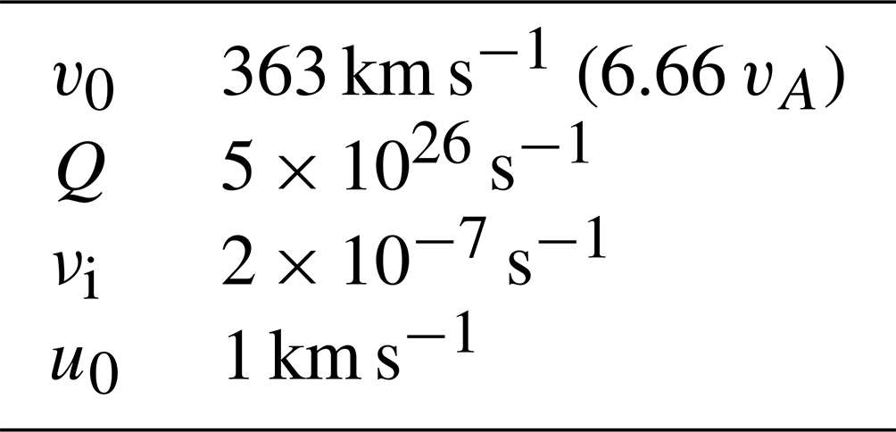
This obstacle is chosen here to be an intermediate activity comet, meaning that its neutral outgassing rate is typical of an icy nucleus at a distance of about 2 au from the Sun. A comet nucleus is from a few to a few tens of kilometres large, with a gravitational pull not strong enough to overcome the kinetic energy gained by the molecules during sublimation. Comprehensive knowledge on this particular orbital phase of comets has recently been generated by the European Rosetta mission, which orbited its host comet for 2 years (Glassmeier et al., 2007). The first and foremost interest of such an object for this study is the size of its plasma environment, which can be evaluated using the gyroradius of water ions in the solar wind at 2 au. The expected size of the interaction region is about 4 times this gyro-radius (Behar et al., 2018), and with the characteristic physical parameters of Table 2, the estimated size of the interaction region is 480 di0. In other words, the interaction region spans exactly over the range of spatial scales probed during the first phase of the simulation, including MHD and ion kinetic scales.
The second interest of a comet is its relatively simple numerical implementation. Considering the spatial resolution of the simulation, the solid nucleus can be neglected. By also neglecting the gravitational force on molecules as well as any intrinsic magnetic field, the obstacle is only made of cometary neutral particles being photo-ionised within the solar wind. Over the scales of interest for this study, the neutral atmosphere can be modelled by a radial density profile, and considering the coma to be optically thin, ions are injected in the system with a rate following the same profile. This is the Haser model (Haser, 1957), and simulating a comet over scales of hundreds of di0 only requires injecting cold cometary ions at each time step with the rate
with r the distance from the comet nucleus of negligible size, νi the ionisation rate of cometary neutral molecules, n0 the neutral cometary density, Q the neutral outgassing rate, and u0 the radial expansion speed of the neutral atmosphere.
One additional simplification is to limit the physico-chemistry of the cometary environment to photo-ionisation, thus neglecting charge exchanges between the solar wind and the coma, as well as electron impact ionisation. Both processes can significantly increase the ionisation of the neutral coma (Simon Wedlund et al., 2019). A global increase or a local change in the production profile is not expected to impact the initial main goal of the model, which is to simulate the turbulent nature of the solar wind during its interaction with an obstacle. We note however that the influence of upstream turbulence on the physico-chemistry of an obstacle is yet another promising prospect for the code.
5.2 Reference frame
The first phase of the simulation, the decaying turbulence phase, was done in the plasma frame, in which the average ion bulk velocity is 0. Classically, planetary plasma simulations are done in the planet reference frame: the obstacle is static and the wind flows through the simulation domain. In this case, a global plasma reference frame is most of the time not defined. In Menura, we have implemented the second phase of the simulation – the interaction phase – in the exact same frame as the first phase, which then corresponds to the plasma frame of the upstream solar wind, before interaction. In other words, the turbulent solar wind plasma is kept “static”, and the obstacle is moving through this plasma. The reason motivating this choice is to keep the turbulent solar wind “pristine”, by continuing its resolution over the exact same grid as in phase one. Another motivation for working in the solar wind reference frame is illustrated in Fig. 5, in which we compare the exact same simulation done in each frame, using a laminar upstream flow. If the macroscopic result remains unchanged between the two frames, we find strong small-scale numerical artifacts propagating upstream of the interaction in the comet reference frame, absent in the solar wind reference frame. Small-scale oscillations are common in hybrid PIC simulations and are usually filtered with either resistivity and/or hyper-resistivity, or with an ad hoc smoothing method. Note that none of these methods are used in the present example. We demonstrate here the role of the reference frame in the production of one type of small-scale oscillations and ensure that their influence over the spectral content of upstream turbulence is minimised, already without the implemented hyper-resistivity.
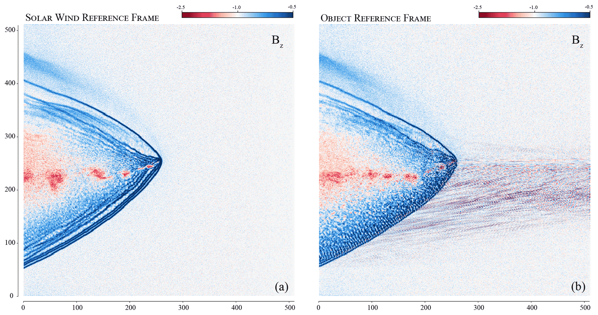
Figure 5The interaction between a comet and a laminar flow, in the object rest frame (a) and the upstream solar wind reference frame (b). The magnetic field amplitude is shown.
To summarise, by keeping the same reference frame during Step 1 and 2, the only effective difference between the two phases is the addition of sunward moving cometary macroparticles.
Another major advantage of working in the solar wind reference frame is the possibility to simulate magnetic field variations in all directions, including the relative plasma-object direction. For studying the interaction between co-rotating interaction regions and an object for instance, one needs to vary the direction of the magnetic field upstream of the object of interest. In the object reference frame, such a temporal variation of the magnetic field is frozen in the flow and advected downstream through the simulation domain by the convective electric field. Considering the ideal Ohm's law and Faraday's law , and considering a plasma flowing along the x axis , we get the time evolution of each magnetic field component as
The direct implication of this system is that any temporal variation we may force on the upstream Bx cannot have a self-consistent influence on the time evolution of the magnetic field elsewhere: only variations forced along magnetic field components perpendicular to the flow direction can be advected downstream, through this ideal frozen-in condition. In contrast, when working in the solar wind reference frame, we can impose spatial fluctuations of the magnetic field (equivalently temporal in the object frame) in all directions: in this frame these fluctuations are not being advected; it is rather the object itself moving through the fluctuations. This effectively removes the constraint on flow-aligned variation of the magnetic field, opening up promising possibilities for the simulation of various solar wind events, such as CIRs or sector boundary crossings.
5.3 Algorithm
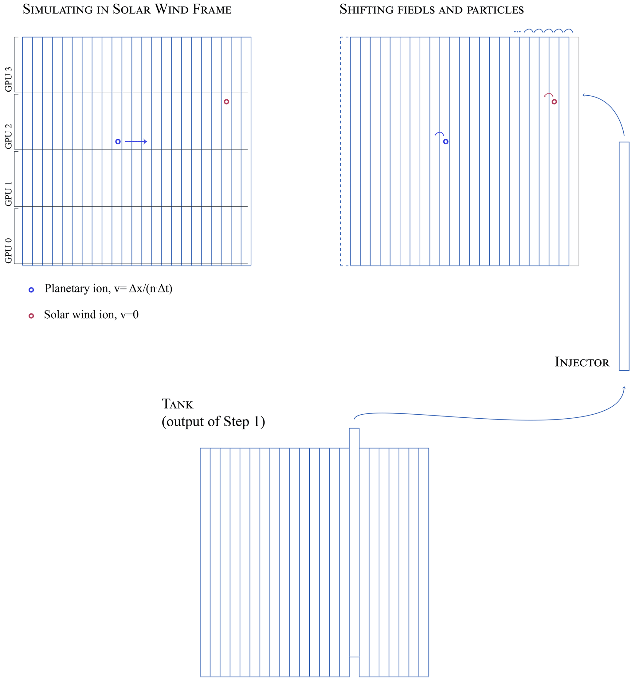
By working in the solar wind reference frame, the obstacle is moving within the simulation domain. Eventually, the obstacle would reach the boundaries of the box, before steady-state is reached. We therefore need to somehow keep the obstacle close to the centre of the simulation domain. This is done by shifting all particles and fields of nΔx every m iterations, , as illustrated in Fig. 6. Using integers, the shift of the field is simply a side-way copy of themselves without the need of any interpolation, and the shift of the particles is simply the subtraction of nΔx to their x coordinate. Field values as well as particles ending up downstream of the simulation domain are discarded.
This leaves only the injection boundary to be dealt with. There, we simply inject a slice of fields and particles picked from the output of Step 1, using the right slice index in order to inject the continuous turbulent solution, as shown in Fig. 6. These slices are nΔx wide.
With idx_it the index of the iteration, the algorithm illustrated in Fig. 6 is then as follows:
- –
Inject cometary ions according to qi(r) (cf. Eq. 11).
- –
Advance particles and fields (cf. Fig. 1).
- –
If
idx_it %m=0,- –
shift particles and fields of
-nΔx. - –
discard downstream values.
- –
inject upstream slice
idx_slicefrom Step 1 output. - –
increment
idx_slice.
- –
- –
Increment
idx_it.
This approach has one constraint, we cannot fine-tune the relative speed v0 between the wind and the obstacle, which has to be
in order for the obstacle to come back to its position every m iterations, and therefore not drift up- or downstream of the simulation domain.
5.4 CUDA and MPI implementation, performances
The computation done by Menura's solver (Fig. 1) is entirely executed on multiple GPUs (graphics processing units), written in C++ in conjunction with the CUDA programming model and the Message Passing Interface (MPI) standard, which allows splitting the problem and distributing it over multiple cards (i.e. processors). GPUs can run thousands of threads simultaneously and can therefore tremendously accelerate such applications. The first implementation of a hybrid-PIC model on such devices was done by Fatemi et al. (2017). However their still limited memory (up to 80 GB at the time of writing) is a clear constraint for large problems, especially for a turbulence simulation which requires a large range of spatial scales and a very large number of particles per grid node. The use of multiple cards becomes then unavoidable, and the communication between them is implemented using a CUDA-aware version of MPI. The division of the simulation domain in the current version of Menura is kept very simple, with equal size rectangular sub-domains distributed along the direction perpendicular to the motion of the obstacle: one sub-domain spans the entire domain along the x axis with its major dimension, as shown in Fig. 6. MPI communication is done for particles after each position advancement and for fields after each solution of Ohm's law and Faraday's law. But since the shift of fields and particles described in the previous section is done purely along the obstacle motion direction, no MPI communication is needed after the shifts, thanks to the orientation of the sub-domains.
Another limitation in using GPUs is the data transfer time between the CPU and the cards. In Menura, all variables are initialised on the CPU and are saved from the CPU. Data transfers are then unavoidable, before starting the main loop, and every time we want to save the current state of the variables. During Step 2 of the simulation, a copy of the outputs of Step 1 is needed, which effectively doubles the memory needed for Step 2. This copy is kept on the CPU (in the tank object) in order to make the most out of the GPU memory, in turn implying that more CPU–GPU communication is needed for this second step. Every time we inject a slice of fields and particles upstream of the domain, only this number of data is copied from the CPU to the GPUs, using the injector data structure as sketched in Fig. 6.
5.4.1 Profiling
For Step 1, the decaying turbulence ran 10 000 iterations, and four NVIDIA V100 GPUs were used with 16 GB memory each, corresponding to one complete node of the IDRIS cluster Jean Zay. A total of 2 billion particles (500 million per card) were initialised. The time for the solver on each card reached a bit more than 3 h, with a final total cost of about 13 h of computation time for this simulation, taking into account all four cards, and the variables initialisation and output. Step 2 was executed on larger V100 32 GB cards, providing much more room for the addition of 60 000 cometary macroparticles per iteration.
During Step 1, 87.3 % of the computation time was spent on moments mapping, i.e. steps 0 and 2 in the algorithm of Fig. 1, while respectively 2.7 % and 0.8 % were spent on advancing the particles velocity and position. The computation of Ohm's and Faraday's laws sums up to 0.5 %; 0.9 % was utilised for MPI communication of field variables, while only 0.08 % was dedicated for particles MPI communication, due to the limited particle transport happening in Step 1.
A total of 91 % of the total solver computation time is devoted to particles treatment, with 96 % of that part spent on particle moment mapping, which might seem a suspiciously large fraction. We note however that such a simulation is characterised by its large number of particles per node, 2000 in our case. A total of 99.6 % of the total allocated memory is devoted to particles. The time spent to map the particles on the grid is also remarkably larger than the time spent to update their velocity, despite both operations being based on the same interpolation scheme. However, during the mapping of the particle moments, thousands of particles need to increment the value at particular memory addresses (corresponding to macroparticle density and flux), whereas during the particle velocity advancement, thousands of particles only need to read the value of the same addresses (electric and magnetic field).
5.4.2 Scalability
An important part of performance testing for parallelised codes is the scalability of the parallelisation. When each parallel process is serial (i.e. one thread for one process), the strong and weak scaling of the code are classical performance tests, with theoretical laws available for comparison (respectively Amdahl's law and Gustafson's law). These laws cannot be directly adapted to the case of devices that already have a highly parallel structure, such as GPUs. We however can approach the same strong and weak scaling properties of the code to get some valuable insights on the performance of the Menura's MPI implementation.
Strong scaling refers to the speed-up (gain of computation time) obtained while simulating the same problem (same grid size and same number of particles per grid node) with a growing number of processes (the load thus decreasing on each GPU). The upper panel of Fig. 7 shows the speed-up obtained using from 1 to 25 processes (i.e. GPUs) solving the same problem: a homogeneous, fully periodic, 2D plasma box, with no initial disturbance, with total size 1000×1000 grid nodes and 1000 particles per grid node. V100 cards with 16 GB of RAM were used for all runs but one (see below). The speed-up is measured as . t denotes a computation time, counted from the start of the main algorithm loop to its end, thus excluding the variables' initialisation and output. Each run is completed five times, and the average value for each type of run is given in Fig. 7. tref is a reference computation time; tN is the computation time using N processes. The results are given in a log–log representation, to emphasise the behaviour of the code at low and large number of processes. To simplify the analysis and contrary to the usual approach followed for serial processes, tref is not chosen as tref=t1, but here as tref=t4 for the following reason. When using between 4 and 16 GPUs, we achieve the ideal scaling: when doubling the number of processes, we halve the computation time. In other words all lie along the straight line of slope (since tref is taken for four processes). Points for lower and higher number of processes diverge from this ideal scaling. For low numbers of processes, the reason for the relative slow-down is the memory usage of the cards. When dividing the problem between two cards, 87 % of their memory is used1, compared to the 47 % usage in the case of four processes. This reflects the fact that GPUs only possess a finite number of parallel threads, though this number surpasses 5000 for this precise hardware. In turn, when an operation needs more threads than available, the computation time is increased. On the opposite end of the test, for N>16, it is the irreducible operations, such as MPI communication or the kernels calls by the CPU, which become greater than the actual calculation time by the GPUs, and lead the speed-ups to diverge from the ideal linear evolution.
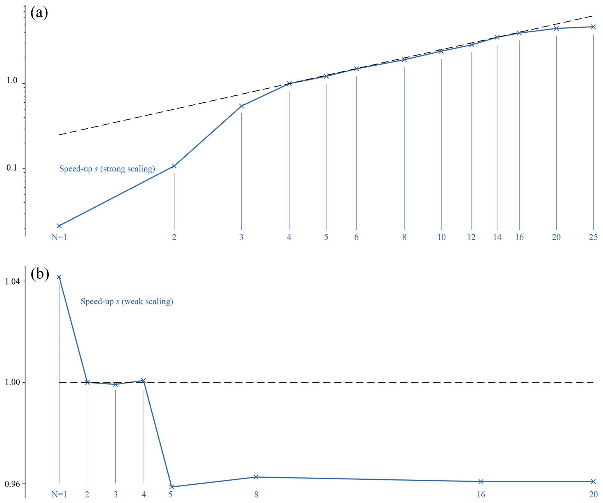
Figure 7Results for the strong (a) and weak (b) scaling properties of Menura. The strong scaling test consists of a simulation domain of a 1000×1000 grid with 1000 particles per grid node, divided into an increasing number of processes (i.e. GPUs). During the weak scaling test, the load on each GPU is kept constant (1000×125 grid, 1000 particles per node) and the number of processes is increased. The speed-up in both cases is defined as with here tref=t4.
The weak scaling of the code is measured by increasing the size of the problem while increasing the number of processes, keeping the same load on single processes. The results are given using the same definition of the speed-up, still using the run N=4 for reference. Each process now simulates a 1000×125 nodes domain with 1000 particles per node (thus corresponding to the previous N=8 run). Because of the much smaller differences in computation time, the scales are kept linear. As previously, s4 is defined as 1. The GPU memory usage is now 27 %, and the computation time is 260 s for the reference N=4. Using only one process results in a speed-up of 1.04; i.e. the runs completes about 4 % faster than the reference run. For , the computation time is equal within a second, resulting in a plateau of values around sN=1. For N>4, another plateau is reached with a speed-up of 0.96, now computing 4 % slower than the reference run, independently of the number of GPUs used. The interpretation of these three different values (1.04, 1.00 and 0.96) is straightforward. When running only one process, no MPI communication between processes is necessary, resulting in a faster run. Increasing the number of processes from two to four only involves the exact same amount of communication between neighbouring processes, not affecting the other communication, and the computation time is unchanged. From four to five (and more) processes, communication is now done between two or more computation nodes (with one compute node hosting four GPUs in Jean Zay cluster used here). Communicating data between cards within a same node is faster than between cards on different nodes, and therefore an observable slow-down happens at N=5. Increasing the number of nodes (from 8 cards to 16, then to 20) does not affect the computation time, for the same reason that increasing the number of cards within one node results in the same computation time.
These two tests exhibit a fine behaviour of Menura's MPI parallelisation, also showing that for this problem size, MPI communication does not cost more than 4 % to 8 % additional computation time, depending on the number of nodes used.
We now focus on the result of Step 2, in which cometary ions were steadily added to the turbulent plasma of Step 1, moving at a super-Alfvénic and super-sonic speed. Table 3 lists the physical parameters used for Step 2. After 4000 iterations, the total number of cometary macroparticles in the simulation domain reaches a constant average value: the comet is fully developed and has reached an average “steady” state. From this point, we simulate several full injection periods (1500 iterations), looping over the domain of the injection tank in Fig. 6. As an example, Fig. 8 displays the state of the system at iteration 6000, focusing here again on the perpendicular fluctuations of the magnetic field. This time the colour scale is logarithmic, since magnetic field fluctuations are spanning over a much wider range than previously. While being advected through a dense cometary atmosphere, the solar wind magnetic field piles up (augmentation of its amplitude because of the slowing down of the total plasma bulk velocity) and drapes (deformation of its field lines due to the differential pile-up around the density profile of the coma), as first theorised by Alfven (1957). This general result was always applied to the global, average magnetic field and was observed in situ at the various comets visited by space probes.
Without diving very deeply in the first results of Menura, we see that the pile-up and the draping of upstream perpendicular magnetic field fluctuations also has an important impact on the tail of the comet, with the creation of large amplitude magnetic field vortices of medium and small size. This phenomenon, together with a deeper exploration of the impact of solar wind turbulence on the physics of a comet, is gathered in a subsequent publication.

This publication introduces a new hybrid PIC plasma solver, Menura, that allows for the first time to investigate the impact of a turbulent plasma flow on an obstacle. For this purpose, a new two-step simulation approach has been developed which consist of, first, developing a turbulent plasma, and second, injecting it periodically in a box containing an obstacle. The model has been validated with respect to well-known fluid and kinetic plasma phenomena. Menura has also proven to provide the results expected at the output of this first step of the model – namely decaying magnetised plasma turbulence.
Until now, all planetary-science-oriented simulations have ignored all together the turbulent nature of the solar wind plasma flow, in terms of structures and in terms of energy. Menura has been designed to fulfil this deficiency, and it will now allow us to explore, for the first time, some fundamental questions that have remained open regarding the impact of the solar wind on different solar system objects, such as the following: what happens to turbulent magnetic field structures when the solar wind impacts on an obstacle such as a magnetosphere? How are the properties of a turbulent plasma flow reset as it crosses a shock, such as the solar wind crossing a planetary bow shock? How does the additional energy stored in the perpendicular magnetic and velocity field components impact the large-scale structures and dynamics of planetary magnetospheres?
On top of the study of the interaction between the turbulent solar wind and solar system obstacles, we are confident that the new modelling framework developed in this work, in particular its two-step approach, might as well be suitable for the study of energetic solar wind phenomena, namely co-rotating interaction regions and coronal mass ejections, which could be similarly simulated first in the absence of an obstacle, to then be used as inputs of a second step including obstacles.
In Menura's solver, all variables are normalised using the background magnetic field amplitude B0 and background density n0, or equivalently using the corresponding proton gyrofrequency ωci0 and Alfvén speed vA0. The background variable definitions are given in Table 1. Based on these definitions, one can derive the following main equations of the solver. A normalised variable is obtained by dividing this variable by its background value, , equivalently . We first consider Faraday's law, and using the background parameters definitions of Table 2:
with
In other words, Faraday's law expressed with normalised variables is unchanged compared to its SI definition. Ohm's law becomes
with
and
Concerning the gathering of particles moments,
with . For the solar wind proton, and one simply gets . stands for the shape factor, triangular in our case (in 2 spatial dimensions, one macroparticle affects the density and current of nine grid nodes, with linear weights).
Starting with the 2-dimensional Faraday's law (one can ignore the third component, which cannot take part in the divergence of the magnetic field since in 2 dimensions ),
discretised to
with the notation representing the discrete temporal and spatial derivatives. The five-point-stencil central finite difference discretisation of ∂yEz reads
The divergence of the magnetic field increment ΔB is then
The two consecutive finite differences on the electric field component can be expanded to
in which terms cancel each other two by two, resulting in a divergence-free magnetic field increment, div. It follows that only round-off errors will accumulate in the time evolution of div(B). The same argument is classically done for constrained transport schemes, which use staggered grids to ensure the same property, with the additional complexity of secondary variables for the electric and magnetic fields, and fields interpolation/averaging between cell centres and cell edges and corners. Tóth (2000) provides great insights on the constrained transport and finite central differences schemes, also showing that both conserve the magnetic field divergence.
The time evolution of the divergence of the magnetic field for the decaying turbulence run is shown in Fig. B1. We find that the variance of the divergence grows but remains smaller than 10−11, while the maximum value of the divergence (using its absolute value) remains lower than some , given an initial value of . This growth is due to accumulating round-off errors, over tens of thousand of magnetic field pushes. It was tested that for the exact same problem, increasing the number of time steps increases this accumulated error, despite a finer time resolution.
The total energy, despite a clear decrease over most of the simulation time, is bounded within +1 % and −4 %. An additional run was used, which does not include initial perturbation, i.e. a homogeneous plasma. This run shows a nearly perfect energy conservation, with departures of the order of 10−5 the total energy at initial time.

Figure B1Time evolution of the maximum of the divergence of the magnetic field (a) and of the total energy (b) for the decaying turbulence run.
The code is open-source and available at https://gitlab.com/etienne.behar/menura (also available on the Zenodo repository Behar, 2022), its documentation available at https://menura.readthedocs.io/en/latest/ (last access: 3 May 2022).
All data in the publication were produced and can be reproduced using Menura and its analysis tools. Jupyter notebooks are also provided (https://menura.readthedocs.io/en/latest/physical_tests.html, last access: 3 May 2022) as an example to reproduce the physical test analysis. The data set is not made available online.
EB is the developer of Menura and has executed all simulations shown in this publication and ran all analyses. SF and MH were significantly consulted during code development. All authors have designed the physical and technical tests and interpreted their results. All authors iterated together over the various versions of the publication.
The contact author has declared that neither they nor their co-authors have any competing interests.
Publisher’s note: Copernicus Publications remains neutral with regard to jurisdictional claims in published maps and institutional affiliations.
Etienne Behar thanks Matthew Kunz for the valuable discussion concerning constrained transport in the context of hybrid PIC codes.
Etienne Behar received support from the Swedish National Research Council (grant no. 2019-06289). This research was conducted using computational resources provided by the Swedish National Infrastructure for Computing (SNIC) (project nos. SNIC 2020/5-290 and SNIC 2021/22-24) at the High Performance Computing Center North (HPC2N), Umeå University, Sweden. This work was granted access to the HPC resources of IDRIS under the allocation 2021-AP010412309 made by GENCI. Work at LPC2E and Lagrange was partly funded by CNES. Shahab Fatemi received support from the Swedish Research Council (VR) (grant no. 2018-03454 and SNSA grant no. 115/18).
This paper was edited by Matina Gkioulidou and reviewed by two anonymous referees.
Alfven, H. t.: On the theory of comet tails, Tellus, 9, 92–96, 1957. a
Bagdonat, T. and Motschmann, U.: 3D Hybrid Simulation Code Using Curvilinear Coordinates, J. Comput. Phys., 183, 470–485, https://doi.org/10.1006/jcph.2002.7203, 2002. a, b
Behar, E.: Menura, Zenodo [code], https://doi.org/10.5281/zenodo.6517018, 2022 (code available at: https://gitlab.com/etienne.behar/menura, last access: 3 May 2022). a
Behar, E., Tabone, B., Saillenfest, M., Henri, P., Deca, J., Lindkvist, J., Holmström, M., and Nilsson, H.: Solar wind dynamics around a comet-A 2D semi-analytical kinetic model, Astron. Astrophys., 620, A35, https://doi.org/10.1051/0004-6361/201832736, 2018. a
Boldyrev, S., Perez, J. C., Borovsky, J. E., and Podesta, J. J.: Spectral scaling laws in magnetohydrodynamic turbulence simulations and in the solar wind, Astrophys. J., 741, L19, https://doi.org/10.1088/2041-8205/741/1/l19, 2011. a
Boris, J. P.: Relativistic plasma simulation-optimization of a hybrid code, in: Proc. Fourth Conf. Num. Sim. Plasmas, 3–67, https://apps.dtic.mil/sti/citations/ADA023511 (last access: 3 May 2022), 1970. a
Borovsky, J. E. and Funsten, H. O.: MHD turbulence in the Earth's plasma sheet: Dynamics, dissipation, and driving, J. Geophys. Res.-Space, 108, A7, https://doi.org/10.1029/2002JA009625, 2003. a
Bruno, R. and Carbone, V.: Turbulence in the solar wind, vol. 928, Springer, 2013. a, b
Chapman, S. C. and Hnat, B.: Quantifying scaling in the velocity field of the anisotropic turbulent solar wind, Geophys. Res. Lett., 34, L17103, https://doi.org/10.1029/2007GL030518, 2007. a
D’Amicis, R., Telloni, D., and Bruno, R.: The Effect of Solar-Wind Turbulence on Magnetospheric Activity, Front. Phys., 8, 541, https://doi.org/10.3389/fphy.2020.604857, 2020. a
Edberg, N. J., Alho, M., André, M., Andrews, D. J., Behar, E., Burch, J., Carr, C., Cupido, E., Engelhardt, I., and Eriksson, A. I.: CME impact on comet 67P/Churyumov-Gerasimenko, Mon. Not. R. Astron. Soc., 462, S45–S56, 2016. a
Exner, W., Heyner, D., Liuzzo, L., Motschmann, U., Shiota, D., Kusano, K., and Shibayama, T.: Coronal mass ejection hits mercury: A.I.K.E.F. hybrid-code results compared to MESSENGER data, Planet. Space Sci., 153, 89–99, https://doi.org/10.1016/j.pss.2017.12.016, 2018. a
Fatemi, S., Poppe, A. R., Delory, G. T., and Farrell, W. M.: AMITIS: A 3D GPU-Based Hybrid-PIC Model for Space and Plasma Physics, J. Phys.-Conf. Ser., 837, 012017, https://doi.org/10.1088/1742-6596/837/1/012017, 2017. a
Franci, L., Landi, S., Matteini, L., Verdini, A., and Hellinger, P.: High-resolution hybrid simulations of kinetic plasma turbulence at proton scales, Astrophys. J., 812, 21, https://doi.org/10.1088/0004-637x/812/1/21, 2015. a, b, c, d
Glassmeier, K.-H., Boehnhardt, H., Koschny, D., Kührt, E., and Richter, I.: The Rosetta mission: flying towards the origin of the solar system, Space Sci. Rev., 128, 1–21, 2007. a
Goldreich, P. and Sridhar, S.: Magnetohydrodynamic Turbulence Revisited, Astrophys. J., 485, 680–688, https://doi.org/10.1086/304442, 1997. a
Gombosi, T., Powell, K., De Zeeuw, D., Clauer, C., Hansen, K., Manchester, W., Ridley, A., Roussev, I., Sokolov, I., Stout, Q., and Toth, G.: Solution-adaptive magnetohydrodynamics for space plasmas: Sun-to-Earth simulations, Comput. Sci. Eng., 6, 14–35, https://doi.org/10.1109/MCISE.2004.1267603, 2004. a
Guio, P. and Pécseli, H. L.: The Impact of Turbulence on the Ionosphere and Magnetosphere, Front. Astron. Space Sci., 7, 107, https://doi.org/10.3389/fspas.2020.573746, 2021. a
Hajra, R., Henri, P., Myllys, M., Héritier, K. L., Galand, M., Simon Wedlund, C., Breuillard, H., Behar, E., Edberg, N. J. T., Goetz, C., Nilsson, H., Eriksson, A. I., Goldstein, R., Tsurutani, B. T., Moré, J., Vallières, X., and Wattieaux, G.: Cometary plasma response to interplanetary corotating interaction regions during 2016 June–September: a quantitative study by the Rosetta Plasma Consortium, Mon. Not. R. Astron. Soc., 480, 4544–4556, https://doi.org/10.1093/mnras/sty2166, 2018. a
Haser, L.: Distribution d'intensité dans la tête d'une comète, Bulletin de la Societe Royale des Sciences de Liege, 43, 740–750, 1957. a
Holmström, M.: Handling vacuum regions in a hybrid plasma solver, 2013. a
Kiyani, K. H., Osman, K. T., and Chapman, S. C.: Dissipation and heating in solar wind turbulence: from the macro to the micro and back again, Philos. T. R. Soc. A, 373, 20140155, https://doi.org/10.1098/rsta.2014.0155, 2015. a
Kraichnan, R. H.: Inertial-Range Spectrum of Hydromagnetic Turbulence, Phys. Fluid., 8, 1385–1387, https://doi.org/10.1063/1.1761412, 1965. a
Luhmann, J. G., Fedorov, A., Barabash, S., Carlsson, E., Futaana, Y., Zhang, T. L., Russell, C. T., Lyon, J. G., Ledvina, S. A., and Brain, D. A.: Venus Express observations of atmospheric oxygen escape during the passage of several coronal mass ejections, J. Geophys. Res.-Planet., 113, https://doi.org/10.1029/2008JE003092, 2008. a
Markidis, S., Lapenta, G., and Rizwan-uddin: Multi-scale simulations of plasma with iPIC3D, Mathemat. Comput. Simul., 80, 1509–1519, https://doi.org/10.1016/j.matcom.2009.08.038, 2010. a
Maron, J. L., Low, M.-M. M., and Oishi, J. S.: A Constrained-Transport Magnetohydrodynamics Algorithm with Near-Spectral Resolution, Astrophys. J., 677, 520–529, https://doi.org/10.1086/525011, 2008. a
Matthews, A. P.: Current Advance Method and Cyclic Leapfrog for 2D Multispecies Hybrid Plasma Simulations, J. Comput. Phys., 112, 102–116, https://doi.org/10.1006/jcph.1994.1084, 1994. a, b
Podesta, J. J., Roberts, D. A., and Goldstein, M. L.: Spectral Exponents of Kinetic and Magnetic Energy Spectra in Solar Wind Turbulence, Astrophys. J., 664, 543–548, https://doi.org/10.1086/519211, 2007. a
Rakhmanova, L., Riazantseva, M., and Zastenker, G.: Plasma and Magnetic Field Turbulence in the Earth’s Magnetosheath at Ion Scales, Front. Astron. Space Sci., 7, 115, https://doi.org/10.3389/fspas.2020.616635, 2021. a
Ramstad, R., Barabash, S., Futaana, Y., Yamauchi, M., Nilsson, H., and Holmström, M.: Mars Under Primordial Solar Wind Conditions: Mars Express Observations of the Strongest CME Detected at Mars Under Solar Cycle #24 and its Impact on Atmospheric Ion Escape, Geophys. Res. Lett., 44, 10805–10811, https://doi.org/10.1002/2017GL075446, 2017. a
Rönnmark, K.: Waves in homogeneous, anisotropic multicomponent plasmas (WHAMP), https://inis.iaea.org/search/search.aspx?orig_q=RN:14744092 (last access: 3 May 2022), 1982. a
Sahraoui, F., Goldstein, M. L., Belmont, G., Canu, P., and Rezeau, L.: Three Dimensional Anisotropic k Spectra of Turbulence at Subproton Scales in the Solar Wind, Phys. Rev. Lett., 105, 131101, https://doi.org/10.1103/PhysRevLett.105.131101, 2010. a
Saur, J.: Turbulence in the Magnetospheres of the Outer Planets, Front. Astron. Space Sci., 8, 56, https://doi.org/10.3389/fspas.2021.624602, 2021. a
Simon Wedlund, C., Behar, E., Nilsson, H., Alho, M., Kallio, E., Gunell, H., Bodewits, D., Heritier, K., Galand, M., Beth, A., Rubin, M., Altwegg, K., Volwerk, M., Gronoff, G., and Hoekstra, R.: Solar wind charge exchange in cometary atmospheres – III. Results from the Rosetta mission to comet 67P/Churyumov-Gerasimenko, Astron. Astrophys., 630, A37, https://doi.org/10.1051/0004-6361/201834881, 2019. a
Tóth, G.: The ∇·B=0 Constraint in Shock-Capturing Magnetohydrodynamics Codes, J. Comput. Phys., 161, 605–652, https://doi.org/10.1006/jcph.2000.6519, 2000. a, b
Tskhakaya, D.: The Particle-in-Cell Method, Springer Berlin Heidelberg, Berlin, Heidelberg, 161–189, https://doi.org/10.1007/978-3-540-74686-7_6, 2008. a, b
Tsurutani, B. T. and Gonzalez, W. D.: The cause of high-intensity long-duration continuous AE activity (HILDCAAs): Interplanetary Alfvén wave trains, Planet. Space Sci., 35, 405–412, https://doi.org/10.1016/0032-0633(87)90097-3, 1987. a
Valentini, F., Trávníček, P., Califano, F., Hellinger, P., and Mangeney, A.: A hybrid-Vlasov model based on the current advance method for the simulation of collisionless magnetized plasma, J. Comput. Phys., 225, 753–770, https://doi.org/10.1016/j.jcp.2007.01.001, 2007. a, b
One larger 32 GB card was used for the case of N=1.
- Abstract
- Introduction
- The solver
- Physical tests
- Step 1: decaying turbulence
- Step 2: obstacle
- First result
- Conclusions
- Appendix A: Normalised equations
- Appendix B: ∇⋅B and total energy
- Code availability
- Data availability
- Author contributions
- Competing interests
- Disclaimer
- Acknowledgements
- Financial support
- Review statement
- References