the Creative Commons Attribution 4.0 License.
the Creative Commons Attribution 4.0 License.
 | 06 May 2022
Terrestrial exospheric dayside H-density profile at 3–15 RE from UVIS/HDAC and TWINS Lyman-α data combined
Jochen H. Zoennchen
Hyunju K. Connor
Jaewoong Jung
Uwe Nass
Hans J. Fahr
Terrestrial ecliptic dayside observations of the exospheric Lyman-α column intensity between 3–15 Earth radii (RE) by UVIS/HDAC (UVIS – ultraviolet imaging spectrograph; HDAC – hydrogen-deuterium absorption cell) Lyman-α photometer at CASSINI have been analyzed to derive the neutral exospheric H-density profile at the Earth's ecliptic dayside in this radial range. The data were measured during CASSINI's swing-by maneuver at the Earth on 18 August 1999 and are published by Werner et al. (2004). In this study the dayside HDAC Lyman-α observations published by Werner et al. (2004) are compared to calculated Lyman-α intensities based on the 3D H-density model derived from TWINS (Two Wide-angle Imaging Neutral-atom Spectrometers) Lyman-α observations between 2008–2010 (Zoennchen et al., 2015). It was found that both Lyman-α profiles show a very similar radial dependence in particular between 3–8 RE. Between 3.0–5.5 RE impact distance Lyman-α observations of both TWINS and UVIS/HDAC exist at the ecliptic dayside. In this overlapping region the cross-calibration of the HDAC profile against the calculated TWINS profile was done, assuming that the exosphere there was similar for both due to comparable space weather conditions. As a result of the cross-calibration the conversion factor between counts per second and rayleigh, fc=3.285 counts s−1 R−1, is determined for these HDAC observations.
Using this factor the radial H-density profile for the Earth's ecliptic dayside was derived from the UVIS/HDAC observations, which constrained the neutral H density there at 10 RE to a value of 35 cm−3. Furthermore, a faster radial H-density decrease was found at distances above 8 RE () compared to the lower distances of 3–7 RE (). This increased loss of neutral H above 8 RE might indicate a higher rate of H ionization in the vicinity of the magnetopause at 9–11 RE (near subsolar point) and beyond, because of increasing charge exchange interactions of exospheric H atoms with solar wind ions outside the magnetosphere.
- Article
(472 KB) - Full-text XML
- BibTeX
- EndNote


The Earth's exosphere is the outermost layer of our atmosphere that ranges from ≈ 500 km altitude to beyond the Moon's orbit (Baliukin et al., 2019). Atomic hydrogen atom (H) becomes a dominant species above an altitude of ≈ 1500 km. The exosphere gains and loses hydrogen atoms as a result of the Sun–solar-wind–magnetosphere–upper-atmosphere interaction. Study of the exospheric density distribution and its response to dynamic space environments is key to understand the past, present, and future of the Earth's atmosphere and to infer the evolution of other planetary atmospheres.
The typical geocorona emission, i.e., solar Lyman-α photons resonantly scattered by hydrogen atoms, has been a widely used dataset to derive a terrestrial exospheric neutral H density. Several spacecraft missions like Thermosphere–Ionosphere–Mesosphere Energetics and Dynamics (TIMED; Kusnierkiewicz, 1997), Two Wide-angle Imaging Neutral-atom Spectrometers (TWINS; Goldstein and McComas, 2018), and Solar and Heliospheric Observatory (SOHO; Domingo et al., 1995) have observed the geocorona from various vantage points, covering an optically thick, near-Earth exosphere below ≈ 3 RE geocentric distance (e.g., Qin and Waldrop, 2016; Qin et al., 2017; Waldrop and Paxton, 2013) to an optically thin, far distant exosphere on top (e.g., Bailey and Gruntman, 2011; Cucho-Padin and Waldrop, 2019; Zoennchen et al., 2011, 2013). The exospheric density changes over various timescales such as solar cycle (Waldrop and Paxton, 2013; Zoennchen et al., 2015; Baliukin et al., 2019), solar rotation (Zoennchen et al., 2015), and geomagnetic storms (Bailey and Gruntmann, 2013; Cucho-Padin and Waldrop, 2019; Qin et al., 2017; Zoennchen et al., 2017). This implies an active response of our exosphere to a dynamic space environment through physical processes like thermal expansion, photoionization, and charge exchanges as suggested in the previous theoretical studies (Chamberlain, 1963; Bishop, 1985; Hodges, 1994, and references therein). Also the possible contribution of non-thermal hydrogen to the exosphere is discussed (e.g., Qin and Waldrop, 2016; Fahr et al., 2018).
Recently, exospheric neutral H density at the 10 RE subsolar location became particularly interesting due to two upcoming missions: the NASA Lunar Environment heliospheric X-ray Imager (LEXI; http://sites.bu.edu/lexi, last access: 1 May 2021) and the joint ESA–China mission Solar wind–Magnetosphere–Ionosphere Link Explorer (SMILE; Branduardi-Raymont et al., 2018), with expected launches in 2023 and 2024, respectively. Soft X-ray imagers on these spacecrafts will observe motion of the Earth's magnetosheath and cusps in soft X-rays with a primary goal of understanding the magnetopause reconnection modes under various solar wind conditions. Soft X-rays are emitted due to interaction between the exospheric neutrals and the highly charged solar wind ions like O7+ and O8+ (Sibeck et al., 2018; Connor et al., 2021). Neutral density is a key parameter that controls the strength of soft X-ray signals. Denser hydrogen areas increase their interaction probability with solar wind ions and thus enhance soft X-ray signals, which is preferable for the LEXI and SMILE missions.
The dayside geocoronal observations above 8 RE radial distance are very rare. For estimating an exospheric density at the 10 RE subsolar location, Connor and Carter (2019) and Fuselier et al. (2010, 2020) used alternative datasets: the soft X-ray observations from the X-ray Multi-Mirror Mission astrophysics mission (XMM-Newton; Jansen et al., 2001) and the energetic neutral atom (ENA) observations from the Interstellar Boundary Explorer (IBEX; McComas et al., 2009), respectively. Their density estimates at 10 RE show a large discrepancy, ranging from 4 to 59 cm−3 with a lower limit from the IBEX observations and an upper limit from the XMM observations. However, these studies analyzed only a handful of events. Additionally, inherent difference of the soft X-ray and ENA datasets leads to different density extraction techniques, possibly contributing to the neutral density discrepancy. To understand the true nature of this outer dayside exosphere, more statistical and cumulative approaches with various datasets are needed.
We estimate a dayside exospheric density in a radial distance of 3–15 RE using rare dayside geocorona observations obtained from the CASSINI UVIS/HDAC (UVIS – ultraviolet imaging spectrograph; HDAC – hydrogen-deuterium absorption cell) Lyman-α instrument on 18 August 1999. This paper is structured as follows. Section 2 introduces the CASSINI Lyman-α observations on 18 August 1999. Section 3 discusses the solar conditions and interplanetary Lyman-α background during the observation period. Section 4 explains our density extraction approach. Section 5 estimates the conversion factor of the CASSINI UVIS/HDAC geocorona count rates to rayleigh, and Sect. 6 derives the dayside exospheric density profiles from the converted geocoronal emission in rayleigh. Finally, Sect. 7 discusses and concludes our results.
On its way to Saturn the CASSINI spacecraft performed a swing-by maneuver at the Earth on 18 August 1999. The UVIS/HDAC Lyman-α instrument (field of view ≈ 3∘) was switched on before and then measured continuously Lyman-α intensities during the maneuver. When approaching the Earth, the measured Lyman-α intensities were increasingly dominated by scattered Lyman-α emission from neutral H atoms of the terrestrial exosphere. The intensity profile in counts per second (averaged over a 1 min interval) from UVIS/HDAC is a rare observation of the exospheric dayside Lyman-α emission near the Earth–Sun line up to 15 RE geocentric distance. It is a nearly perfect scan within the ecliptic plane during ≈ 1.5 h and therefore nearly free from latitudinal and temporal variations. The profile was published by Werner et al. (2004) and is shown in Fig. 2 of their paper. From each measurement, they had subtracted 4500 counts s−1 as correction for their estimate of the interplanetary background intensity. For the geocentric distances of 3–15 RE, this corrected profile can be numerically approximated by the following fit function:
with the geocentric distance r in RE. The fitted radial intensity function from Eq. (1) is shown in Fig. 1, which approximates the profile very well in Werner et al. (2004, shown there in Fig. 2). Values from Eq. (1) need to be re-added with 4500 counts s−1 in order to retrieve the uncorrected intensities originally measured by UVIS/HDAC:
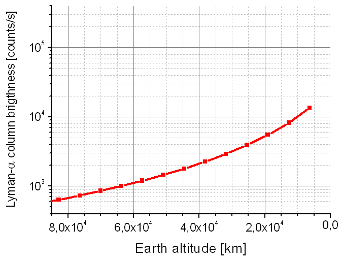
Figure 1Numerical approximation by Eq. (1) of the dayside exospheric UVIS/HDAC Lyman-α intensity profile [counts s−1] published by Werner et al. (2004, shown there in Fig. 2).
The observational geometry (spacecraft position and viewing direction of UVIS/HDAC) during the swing-by was also adopted from Werner et al. (2004): on the Earth dayside CASSINI moved within the ecliptic plane towards Earth. CASSINI's dayside trajectory as shown in Werner et al. (2004 – see Fig. 1 there) is nearly linear within 3–15 RE. It can be numerically approximated as a radial function of the GSE (Geocentric Solar Ecliptic System) longitude:
with the geocentric distance r in RE. Following Werner et al. (2004) in this trajectory, segment the line of sight (LOS) of UVIS/HDAC pointed towards the positive GSE y axis away from Earth. More UVIS/HDAC instrumental facts can be found in the “UVIS User's Guide” provided by the NASA PDS website (see: https://pds-atmospheres.nmsu.edu/data_and_services/atmospheres_data/Cassini/inst-uvis.html, last access: 1 November 2021)
The total solar Lyman-α flux and the solar F10.7 cm radio flux are important indicators of the solar activity. The solar Lyman-α flux can vary from 3.5 (solar minimum) to 6.5 (solar maximum) × 1011 photons cm−2 s−1. The solar F10.7 cm radio flux can vary from below 50 (solar minimum) to above 300 sfu (solar flux units; solar maximum). On the swing-by date, 18 August 1999, the value of the total solar Lyman-α flux was 4.52 – a bit higher than the value of ≈ 3.5 during the TWINS LAD observations in 2008 and 2010. It has been measured by TIMED SEE and SORCE SOLSTICE calibrated to UARS SOLSTICE level (Woods et al., 2000) (provided by LASP, Laboratory For Atmospheric And Space Physics, University of Colorado Boulder). With the function given by Emerich et al. (2005), the line-center solar Lyman-α flux was calculated from this total solar Lyman-α flux for the derivation of the g-factor as used in Eq. (4).
The solar activity level as indicated by the solar F10.7 cm radio flux starts to increase in summer 1999 from the low values of the solar minimum until 1998. With 130 as the F10.7 cm value during the UVIS/HDAC observations, it is also a bit higher compared to ≈ 80 during the TWINS LAD observations in 2008 and 2010.
When flying at the Earth dayside between 3–15 RE, the UVIS/HDAC LOS pointed to a region with interplanetary Lyman-α background of about 1400 R. This value was taken from the SOHO-SWAN all-sky map of the Lyman-α background on 17 August 1999 (SOHO-SWAN images provided via web by LATMOS-IPSL, Université Versailles St-Quentin, CNRS, France: http://swan.projet.latmos.ipsl.fr/images/, last access: 9 May 2021).
During the swing-by at the Earth, the UVIS/HDAC instrument measured Lyman-α radiation resonantly backscattered from neutral hydrogen of the terrestrial exosphere and also from the interplanetary medium. Due to their low velocities, the contributing H atoms can be considered “cold”. Therefore, this backscattered radiation contains wavelengths with a relatively narrow bandwidth around the Lyman-α line center. The sole contribution of the interplanetary hydrogen was quantified by the value taken from SOHO-SWAN as described in the previous section.
Within the exosphere the optical depth turns out to be lower than 1 at geocentric distances >3 RE, which allows for the assumption of single scattering. Under this assumption for a particular solar Lyman-α radiation (manifested in the g-factor), the exospheric H density N(S) along a line of sight S produces a Lyman-α scatter intensity I in rayleigh:
with n(S) being the local H density, ϵ(S) being the local correction term for geocoronal self-absorption or re-emission, and Ip(α(S)) being the local intensity correction for the angular dependence of the scattering.
In addition to the solar radiation, the dayside Lyman-α observations above 3 RE analyzed in this study are illuminated by a secondary Lyman-α radiation from lower atmospheric shells of the Earth: at the dayside lower, optically thick exospheric shells are face-on illuminated by the Sun. The re-emission created there acts as a secondary source of Lyman-α besides the Sun. The relative effect increases with decreasing geocentric distance. With the ϵ(S) term in Eq. (4), the Lyman-α intensity profile can be corrected from re-emission of solar Lyman-α from lower atmospheric shells of the Earth. The applied method in this study considered correction terms and the used map (shown in Fig. 2); a detailed described is given in Zoennchen et al. (2015).
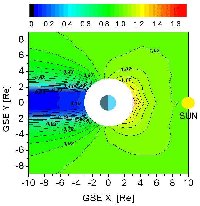
Figure 2Local ratio of the local Lyman-α illumination (influenced by multiple scattering effects) and the original solar illumination within the ecliptic plane calculated with a multiple scattering Monte Carlo model (Zoennchen et al., 2015).
With usage of a given H-density distribution, the Lyman-α column brightness can be calculated for any LOS and observing position within the optically thin regime based on the integral in Eq. (4). The calculated values ([R]) can be converted into their observable intensities ([counts s−1]) using a single instrumental factor ([counts s−1 R−1]) – further referred to as conversion factor fc.
In this study, two H-density models are used for comparison with UVIS/HDAC: the exospheric –density model derived from TWINS Lyman-α observations from 2008 and 2010 (Zoennchen et al., 2015 – with parameters from Table 1 there) and a radial symmetric model as introduced by Chamberlain (1963) and frequently used, for example, by Rairden et al. (1986), Fuselier et al. (2010, 2020), or Connor and Carter (2019):
with the geocentric distance r in RE. The H density at 10 RE subsolar point (n0) is set at 40 cm−3, which is within the reported range of Connor and Carter (2019) that derived n0 from the XMM soft X-ray emission.
The used TWINS model is an empirical 3D model of the neutral exospheric H density with validity range of 3–8 RE. It is based on the inversion of Lyman-α LOS observations of the TWINS satellites from the solar minimum in 2008 and 2010.
The other density model was introduced by Chamberlain (1963) as an analytical approach that is based on three different H-atom populations in the exosphere (ballistic, satellite, and escaping), with an initial Maxwellian distribution function at the exobase and the assumption of constant distribution functions on H-atom trajectories (Liouville's theorem). The theoretical fundamentals are very well summarized in Beth et al. (2016).
The comparison of the calculated profiles with the UVIS/HDAC profile was made for two reasons: first, to compare their radial dependency and second to derive the conversion factor fc of UVIS/HDAC by cross-calibrating it against the calculated profile from the TWINS H-density model in the radial range 3.0–5.5 RE (overlapping range). Dayside Lyman-α observations with impact distances inside this overlapping range are available by both UVIS/HDAC and TWINS. This method for evaluation of fc assumes that the TWINS H-density model from 2008 and 2010 also matches the exospheric H-density distribution on 18 August 1999 due to comparable space weather conditions. Both the used TWINS and UVIS/HDAC observations were measured during quiet geomagnetic conditions (minimum Dst index nT; provided by the website of the World Data Center for Geomagnetism, Kyoto) and low solar activity (indicated by solar F10.7 cm radio flux ≤ 130 sfu).
Nevertheless, it is known from other studies that the terrestrial exosphere shows H-density variations of about 10 %–20 % caused by geomagnetic storms (i.e. Bailey and Gruntman, 2013; Zoennchen et al., 2017; Cucho-Padin and Waldrop, 2019). Therefore, we expect an error in the conversion factor by this variations up to 20 %.
The observed dayside Lyman-α profile (column intensity) by UVIS/HDAC (approximated in Eq. 2) was compared to the calculated Lyman-α profiles (column brightness) from two exospheric H-density models described in the previous section. CASSINI's trajectory at the dayside between 3–15 RE, the LOS of HDAC, the interplanetary background, and the solar conditions of the swing-by day 18 August 1999 were considered by the calculation.
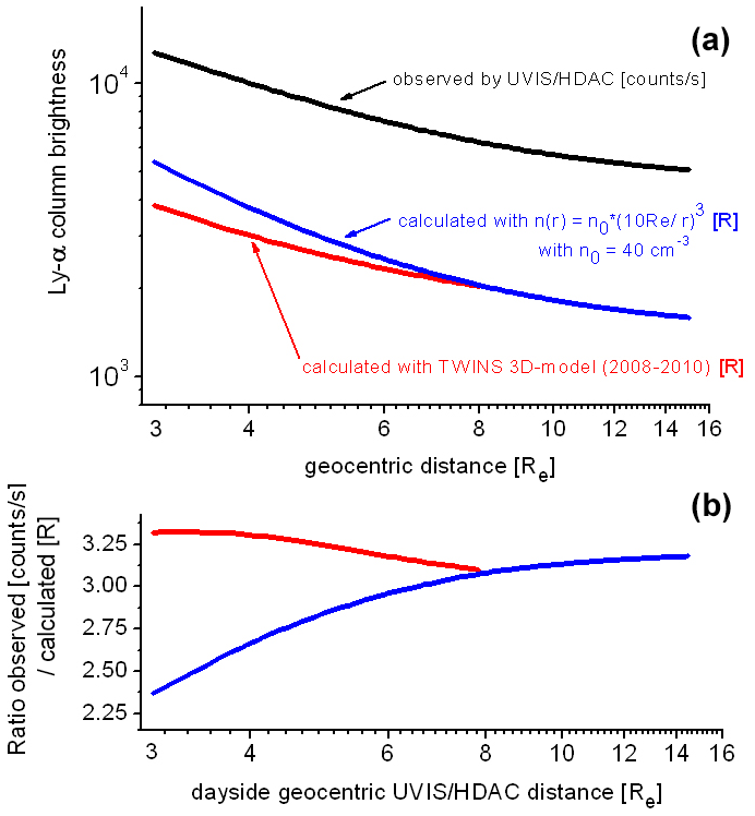
Figure 3(a) Observed, uncorrected Lyman-α profile by UVIS/HDAC [counts s−1] from Eq. (2) (black line) and the calculated column brightness profiles based on the TWINS 3D H-density model (red line) and the model (blue line), both including background and in rayleigh. (b) Ratios between the UVIS/HDAC observed and calculated profiles, with the TWINS H-density model (red line) and with the model (blue line).
Figure 3a shows the uncorrected observed Lyman-α profile by UVIS/HDAC from Eq. (2) in counts per second (black line) together with the calculated column brightness profiles in rayleigh based on the TWINS 3D H-density model inside its validity range of 3–8 RE (represented by the red line) and the model (blue line) – all including interplanetary Lyman-α background. It is obvious from that figure that between 3–8 RE the radial dependence of the calculated profile using the TWINS 3D H-density model corresponds well to the UVIS/HDAC observed profile. The radial dependency of the profile (blue line) deviates from the HDAC profile in this particular range.
Figure 3b shows the ratios of the observed and the calculated profiles: in the overlapping range (3.0–5.5 RE) the averaged ratio between the UVIS/HDAC observations and the TWINS 3D H-density model (red line) is nearly constant with only slight variations between −2.1 % and +1.2 %. It is equivalent to the averaged conversion factor and was found to be fc=3.285 counts s−1 R−1.
For the model (blue line), the ratio shows significant deviations from a constant value for lower radial distances < 8 RE. But for distances above 9 RE the profile of this model also turned into a nearly constant ratio compared to the UVIS/HDAC data (average = 3.145 counts s−1 R−1).
Besides the cross-calibration method, there is another independent way to approximate fc: Werner et al. (2004) estimated the interplanetary Lyman-α background in the UVIS/HDAC observations with 4500 counts s−1. To be not contaminated with exospheric emission, this value had to be measured far enough outside the exosphere. The interplanetary Lyman-α radiation is also created by resonant backscattering and is therefore comparable in its physical properties to exospheric emission. Using the Lyman-α background emission value from SOHO-SWAN in rayleigh for the UVIS/HDAC LOS, the conversion factor fc can be approximated on this separate way:
The two results for fc, with fc=3.285 from the profile comparison using the TWINS H-density model and fc=3.215 from the background estimation by Werner et al. (2004), are relatively close together.
We applied the determined conversion factor fc=3.285 counts s−1 R−1 to convert the observed dayside Lyman-α profile by UVIS/HDAC from intensities [counts s−1] into column brightness [R] between 3–15 RE. Inverse usage of Eq. (4) with known column brightnesses I(S) allows us to fit the H-density profile. The H-density profile inverted from the UVIS/HDAC observations was fitted into the radial symmetric function:
with geocentric distance r in RE. Figure 4 shows the fitted H-density profile (black squares). From the nH(r) profile, the UVIS/HDAC observations can be calculated very precisely over the entire radial range 3–15 RE within ±2 % error.
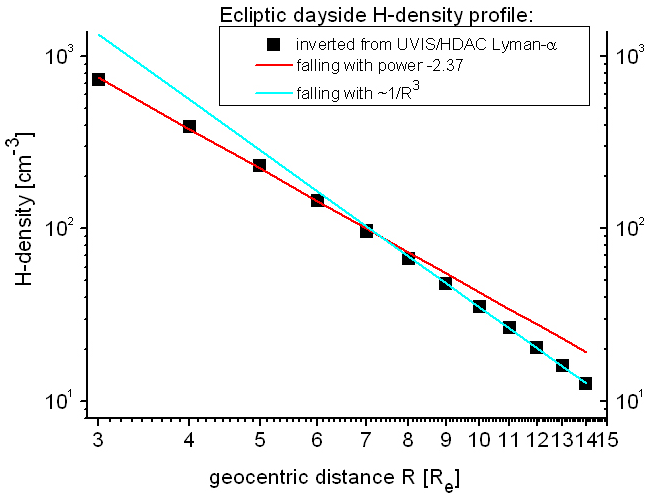
Figure 4(Black squares): radial symmetric H-density profile (Eq. 7) fitted from UVIS/HDAC observations; (red line): power-law fit of the H-density profile in the lower radial range 3–7 RE; (cyan line): power-law fit of the H-density profile in the upper radial range 9–15 RE. The deviation in the red and the cyan lines from the black squares indicates that the H-density profiles fall faster at larger distances > 8 RE than at lower distances < 8 RE.
Obvious in Fig. 4 is a change in the radial dependency of the profile in the radial region above 8 RE. At distances lower than 8 RE, the H-density profile seems to fall off with distance with a power law, i.e., ≈ r−2.37 (red line in Fig. 4). It was fitted in the distance range 3–7 RE:
where the geocentric distance r is in RE. The black and red lines are in very good agreement at 3–7 RE. Above > 8 RE the situation has changed, and the H density falls off with a rate ≈ r−3, which is indicated by the very good agreement between the cyan and the black squares there. The fit of the H-density profile between 9–15 RE delivers a r−3 fall:
From theory, an enhanced loss of neutral H atoms near the magnetopause and outside the magnetosphere can be expected due to sharply increased interactions with solar wind ions in this region that produce soft X-ray photons and ENA observations. The faster decrease with r−3 in the H-density profile above 8 RE might indicate the higher ionization of cold exospheric neutrals near the magnetopause (located at 9–11 RE in the vicinity of the subsolar point) and beyond.
From the fitted H-density profile of Eq. (7), the exospheric H density at 10 RE was found to be 35 cm−3 at the ecliptic dayside. From known variations of the neutral exosphere due to geomagnetic storms up to 20 % (Zoennchen et al., 2017) and with the summarized error from other contributions (i.e. from background, solar Lyman-α flux, and so on), there is an expected total error in the H density of about 25 %. Nevertheless, from several facts we assume that the found value of 35 cm−3 at 10 RE is more likely to be a lower limit. First, between 3–10 RE the neutral exospheric response to geomagnetic storms is so-far known as an increase and not as a decrease of neutral density (Bailey and Gruntman, 2013; Zoennchen et al., 2017; Cucho-Padin and Waldrop, 2019). Second, there are indications that an increasing solar activity also corresponds to an increase of neutral density in this radial range, either weak (Fuselier et al., 2020) or somewhat stronger (Zoennchen et al., 2015). The H-density model from TWINS used here is based on observations in 2008 and 2010 near solar minimum during quiet days without storms. Therefore, it likely represents an exosphere with neutral densities close to their lowest values.
Ecliptic dayside Lyman-α observations of the terrestrial H exosphere between 3–15 RE by UVIS/HDAC aboard CASSINI were compared to calculated Lyman-α brightnesses using two different H-density models: first, the H-density model based on TWINS Lyman-α observations from 2008 and 2010 and second the model introduced by Chamberlain (1963). The calculations considered the HDAC Lyman-α observations, CASSINI's trajectory, and the HDAC LOS published by Werner et al. (2004).
As first result, it was found that the radial dependence of the HDAC observations and the calculated profile from the TWINS model are very similar in the radial range 3–8 RE. The model shows significant deviations from the observed profile in this lower range.
To be able to convert the HDAC observations from counts per second into physical units [R], the averaged conversion factor fc=3.285 counts s−1 R−1 was derived in the radial range 3.0–5.5 RE (overlapping region) from the ratio between the HDAC observations and the calculated Lyman-α brightnesses from the TWINS model. Dayside LOSs with impact distances in the overlapping region are available from both instruments – HDAC and TWINS LAD. Additionally a second independent way was used to quantify the conversion factor fc=3.215 counts s−1 R−1 by calculating the ratio between the estimated background value given by Werner et al. (2004) and the corresponding value taken from the SOHO/SWAN map. Both values found for fc are very close together.
With usage of fc=3.285, the HDAC observations are inverted into a radial symmetric H-density profile of the ecliptic dayside between 3–15 RE. The derived density profile determined a H-density value of 35 cm−3 at 10 RE in the vicinity of the subsolar point. The error is expected with 25 %. Nevertheless, from different mentioned reasons, it is more likely that this value is closer to the lower limit.
Also found was a faster decrease in the H density for distances above 8 RE (r−3) compared to the lower region of 3–7 RE (r−2.37). This is consistent with an enhanced depletion of neutral H in the far-upsun direction beyond 8 RE reported by Carruthers et al. (1976) based on Lyman-α images from the Moon by Apollo 16 and also with observations of Mariner 5 (Wallace et al., 1970).
The faster H-density decrease above 8 RE in the upsun direction as quantified in this study may indicate an enhanced ionization rate near the magnetopause and beyond, due to sharply increased interactions there of neutral H atoms with solar wind ions.
The regions near the subsolar point (close to the magnetopause) and the connected magnetosheath are identified as sources of observable, strong, enhanced ENA production (see Fuselier et al., 2010, 2020) and of soft X-ray radiation (see Connor and Carter, 2019).
The ENAs are produced by charge exchange between energized solar wind H+ ions and cold geocoronal neutral H. The result is a slow H+ ion (bound to the terrestrial magnetic field) and a fast, neutral H atom (ENA), which mainly escapes from this region into space.
The soft X-ray radiation is (also) produced by charge exchange – between highly charged solar wind oxygen ions (O7+ or O8+) and geocoronal neutral H, which donates an electron to the ions (referred to as solar wind charge exchange, SWCX).
Inside the magnetopause there is a protection against the solar wind ions due to the terrestrial magnetic field. This situation changes from the magnetopause towards the connected magnetosheaths. There, the named ENA and soft X-ray production sharply increases, since the solar wind ions can penetrate this regions.
In both processes cold, neutral H atoms are lost by conversion into ions. This might be a possible reason for a faster decrease in the neutral geocoronal H density in the named regions of ENA or soft X-ray production.
The underlying software code is not publicly accessible. It is embedded in a much larger program for the reduction and analysis of Lyman-α raw data from TWINS and other spacecraft. The packages as well as their functions and subroutines are from libraries that are partly commercial or have separate copyright notes from their creators. For the future, our plan is to replace all usage of external code with our own code; however, until this is done, the software can not be made publicly accessible.
The following datasets were used in this paper:
-
interplanetary SOHO Lyman-α background map provided by LATMOS-IPSL, Université de Versailles Saint-Quentin-en-Yvelines, CNRS, France (http://swan.projet.latmos.ipsl.fr/images/, LATMOS, 2022);
-
total solar Lyman-α flux provided by LASP (Laboratory For Atmospheric And Space Physics), University of Colorado Boulder (https://lasp.colorado.edu/lisird/data/composite_lyman_alpha/, LISIRD, 2022);
-
dst-index provided by World Data Center for Geomagnetism, Kyoto, Japan (https://wdc.kugi.kyoto-u.ac.jp/dstdir/, World Data Center for Geomagnetism, Kyoto, 2022);
-
solar F10.7 cm radio flux provided by CLS, France (https://spaceweather.cls.fr/services/radioflux/, CLS, 2022).
No other datasets are used in the paper. The UVIS/HDAC data were analyzed by Werner et al. (2004); we did not access these data and used only a numerical approximation (see Eq. 1) of the Lyman-α profile presented in Fig. 2 of Werner et al. (2004). Furthermore, no TWINS data were analyzed here; we only used the model coefficients of the TWINS H-density model published in Zoennchen et al. (2015) and the local Lyman-α illumination map (Fig. 2) for the calculations.
JHZ conceived the initial idea, carried out the calculations, and wrote the initial draft of the paper. HKC contributed important ideas, wrote Sect. 1 of the paper, and was involved in drafting the paper and revising it critically for important aspects. JJ was involved in revising numerical approximations and critically coordinated transformations. UN and HJF approved the final version of the paper to be published.
The contact author has declared that neither they nor their co-authors have any competing interests.
Publisher's note: Copernicus Publications remains neutral with regard to jurisdictional claims in published maps and institutional affiliations.
The authors gratefully thank the TWINS team (Dave McComas) for making this work possible. Jochen Zoennchen gratefully acknowledges the funding by the Deutsche Forschungsgemeinschaft (DFG, German Research Foundation) 469043535. Hyunju K. Connor gratefully acknowledges support from the NSF grants AGS-1928883 and OIA-1920965 and the NASA grants 80NSSC18K1042, 80NSSC18K1043, 80NSSC19K0844, 80NSSC20K1670, and 80MSFC20C0019. We acknowledge the support from the International Space Science Institute on the ISSI team 492, titled “The Earth's Exosphere and its Response to Space Weather”. Additionally, we thank the topical editor and the referees for the discussions and the extensive help with improving the paper.
This research has been supported by the Deutsche Forschungsgemeinschaft (grant no. 469043535), the National Science Foundation (grant nos. AGS-1928883 and OIA-1920965), the National Aeronautics and Space Administration (grant nos. 80NSSC18K1042, 80NSSC18K1043, 80NSSC19K0844, 80NSSC20K1670, and 80MSFC20C0019).
This open-access publication was funded
by the University of Bonn.
This paper was edited by Petr Pisoft and reviewed by Joseph D. Perez and one anonymous referee.
Bailey, J. and Gruntman, M.: Experimental study of exospheric hydrogen atom distributions by Lyman-α detectors on the TWINSmission, J. Geophys. Res., 116, A09302, https://doi.org/10.1029/2011JA016531, 2011.
Bailey, J. and Gruntman, M.: Observations of exosphere variations during geomagnetic storms, Geophys. Res. Lett., 40, 1907–1911, https://doi.org/10.1002/grl.50443, 2013.
Baliukin, I., Bertaux, J.-L., Quemerais, E., Izmodenov, V., and Schmidt, W.: SWAN/SOHO Lyman-α mapping: The hydrogen geocorona extends well beyond the Moon, J. Geophys. Res.-Space, 124, 861–885, https://doi.org/10.1029/2018JA026136, 2019.
Beth, A., Garnier, P., Toublanc, D., Dandouras, I., and Mazelle, C.: Theory for planetary exospheres: II. Radiation pressure effect on exospheric density profiles, Icarus, 266, 423–432, https://doi.org/10.1016/j.icarus.2015.08.023, 2016.
Bishop, J.: Geocoronal structure: The effect of solar radiation pressure and plasmasphere interaction, J. Geophys. Res., 90, 5235–5245, 1985.
Branduardi-Raymont, G., Wang, C., Escoubet, C. P., Adamovic, M., Agnolon, D., Berthomier, M., Carter, J. A., Chen, W., Colangeli, L., Collier, M., Connor, H. K., Dai, L., Dimmock, A., Djazovski, O., Donovan, E., Eastwood, J. P., Enno, G., Giannini, F., Huang, L., Kataria, D., Kuntz, K., Laakso, H., Li, J., Li, L., Lui, T., Loicq, J., Masson, A., Manuel, J., Parmar, A., Piekutowski, T., Read, A. M., Samsonov, A., Sembay, S., Raab, W., Ruciman, C., Shi, J. K., Sibeck, D. G., Spanswick, E. L., Sun, T., Symonds, K., Tong, J., Walsh, B., Wei, F., Zhao, D., Zheng, J., Zhu, X., and Zhu, Z.: SMILE Definition study report (red book), ESA/SCI(2018)1, https://sci.esa.int/web/smile/-/61194-smile-definition-study-report-red-book (last access: 1 November 2021), 2018.
Carruthers, G. R., Page, T., and Meier, R. R.: Apollo 16 Lyman alpha imagery of the hydrogen geocorona, J. Geophys. Res., 81, 1664–1672 https://doi.org/10.1029/JA081i010p01664, 1976.
Chamberlain, J. W.: Planetary coronae and atmospheric evaporation, Planet Space Sci., 11, 901–960, 1963.
CLS: Solar radio flux for orbit determination: nowcast and forecast, Collecte Localisation Satellites [data set], https://spaceweather.cls.fr/services/radioflux/, last access: 10 April 2022.
Connor, H. K. and Carter, J. A.: Exospheric neutral hydrogen density at the 10 Re subsolar point deduced from XMM-Newton X-ray observations, J. Geophys. Res.-Space, 124, 1612–1624, https://doi.org/10.1029/2018JA026187, 2019.
Connor, H. K., Sibeck, D. G., Collier, M. R., Baliukin, I. I., Branduardi-Raymont, G., Brandt, P. C., Buzulukova, N. Y., Collado-Vega, Y. M., Escoubet, C. P., Fok, M.-C., Hsieh, S.-Y., Jung, J., Kameda, S., Kuntz, K. D., Porter, F. S., Sembay, S., Sun, T., Walsh, B. M., and Zoennchen, J. H.: Soft X-ray and ENA imaging of the Earth's dayside magnetosphere, J. Geophys. Res.-Space, 126, e2020JA028816, https://doi.org/10.1029/2020JA028816, 2021.
Cucho-Padin, G. and Waldrop, L.: Time-dependent Response of the Terrestrial Exosphere to a Geomagnetic Storm, Geophys. Res. Lett., 46, 11661–11670, https://doi.org/10.1029/2019GL084327, 2019.
Domingo, V., Fleck, B., and Poland, A. I.: SOHO: The solar and heliospheric observatory, Space Sci. Rev., 72, 81–84, https://doi.org/10.1007/BF00768758, 1995.
Emerich, C., Lemaire, P., Vial, J.-C., Curdt, W., Schühle, U., and Wilhelm, K.: A new relation between the central spectral solar HI Lyman-α irradiance and the line irradiance measured by SUMER/SOHO during the cycle 23, Icarus, 178, 429–433, https://doi.org/10.1016/j.icarus.2005.05.002, 2005.
Fahr, H. J., Nass, U., Dutta-Roy, R., and Zoennchen, J. H.: Neutralized solar wind ahead of the Earth's magnetopause as contribution to non-thermal exospheric hydrogen, Ann. Geophys., 36, 445–457, https://doi.org/10.5194/angeo-36-445-2018, 2018.
Fuselier, S. A., Funsten, H. O., Heirtzler, D., Janzen, P., Kucharek, H., McComas, D. J., Möbius, E., Moore, T. E., Petrinec, S. M., Reisenfeld, D. B., Schwadron, N. A., Trattner, K. J., and Wurz, P.: Energetic neutral atoms from the Earth's sub-solar magnetopause, Geophys. Res. Lett., 37, L13101, https://doi.org/10.1029/2010GL044140, 2010.
Fuselier, S. A., Dayeh, M. A., Galli, A., Funsten, H. O., Schwadron, N. A., Petrinec, S. M., Trattner, K. J., McComas, D. J., Burch, J. L., Toledo-Redondo, S., Szalay, J. R., and Strangeway, R. J.: Neutral atom imaging of the solar wind-magnetosphere-exosphere interaction near the subsolar magnetopause, Geophys. Res. Lett., 47, e2020GL089362, https://doi.org/10.1029/2020GL089362, 2020.
Goldstein, J. and McComas, D. J.: The big picture: Imaging of the global geospace environment by the TWINS mission, Rev. Geophys., 56, 251–277, https://doi.org/10.1002/2017RG000583, 2018.
Hodges Jr., R. R.: Monte Carlo simulation of the terrestrial hydrogen exosphere, J. Geophys. Res., 99, 23229–23247, 1994.
Jansen, F., Lumb, D., Altieri, B., Clavel, J., Ehle, M., Erd, C., Gabriel, C., Guainazzi, M., Gondoin, P., Much, R., Munoz, R., Santos, M., Schartel, N., Texier, D., and Vacanti, G.: XMM-Newton observatory: I. The spacecraft and operations, Astron. Astrophys., 365, L1–L6, https://doi.org/10.1051/0004-6361:20000036, 2001.
Kusnierkiewicz, D. Y.: A description of the TIMED spacecraft, American Institute of Physics (AIP) Conference Proceedings, 387, Part One, 115–121, https://doi.org/10.1063/1.51934, 1997.
LATMOS: Summary Images, LATMOS-IPSL [data set], http://swan.projet.latmos.ipsl.fr/images/, last access: 10 April 2022.
LISIRD: Composite Solar Lyman-alpha, Time Series, LASP Interactive Solar Irradiance Datacenter [data set], https://lasp.colorado.edu/lisird/data/composite_lyman_alpha/, last access: 10 April 2022.
McComas, D. J., Allegrini, F., Bochsler, P., Bzowski, M., Christian, E. R., Crew, G. B., DeMajistre, R., Fahr, H., Fichtner, H., Frisch, P. C., Funsten, H. O., Fuselier, S. A., Gloeckler, G., Gruntman, M., Heerikhuisen, J., Izmodenov, V., Janzen, P., Knappenberger, P., Krimigis, S., Kucharek, H., Lee, M., Livadiotis, G., Livi, S., MacDowall, R. J., Mitchell, D., Möbius, E., Moore, T., Pogorelov, N. V., Reisenfeld, D., Roelof, E., Saul, L., Schwadron, N. A., Valek, P. W., Vanderspek, R., Wurz, P., and Zank, G. P.: Global observations of the interstellar interaction from the Interstellar Boundary Explorer (IBEX), Science, 326, 959–962, https://doi.org/10.1126/science.1180906, 2009.
Qin, J. and Waldrop, L.: Non-thermal hydrogen atoms in the terrestrial upper thermosphere, Nat. Commun., 7, 13655, https://doi.org/10.1038/ncomms13655, 2016.
Qin, J., Waldrop, L., and Makela, J. J.: Redistribution of H atoms in the upper atmosphere during geomagnetic storms, J. Geophys. Res.-Space, 122, 10686–10693, https://doi.org/10.1002/2017JA024489, 2017.
Rairden, R. L., Frank, L. A., and Craven, J. D.: Geocoronal imaging with Dynamics Explorer, J. Geophys. Res., 91, 13613–13630, https://doi.org/10.1029/JA091iA12p13613, 1986.
Sibeck, D. G., Allen, R., Aryan, H., Bodewits, D., Brandt, P., Branduardi-Raymont, G., Brown, G., Carter, J. A., Collado-Vega, Y. M., Collier, M. R., Connor, H. K., Cravens, T. E., Ezoe, Y., Fok, M.-C., Galeazzi, M., Gutynska, O., Holmström, M., Hsieh, S.-Y., Ishikawa, K., Koutroumpa, D., Kuntz, K. D., Leutenegger, M., Miyoshi, Y., Porter, F. S., Purucker, M. E., Read, A. M., Raeder, J., Robertson, I. P., Samsonov, A. A., Sembay, S., Snowden, S. L., Thomas, N. E., von Steiger, R., Walsh, B. M., and Wing, S.: Imaging plasma density structures in the soft X-rays generated by solar wind charge exchange with neutrals, Space Sci. Rev., 214, 79, https://doi.org/10.1007/s11214-018-0504-7, 2018.
Waldrop, L. and Paxton, L. J.: Lyman-α airglow emission: Implications for atomic hydrogen geocorona variability with solar cycle, J. Geophys. Res.-Space, 118, 5874–5890, https://doi.org/10.1002/jgra.50496, 2013.
Wallace, L., Barth, C. A., Pearce, J. B., Kelly, K. K., Anderson, D. E., and Fastie, W. G.: Mariner 5 measurement of the Earth's Lyman alpha emission, J. Geophys. Res., 75, 3769–3777, https://doi.org/10.1029/JA075i019p03769, 1970.
Werner, S., Keller, H. U., Korth, A., and Lauche, H.: UVIS/HDAC Lyman-α observations of the geocorona during Cassini's Earth swingby compared to model predictions, Adv. Space Res., 34, 1647–1649, https://doi.org/10.1016/j.asr.2003.03.074, 2004.
Woods, T. N., Tobiska, W. K., Rottman, G. J., and Worden, J. R.: Improved solar Lyman alpha irradiance modeling from 1947 through 1999 based on UARS observations, J. Geophys. Res., 105, 27195–27215, https://doi.org/10.1029/2000JA000051, 2000.
World Data Center for Geomagnetism, Kyoto: Geomagnetic Equatorial Dst index Home Page, World Data Center for Geomagnetism, Kyoto [data set], https://wdc.kugi.kyoto-u.ac.jp/dstdir/, last access: 10 April 2022.
Zoennchen, J. H., Bailey, J. J., Nass, U., Gruntman, M., Fahr, H. J., and Goldstein, J.: The TWINS exospheric neutral H-density distribution under solar minimum conditions, Ann. Geophys., 29, 2211–2217, https://doi.org/10.5194/angeo-29-2211-2011, 2011.
Zoennchen, J. H., Nass, U., and Fahr, H. J.: Exospheric hydrogen density distributions for equinox and summer solstice observed with TWINS1/2 during solar minimum, Ann. Geophys., 31, 513–527, https://doi.org/10.5194/angeo-31-513-2013, 2013.
Zoennchen, J. H., Nass, U., and Fahr, H. J.: Terrestrial exospheric hydrogen density distributions under solar minimum and solar maximum conditions observed by the TWINS stereo mission, Ann. Geophys., 33, 413–426, https://doi.org/10.5194/angeo-33-413-2015, 2015.
Zoennchen, J. H., Nass, U., Fahr, H. J., and Goldstein, J.: The response of the H geocorona between 3 and 8 Re to geomagnetic disturbances studied using TWINS stereo Lyman-α data, Ann. Geophys., 35, 171–179, https://doi.org/10.5194/angeo-35-171-2017, 2017.
- Abstract
- Introduction
- The UVIS/HDAC Lyman-α observations during CASSINI's swing-by maneuver at the Earth
- Solar conditions and the interplanetary Lyman-α background
- Approach
- Comparison of the observed UVIS/HDAC profile with calculated profiles
- H-density profile derived from the UVIS/HDAC observations
- Discussion
- Code availability
- Data availability
- Author contributions
- Competing interests
- Disclaimer
- Acknowledgements
- Financial support
- Review statement
- References