the Creative Commons Attribution 4.0 License.
the Creative Commons Attribution 4.0 License.
 | 22 Apr 2022
High bandwidth measurements of auroral Langmuir waves with multiple antennas
Chrystal Moser
James LaBelle
Iver H. Cairns
The High-Bandwidth Auroral Rocket (HIBAR) was launched from Poker Flat, Alaska, on 28 January 2003 at 07:50 UT towards an apogee of 382 km in the nightside aurora. The flight was unique in having three high-frequency (HF) receivers using multiple antennas parallel and perpendicular to the ambient magnetic field, as well as very low-frequency (VLF) receivers using antennas perpendicular to the magnetic field. These receivers observed five short-lived Langmuir wave bursts lasting from 0.1–0.2 s, consisting of a thin plasma line with frequencies in the range of 2470–2610 kHz that had an associated diffuse feature occurring 5–10 kHz above the plasma line. Both of these waves occurred slightly above the local plasma frequency with amplitudes between 1–100 µV m−1. The ratio of the parallel to perpendicular components of the plasma line and diffuse feature were used to determine the angle of propagation of these waves with respect to the background magnetic field. These angles were found to be comparable to the theoretical Z-infinity angle that these waves would resonate at. The VLF receiver detected auroral hiss throughout the flight at 5–10 kHz, a frequency matching the difference between the plasma line and the diffuse feature. A dispersion solver, partially informed with measured electron distributions, and associated frequency- and wavevector-matching conditions were employed to determine if the diffuse features could be generated by a nonlinear wave–wave interaction of the plasma line with the lower-frequency auroral hiss waves/lower-hybrid waves. The results show that this interpretation is plausible.
- Article
(9863 KB) - Full-text XML
- BibTeX
- EndNote


Plasma waves generated at or near the local plasma frequency have been observed in the auroral ionosphere by satellites and rockets ever since there have been instruments capable of measuring them (review by Akbari et al., 2021). These wave amplitudes can range from a few millivolts per meter (mV m−1) (McFadden et al., 1986) to greater than 1 V m−1 (Kintner et al., 1995) and have been observed in both under- (fpe<fce) and over-dense (fpe>fce) plasmas, where fpe is the electron plasma frequency and fce is the electron cyclotron frequency (Beghin et al., 1989; McAdams et al., 1999). Simultaneous observations of electron distribution functions and plasma waves have been reported by McFadden et al. (1986), Ergun et al. (1991), and Beghin et al. (1989). Langmuir waves can be generated by both electrons accelerated by parallel electric fields in the auroral acceleration region and scattered into a broad downgoing beam or by concentrated parallel electron beams caused by Alfvénic acceleration. Beghin et al. (1989) also showed that frequency structures within the waves occur often in the auroral ionosphere, with an 80 % occurrence rate on the dayside and 60 % on the nightside. More recent observations of Langmuir waves by the TRICE-1 (Twin Rockets to Investigate Cusp Electrodynamics) sounding rocket were reported by LaBelle et al. (2010), with modulations as low as 1 kHz and up to tens of kilohertz (kHz) in an under-dense plasma.
McAdams and LaBelle (1999) and Samara and LaBelle (2006) observed structured spectral peaks above the plasma frequency in high-frequency (HF) spectrograms. The former dubbed these bursts “chirps”, with amplitudes up to 1 mV m−1 relatively close to fpe, and with similar amplitude diffuse waves occurring above the chirp signal. The latter reported several similar observations made by the SIERRA (Sounding of the Ion Energization Region: Resolving Ambiguities), PHAZE II (Physics of Auroral Zone Electrons), and RACE (Rocket Auroral Correlator Experiment) sounding rockets, all of which were in an over-dense plasma. These were investigated theoretically by McAdams et al. (2000), who interpreted them as linear eigenmodes in preexisting density structures. Similar Langmuir eigenmodes have subsequently been observed in the solar wind (Malaspina et al., 2008; Ergun et al., 2008).
Evidence for nonlinear processes has been reported, as recently reviewed by Akbari et al. (2021). In addition to these various weak turbulence phenomena discussed above, there is evidence for strong turbulence phenomena in aurora, such as Langmuir cavitons (Akbari et al., 2013), as well as for electron and ion phase space holes (Ergun et al., 1998; Schamel et al., 2020; review by Akbari et al., 2021). Stasiewicz et al. (1996), using Freja satellite data, observed evidence of both parametric decay of a Langmuir wave into a lower- hybrid (LH) wave and an oblique wave (L′), via the process , and scattering off an existing LH wave (e.g., ), confirmed by Lizunov et al. (2001) and Khotyaintsev et al. (2001). A model based on scattering of the plasma wave with an electrostatic whistler/lower-hybrid wave is put forth as a plausible explanation for the modulations observed by Freja and SCIFER (Sounding of the Cusp Ion Fountain Energization Region) (Bonnell et al., 1997). Cairns and Layden (2018) reviewed the decay process of generalized Langmuir waves into backscattered Langmuir waves and either ion acoustic waves or ion cyclotron waves and showed, in a strongly magnetized plasma (fpe<fce), the backscattered Langmuir wavenumber is greater than the initial Langmuir wavenumber, . Other nonlinear processes have been observed and studied in the auroral ionosphere involving Langmuir waves and whistler-mode waves. Böhm et al. (1990) presented observation from two sounding rockets of intense Langmuir and whistler waves and showed they were associated with Alfvén waves. This process was shown to be theoretically feasible through the parametric decay of Langmuir waves into whistler (W) and Alfvén electromagnetic ion-cyclotron (EMIC) waves (A), () (Chian et al., 1994; Lopes and Chian, 1996). This theory could also be relevant to the observations of EMIC waves by the Auroral Turbulence sounding rocket reported by Lund and LaBelle (1997), who reviewed Langmuir turbulence in the auroral ionosphere induced by electron beams instabilities and ion density irregularities that result in the parametric decay of Langmuir waves into secondary Langmuir waves and ion acoustic waves, .
McFadden et al. (1986) measured both parallel and perpendicular components of the electric field, observing Langmuir waves with larger parallel components such that , that were coincident with unstable parallel electron distributions. Colpitts and LaBelle (2008) performed a Monte Carlo simulation of the Langmuir and Z-mode waves and showed their electric fields are preferentially parallel, becoming more perpendicular as the frequencies increased towards the upper-hybrid (UH) frequency as expected. Dombrowski et al. (2012) used the unique 3-D data set from TRICE-1 to determine the intensity of the electric field for Langmuir waves and showed their parallel components are more than 2 times larger than their perpendicular components.
The High-Bandwidth Auroral Rocket (HIBAR) was one in a series of sounding rockets equipped with the telemetry capable of measuring high-frequency waves in detail. Uniquely, it achieved these measurements in both the parallel and perpendicular direction with respect to the background magnetic field, which allows for the identity of the wave mode (e.g., parallel propagating Langmuir wave or perpendicularly propagating upper-hybrid mode) and the direction of propagation of the different waves to be determined and compared with theory. Its goal was to measure waves generated by intense beams of electron precipitating down the magnetic field at high latitudes in the F region of the ionosphere, where fpe<fce. Previously, Samara et al. (2004) analyzed UH waves from HIBAR at the condition fUH=2fce, where fUH is the upper-hybrid (UH) frequency, the source of auroral roar emissions seen at ground level (review by LaBelle and Treumann, 2002). This report presents observations by the HIBAR mission of Langmuir wave bursts near fpe, with a region of diffuse waves occurring at a frequencies 5–15 kHz above the plasma bursts, as well as low-frequency whistler-mode hiss occurring between 5–15 kHz. The wave events are observed in the over-dense regime. Using a wave dispersion solver to determine the normal modes of the waves and the growth rates for the normal modes, we will show these waves could plausibly be generated by a wave–wave interaction of the Langmuir wave with low-frequency waves in the lower-hybrid mode.
HIBAR was launched from Poker Flat, Alaska, on 28 January 2003, at 07:50 UT into active pre-midnight aurora, reaching an apogee of 382 km. The geomagnetic field was strongly perturbed, exhibiting a sequence of 50–100 nT magnetic bays in the north–south component, the first of which coincided with the rocket launch, indicating that an expansion phase or pseudo breakup was in progress. Its payload included a Langmuir probe, particle detectors, and DC (direct current), very low-frequency (VLF), and HF electric field receivers. HIBAR was one in a series of rockets with a high telemetry rate to measure waves with frequencies up to 5 MHz, allowing for observations of detailed structure of high-frequency waves in the lower ionosphere, such as Langmuir and upper-hybrid (UH) waves. The rocket's spin axis was aligned to within 5∘ of the background magnetic field, with a spin rate of 0.95 Hz. For wave measurements, the rocket included two radial booms oriented perpendicular to one another and three axial booms, one along the axis of the rocket protruding from the front deck and two mounted on the ends of the radial booms (see Fig. 1).
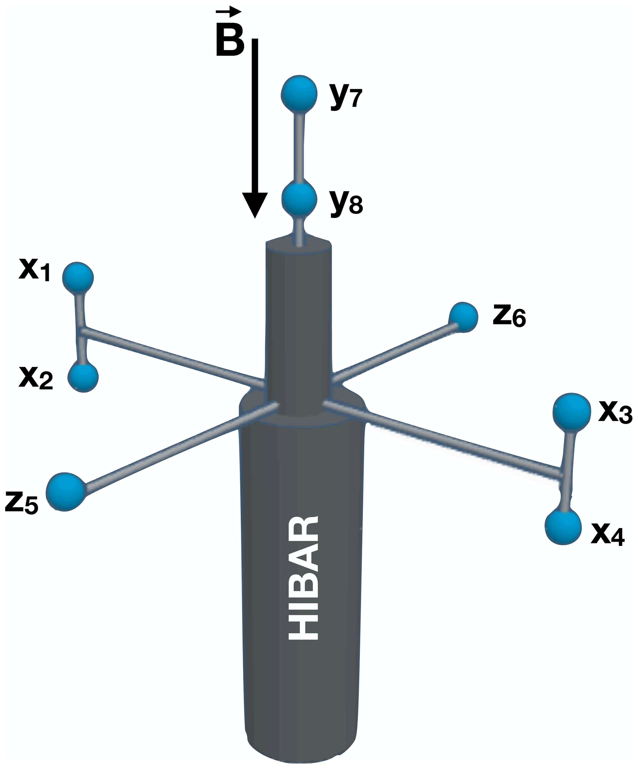
Figure 1Diagram of the HIBAR rocket showing approximate antenna orientations with respect to the background magnetic field (note that the labeling of the probes has no connection to Cartesian coordinates).
The unique feature of HIBAR was the large number of HF telemetry links. Among these, two were dedicated to measurements of components of HF wave electric fields up to 5 MHz: the perpendicular electric field used probes x1 and x3, located 2.5 m apart oriented perpendicular to the rocket axis, and the parallel electric field used probes x1 and x2, located 0.28 m apart and oriented along the rocket axis. Voltage differences between these probe pairs, amplified and filtered, modulated dedicated transmissions from rocket to ground station. An automatic gain control (AGC) was used to optimize dynamic range. The AGC level was transmitted as a separate pulse code modulation (PCM) link and combined with the HF signal post analysis. Four electrostatic analyzers (ESAs) measured ion and electron energies from 70 eV to 19 keV at eight pitch angles from 0–180∘, sweeping through the energy steps every 45 ms.
Figure 2a and b show HF spectrograms from both perpendicular and parallel antennas covering 07:54:13–07:54:33 UT (253–273 s) flight time and the altitude range to ∼364–374 km, one of the intervals when Langmuir waves were observed. Figure 2c and d show data for a slightly later interval, 07:55:49–07:56:09 UT (349–369 s), corresponding to 377–370 km altitude, which also contains Langmuir waves. As usual, plasma noise is enhanced in the band between fpe and fUH, so that the local plasma frequency can be seen as lower cutoffs in both the spectrograms between 2400 and 2700 kHz and the upper-hybrid frequency can be seen as an upper cutoff in the perpendicular spectrograms between 2800 and 3000 kHz. During these two time intervals, HIBAR encountered seven short-lived wave bursts near fpe that last from ∼0.1–0.2 s, five of which had a diffuse band occurring 5–10 kHz above a narrow plasma wave line (see Fig. 4) and well below the upper-hybrid band above 2800 kHz. These five events are labeled in Fig. 2 by their respective times (in seconds after launch), occurring at 07:54:20, 07:54:22, and 07:54:32 in Fig. 2a and b and 07:55:51 and 07:55:59 UT in Fig. 2c and d. For the entirety of both intervals in Fig. 2, HIBAR is in over-dense plasma (fpe>fce).
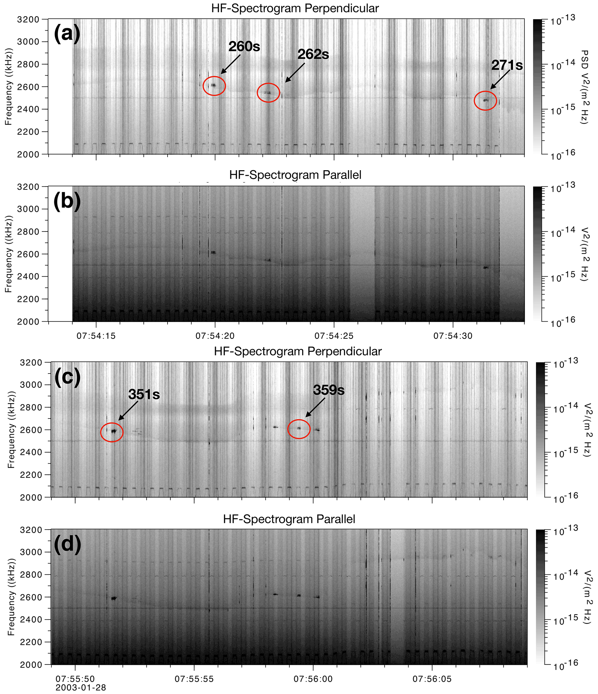
Figure 2The 2000–3200 kHz spectrograms of perpendicular (upper panels a and c) and parallel (lower panels b and d) HF electric fields for two time intervals during the HIBAR rocket flight, 07:54:18–07:54:33 UT and 07:55:49–07:36:04 UT, showing the plasma frequency cutoff as a lower bound in the perpendicular and parallel spectrograms and the upper-hybrid frequency cutoff as an upper bound in the perpendicular spectrograms. Red circles indicate five Langmuir wave bursts used for detailed study.
Figure 3 shows the very low-frequency (VLF) data in a frequency-time spectrogram for the interval when the Langmuir wave bursts are seen, between 07:54:10–07:56:10 UT (250–370 s) and ∼360–380 km. There is a broadband enhancement of the whistler-mode waves between 4–15 kHz, with a small band of slightly more enhanced waves at approximately 5 kHz, believed to be near the LH frequency because it acts as a cutoff to the whistler mode. These waves were measured with a separate perpendicular antenna, oriented 90∘ to the antennas used to measured the HF waves, using probes z5 and z6 in Fig. 1.
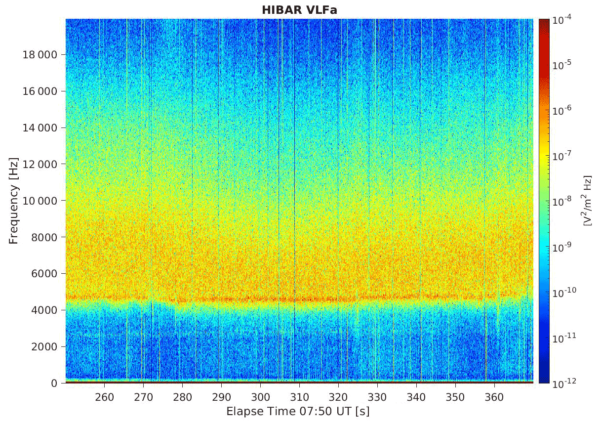
Figure 3Frequency–power spectrogram of the HIBAR VLF wave data from 0–20 kHz and 07:54:10–07:56:10 UT (250–370 s), showing the broadband diffuse whistler-mode waves and a slightly enhanced power band at ∼5 kHz corresponding to probable LH waves.

Figure 4Enhanced plots of the five Langmuir bursts indicated in Fig. 2, presented in time order, each comprised of a narrow band plasma line and a broadband diffuse feature with ∼5–15 kHz higher frequency. The top panels in each plot are from the perpendicular antenna, the middle panels are from the parallel antenna, and the bottom panels are the parallel to perpendicular ratios of the amplitudes of the plasma peaks (red) and the diffuse feature (blue).
Figure 4 shows enhanced spectrograms of five selected Langmuir wave events observed by both the parallel and perpendicular HF antenna, labeled 260s, 262s, 271s, 351s, and 359s in Fig. 2. These events include a thin, intense plasma line just above the plasma frequency cutoff and a less intense band of waves above the plasma line, referred to as the diffuse feature. Other plasma line events occurred during HIBAR; however, these did not include the diffuse waves and therefore were not considered in this study. Obtaining absolute units for the electric fields of these features requires the AGC voltage data to be combined with the raw HF waveform data. These values were then divided by the length of the respective booms to obtain electric fields in volts per meter (V m−1), under the assumption, discussed below, that the wavelength is longer than the probe separation.
Black boxes in each spectrogram in Fig. 4 outline time and frequency intervals used to calculated average intensities of the plasma line and diffuse features of each event. Figure 5 shows details of this calculation for a selected event, shown in Fig. 4a as occurring at 259.9–260.0 s. Separately for both the parallel and perpendicular spectra, the background power spectral density level was determined for each event by computing the average spectral density over a slightly higher-frequency range, as indicated by the upper black box spanning 2640–2660 kHz in Fig. 5a and b. The background interval was selected separately and was slightly different for each of the other four events shown in Fig. 4. For each event, a spectrum was produced by subtracting this average background power spectral density from each spectrum. Figure 5c shows example spectra after this subtraction, for both perpendicular (blue trace) and parallel (red trace) waves for the time indicated by a vertical red line in Fig. 5a and b. This was done because the background noise, either from the instrument or from the environment, was significantly different between the two antennas and would have affected the ratio of the electric fields. It was removed for a more accurate estimate of the ratio of the parallel to perpendicular electric fields.
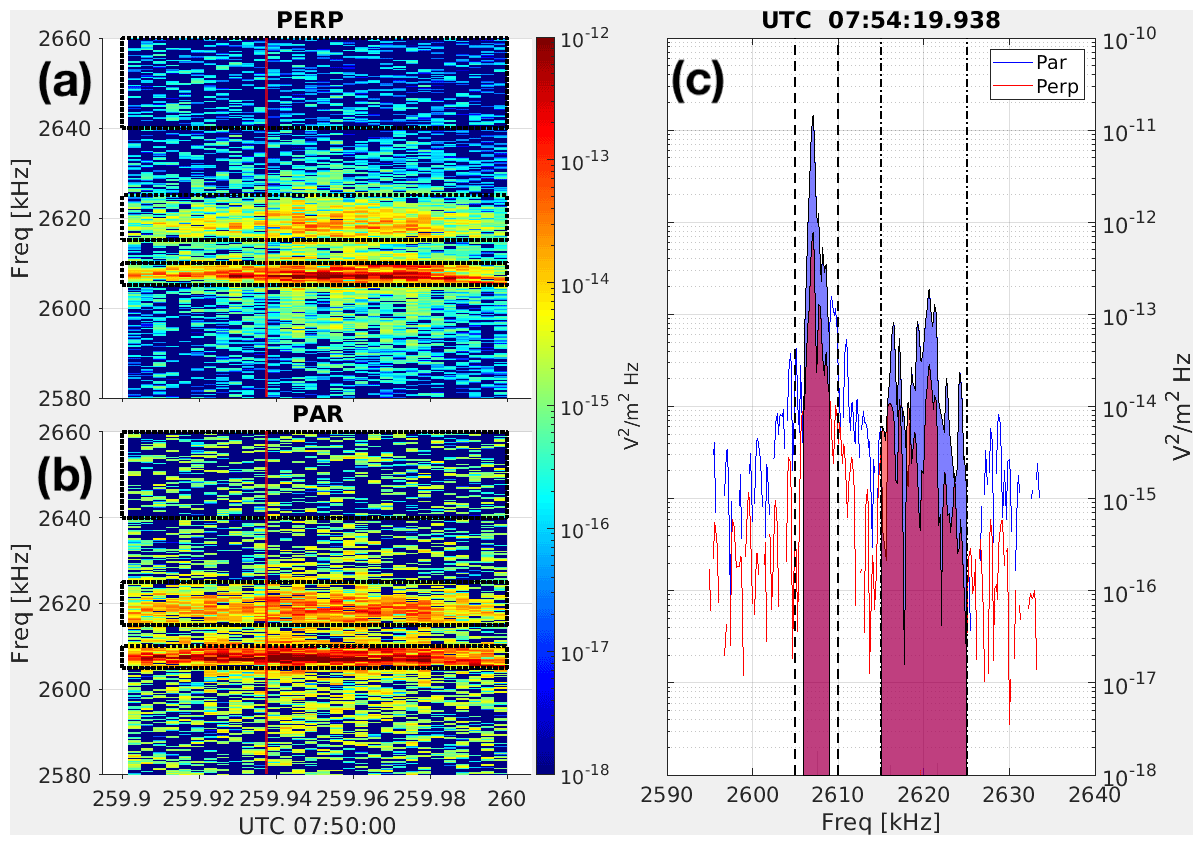
Figure 5(a) Perpendicular and (b) parallel spectrograms for the Langmuir bursts labeled 260s in Fig. 2 and shown in Fig. 4a. Black boxes indicate the frequency–time ranges used to define the plasma line, diffuse feature, and background level. (c) Selected spectrum with background noise subtracted, occurring at the time highlighted as a red vertical line in panels (a) and (b), showing the power spectral density of the parallel waves (blue) versus the perpendicular waves (red).
The average intensity of each feature for each antenna is determined by integrating the appropriate spectrum over the frequency range of the feature, bounded by the vertical dashed line in Fig. 5c, corresponding to the black boxes in Figs. 4 and 5a and b. In the case of the selected event shown in Fig. 5, the intensity is V2 m−2 ( V2 m−2) for the plasma line with the parallel (perpendicular) antenna and V2 m−2 ( V2 m−2) for the diffuse feature with the parallel (perpendicular) antenna. These numbers combine to imply that is 2.3±1.2 for the plasma wave and 2.0±0.4 for the diffuse wave when averaged over the whole interval of the event shown in Fig. 5, with the standard deviation specified.
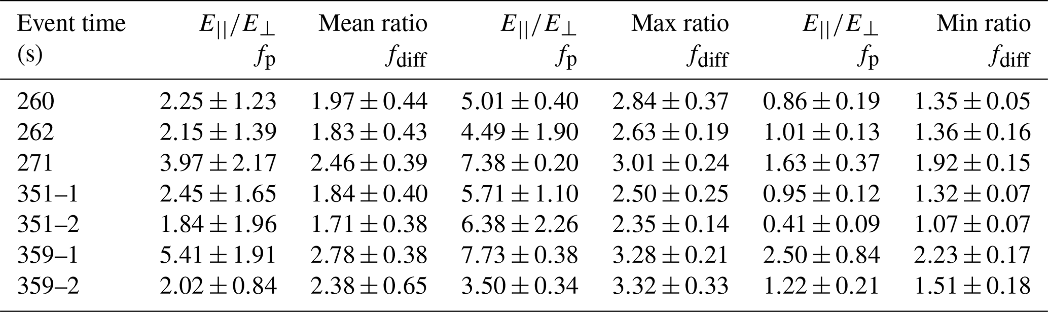
Bottom panels of each section of Fig. 4 display ratios for both the plasma line (red points) and diffuse feature (blue points) as a function of time through the five selected events. For the plasma line, the variation in this ratio is noteworthy: it seems to toggle between a fairly high ratio, around 5, and a low ratio near unity. There is no obvious feature in the spectrograms mirroring these changes in the polarization state, leading us to investigate the theoretical or instrumental reason for this unexpected result (discussed below). Because of this nonstationarity of the polarization, ratios averaged over the entire event may be misleading. Table 1 summarizes the polarization measurements of each event shown in Fig. 3. The table has seven rows because two of the events, at 351 and 359 s, have been split into two events, as indicated by the black boxes in Fig. 4d and e, because they each have a gap in the plasma line, suggesting they may be two events in close proximity. Table 1 tabulates the average ratio, which may be misleading as discussed above, the maximum ratio, defined as the average of the highest three measured ratios, and the minimum ratio, defined as the average of the lowest three measured ratios for consistency. Uncertainty estimations are based on standard deviations associated with the averages taken in obtaining each value.
Table 1Mean ratios of , maximum defined as the mean of the three largest ratios for each event, and minimum defined as the mean of the three smallest ratios for each event with their standard deviations for both the plasma line (fp) and the diffuse feature (fdiff), for Langmuir bursts defined in Figs. 2–4. Events 351 and 359 were split into two separate events because of the gap in the plasma line in the middle of the event interval.
We now use the ratios of to E⟂ to determine the wave modes and directions of propagation of the waves, by comparing the observations with theory. In order to determine what type of waves are being observed, whether they are quasi-parallel Langmuir waves or if they are oblique Z-mode waves, the ratios of the parallel to perpendicular electric field are used to determine the angle of wave propagation and compared to plasma theory. The mean ratios in Table 1 for the plasma line range from 1.8 to 5.4 and average 2.9, in approximate agreement with previous measurements which had generally lower time resolution. For example, McFadden et al. (1986) reported ratios ranging from 3–10. As noted by McFadden et al. (1986), wavelength as well as polarization can affect the measured ratio . In the case of HIBAR, electrons measured with the ESA had relatively high energy, in the range 10–20 keV. For a plasma frequency of ∼2600 kHz, this implies Langmuir waves with parallel wavelengths of ∼23–32 m would resonate with the electron distribution measured by HIBAR. Assuming that the standard electron beam Langmuir wave instability for electrons with these energies gives rise to the plasma line implies that the wavelength should exceed the probe separations, which were of order 0.3 m for the parallel measurement. The perpendicular measurement used longer boom separation, 3.0 m, but the measured ratio suggests that measurement is also in the long-wavelength regime. This means that the wave polarization should be the dominant effect determining the measured ratio for the plasma line.
McFadden et al. (1986) also point out that the perpendicular component of the wave may be underestimated in the measurement by a factor cos ϕ, where ϕ is the angle between the perpendicular electric field boom and the instantaneous perpendicular wavevector, assuming that the wave has a distinct perpendicular wavevector rather than being distributed over a range of wavevectors during the time of measurement. In the latter case, the perpendicular electric field will be underestimated by a smaller factor. These considerations raise the question of whether the observed bimodal distributions of , seemingly toggling between high values ≥5 and low values near unity, result from variations in the angle between the perpendicular boom and the wave vector projected into the plane perpendicular to B, rather than variations in the fundamental polarization of the waves. In principle, it is impossible to distinguish these two possibilities since both types of time variation of the wave vector could produce the observed ratios equally well. It is possible to infer, however, that if the angle between the perpendicular boom and the wave vector projected on the plane perpendicular to B is stationary, the mere rotation of the booms cannot explain the observed variations in (since the observed variations do not appear to repeat at the spin period).
An attempt to determine the angle of the perpendicular wavevector to the antennas' orientation results in poor fits to the observed time series of (not shown), as the observed data have zero correlation or, in some cases, the exact opposite correlation, to the expected trend based on the fit equations. The time variations in the measured suggest that either some aspect of the polarization, the ratio itself, or the angle of the E⟂ vector changes on sub-second timescales, giving rise to variations in the observed value of , or the waves are distributed over some peculiar range of angles such that the rocket spin produces this effect through variation of the angle between the boom and the projection of the electric field vector into the plane perpendicular to B. Either way, one may safely infer that exceeds k⟂ for these waves, as expected for Langmuir waves close to the plasma frequency or sufficiently oblique Z-mode waves (also known as the generalized Langmuir wave (Willes and Cairns, 2000), which is the Langmuir wave and upper-hybrid wave in the limits of parallel and perpendicular propagation, respectively, and the oblique Z modes in between).
It is worth noting, however, that Langmuir waves driven in the relatively unmagnetized solar wind by electron beams with energies of order 100 keV and above can naturally have (Graham and Cairns, 2013; Malaspina and Ergun, 2008). Because there are some observations where the perpendicular component is larger than the parallel component, it is worth determining the theoretical energies these observations would require and comparing them to the measured energies of the particles at the time of the events. Theoretically, this situation involves wave growth driven by the electron beam on or at least near the Z-mode portion of the generalized Langmuir mode, corresponding to frequencies very near and below fpe (Willes and Cairns, 2000). The relevant condition on the wavenumbers is
where k* is the wavenumber, ωpe is the electron plasma frequency, c is the speed of light, θ is the angle of the wavevector with respect to the background magnetic field, and ωce is the electron cyclotron frequency. In the HIBAR situation, where , this requires wavenumbers on the order of 0.1 m−1. Ignoring semi-relativistic and magnetization effects, the corresponding speeds are . The corresponding energies are ∼70 keV, between the energies of ∼10–100 keV considered standard for the auroral ionosphere but beyond the energy range that the electrostatic analyzer could measure. Accordingly at this time, we seek an explanation in terms of slower electron beams.
3.1 Electric field component ratios
Theory also suggests that as waves increase in frequency away from the local plasma frequency, they should become more perpendicular, decreasing the ratio of parallel to perpendicular electric field (see Fig. 6). This prediction is confirmed in this study (see Tables 1 and 2), where the ratios of the plasma lines exceed those of the diffuse feature that occurs at higher frequencies. This is true for the total average over each event interval ( for the plasma line and for the diffuse feature) and for the average max ratio between the two waves ( for the plasma line and for the diffuse feature). In the extreme case, waves near fUH reported by Samara et al. (2004) have very small ratios with an average of 0.05 (see Fig. 2 of Samara et al., 2004).
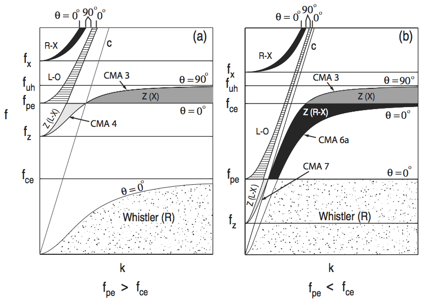
Figure 6Dispersion relations for the different wave modes for an over-dense (fpe>fce) and under-dense (fpe<fce) plasma, adapted from Benson et al. (2006). The Z-mode cutoff above the plasma frequency for an over-dense plasma increases from 0 to .
Table 2The resulting angles θ from Eq. (3) for the mean and maximum ratios defined in Table 1 for both the plasma line (θp) and diffuse feature (θdiff).
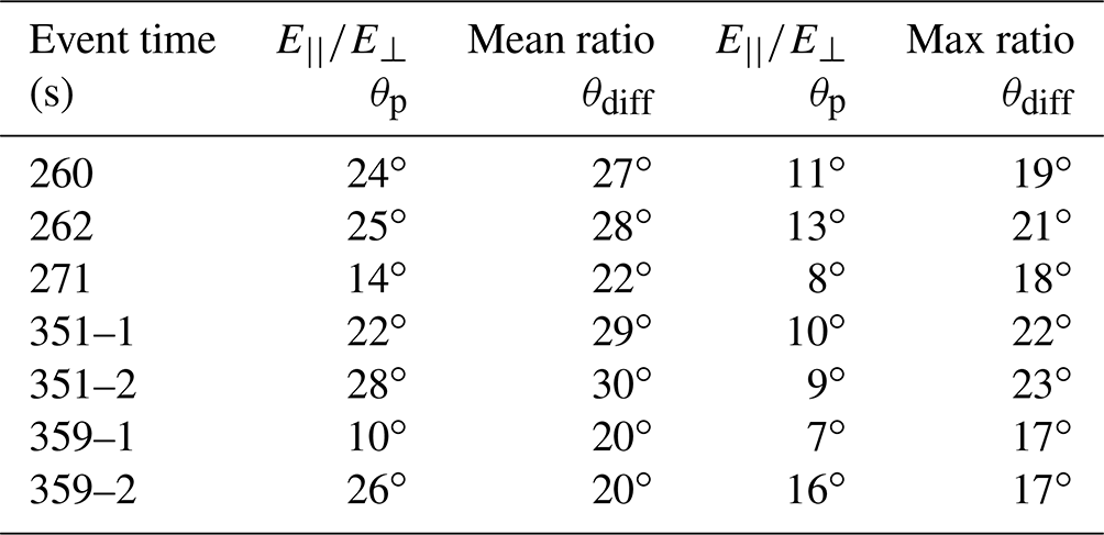
From the ratios in Table 1 the angle of wave propagation can be calculated using simple geometry by assuming the electric field amplitude ratio is proportional to the wavenumber ratio (), as expected for electrostatic waves, where the angle with respect to the magnetic field, θ, is given by
Table 2 shows calculations of these angles for both the total average ratio and the max average ratio and for both the plasma line and the diffuse feature.
The unique capability of the HIBAR mission to measure both the parallel and perpendicular components of the electric field means the propagation angles of waves with respect the background magnetic field can be compared to the expected values from plasma theory. Because these waves occur slightly above the plasma frequency cutoff in the over-dense plasma (fpe>fce), they fall into the Z-mode region (see Fig. 6 adapted from Benson et al., 2006). In this region, for waves with phase velocities less than c (speed of light), the waves can experience resonance referred to as the upper oblique resonance given by Benson et al. (2006):
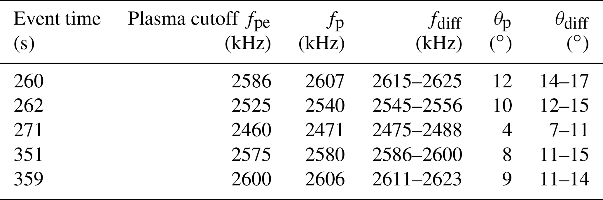
The frequency that waves can resonate in this region, Z infinity fZI, depends on the local electron plasma frequency fpe, the electron cyclotron frequency fce≈1350 kHz, and the angle that the wave propagates at with respect to the background magnetic field, θ. In the limit , fZI=fUH, and in the limit θ→0, . Table 3 lists the frequencies for the plasma cutoff (fpe), the plasma line (fp, assumed to be fZI), and the range of the diffuse feature (fdiff) for each wave burst, labeled by when they occurred in seconds post launch, along with the calculated oblique angle of the Z-infinity resonance. The angles calculated from Eq. (4) agree fairly well with the angles determined from the electric field ratios in Eq. (3). These angles agree better with the angles calculated from the average of the max power ratios than the average over all power ratios for each event for both the plasma line and diffuse feature, consistent with the nonstationary aspect of these waves. This suggests these waves are resonating at the Z-infinity resonance angle.
3.2 Nonlinear three-wave interaction
The plasma lines and corresponding diffuse features last for identical time intervals. This raises the possibility that the diffuse features are generated by wave–wave interactions of the plasma lines with lower-frequency waves. HIBAR was equipped with a very low-frequency (VLF) receiver that measured waves from 0–20 kHz, which showed a consistent whistler-mode hiss for the times when the HF waves are observed (e.g., Fig. 3). The whistler hiss ranges from 5–15 kHz and has wave electric fields on the order of tens of millivolts per meter (mV m−1). The broad range of whistler waves surrounding the rocket could interact with the plasma line to generate the broad range that the diffuse wave exhibits.
To test the plausibility of the wave–wave interaction hypothesis, a dispersion solver, Wave in Homogeneous Anisotropic Multicomponent Plasma (WHAMP; Rönnmark, 1982), was employed to calculate surfaces corresponding to the normal modes in the plasma that might participate in the wave–wave interaction: the Langmuir–upper-hybrid (UH) and the whistler–lower-hybrid (LH) surfaces. WHAMP requires user-defined input parameters for the plasma environment, including the magnetic field strength, number of particle species, and their respective densities and temperatures. Table 4 lists the parameter values used for modeling each HIBAR event. The two species used were electrons and oxygen ions, which are the dominant ions at low altitudes, and each were represented by a basic Maxwellian distribution. The densities were determined from the plasma frequency cutoff and the magnetic field from the magnetometer on board the rocket. Temperatures were taken to be 0.2 eV, typical of the auroral F region and assumed to be isotropic.
Table 4Parameters used for computing dispersion surfaces in WHAMP associated with Langmuir bursts labeled in Figs. 2–4.
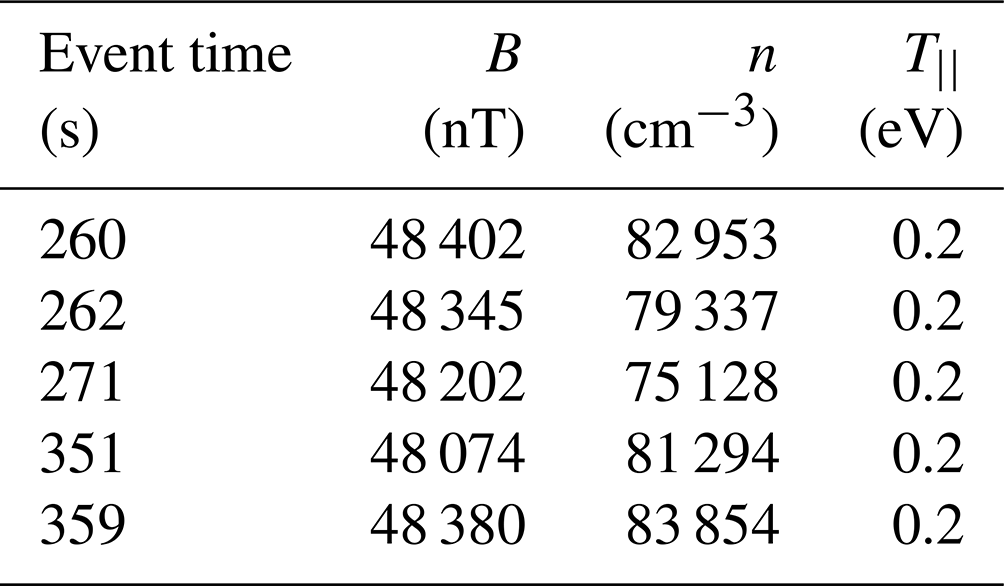
Figure 7 shows the WHAMP surfaces for each of the five events, where the x and y axes are the perpendicular and parallel wavenumbers normalized to the electron gyroradius, and the z axis is the wave frequency normalized to the electron gyrofrequency. For the Langmuir–UH surface, in the parallel wavenumber limit, the frequency equals the electron plasma frequency, and in the perpendicular limit, the frequency equals the upper-hybrid frequency. For small wavenumbers (), this surface corresponds to the Z mode (cf. Willes and Cairns, 2000). On the whistler–LH surface, in the large parallel wavenumber limit () the frequencies approach the electron cyclotron frequency. The LH surface is found at near-perpendicular propagation (). At oblique angles near parallel to B (), the surface corresponds to the whistler mode.
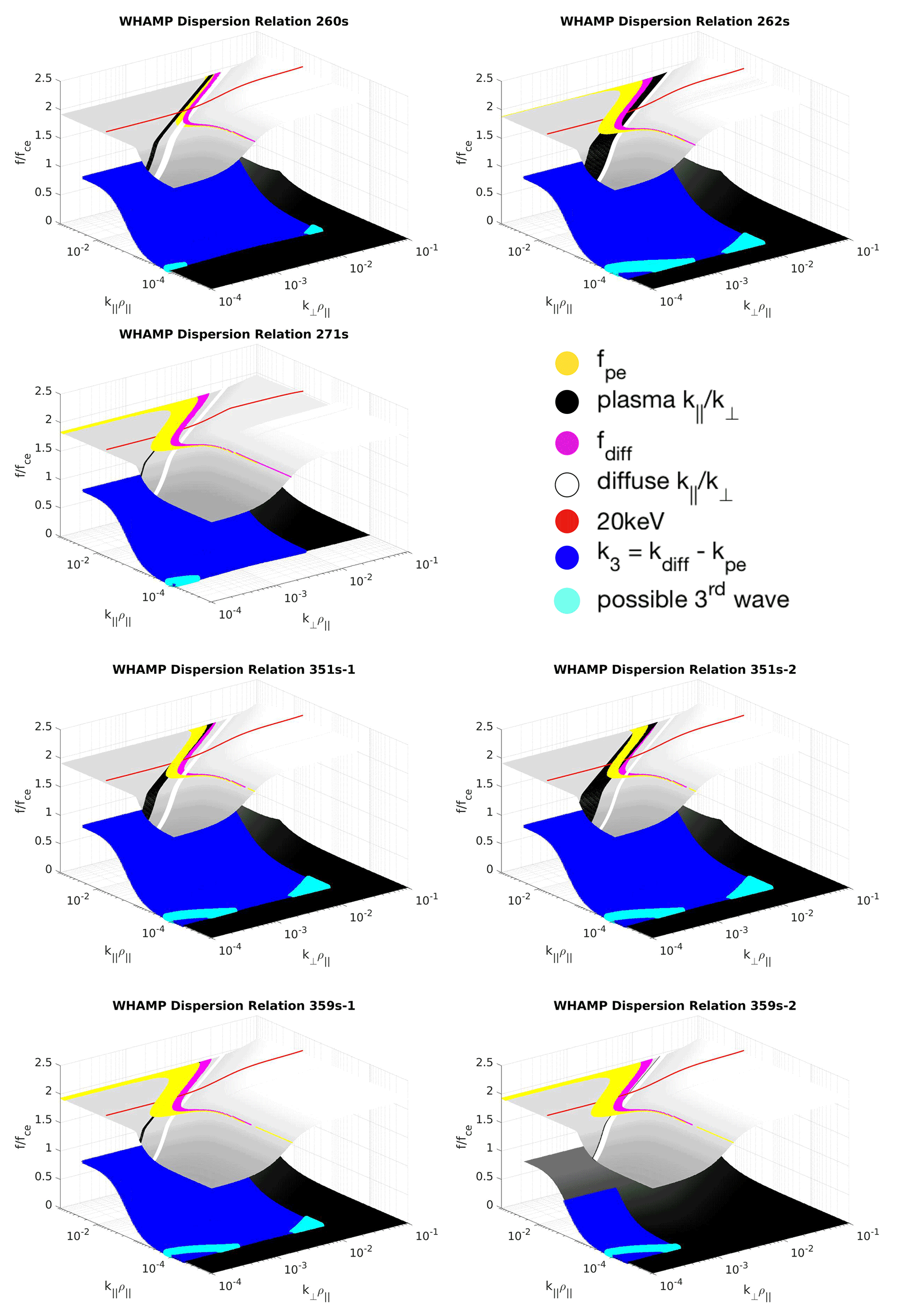
Figure 7WHAMP dispersion surfaces for Langmuir bursts labeled in Figs. 2–4, with ratios inferred from the maximum in Table 1 plotted as black for the plasma line and white for the diffuse feature. The yellow and pink areas indicate where the surface matches the frequency of the plasma line and diffuse feature, respectively. Where these intersect defines the range of possible k vectors for each wave. Assuming wave–wave interaction, kinematic equations imply a range of k vectors for the possible third wave plotted in dark blue on the whistler–LH surface and the matching frequency of the third wave plotted in light blue.
For each Langmuir–UH surface in Fig. 7, the black (white) line represents the values of inferred from the average of the maximum ratios listed in Table 1 for the plasma lines (diffuse features). The widths of these lines are determined by the standard deviations of the ratio. The corresponding plasma line and diffuse feature frequencies are plotted as patches of yellow and pink, respectively. For each plasma line and diffuse feature, where the line for intersects the patch for the observed wave frequency is the locus of allowed frequencies and wavevectors on the normal-mode surface. The red line represents where corresponds to 20 keV, the maximum electron energy observed by the electrostatic analyzer during the time of the events, via the relationship . If the plasma lines were generated by parallel Landau resonance with these high-energy electrons, then where the black plasma line ratio and yellow frequency patch intersect should be close to the condition represented by the red line. This occurs for events labeled 260s, 271s, 351s-1, 351s-2, and 359s-1.
To generate the highlighted surface sections in Fig. 7, these waves are assumed to be electrostatic; that is, the ratio of the parallel to perpendicular components of the wavevector is assumed to be equal to the ratio corresponding to electric field components. The theoretical ratios of the electric field computed by the WHAMP dispersion code for the points on the Langmuir–UH surface highlighted in Fig. 7 match the observed values (Table 1), within 10 %–25 %. This suggests that although the waves are not purely electrostatic, the values are close enough to the measured values that the assumption that is reasonable.
Assuming a nonlinear three-wave interaction is responsible for the generation of the diffuse feature, the possible third wave should be connected through the wavevector-matching condition, , which results from momentum conservation in the interaction (e.g., Tsytovich, 1970; Melrose, 1980; Cairns, 1987, 1988; Cairns and Layden, 2018; Moser et al., 2021). The wavenumbers kp and kdiff are determined by the two intersections of wavenumber ratio (black and white) and frequency matching (pink and yellow) on the Langmuir–UH surface. The dark blue patch on the whistler–LH surface in each panel of Fig. 7 represents the range of k vectors on the whistler–LH surface that satisfies this condition. The three modes must also obey the frequency-matching condition, . Light blue points within the region of possible k vectors for the third wave represent modes that also satisfy the frequency-matching condition. All events have a possible third wave that could interact with the plasma line to generate the diffuse feature. In each case, Fig. 7 suggests the third wave is well-described as a whistler/LH wave.
These waves were produced by some form of energy exchange of particles with the plasma environment, and the electron and ion data were examined to determine the source of these waves. Similar to the analysis of growth rates in Moser et al. (2021), the electron and ion distribution functions are needed to determine growth rates on the two dispersion surfaces produced by WHAMP. The measured electron distribution for the time 07:54:19.907 UT is shown in Fig. 8a, for the event labeled 260s, with a model of the high-energy electron distribution in Fig. 8b produced by the WHAMP parameters: temperature, density, magnetic field strength, drift velocity, and anisotropy. The x axis represents the parallel velocity, where the positive axis is along the background magnetic field and the negative axis is anti-parallel to the magnetic field. The y axis represents the velocity perpendicular to the background magnetic field. The high-energy electrons, while not the most prominent feature in the electron distribution, were used to model the distribution because Eq. (2) suggests these waves are produced by particles with higher energies. It should be noted that the electron ESA could only measure electrons with energies below 20 keV, which limits the range of electron energies that can be modeled.
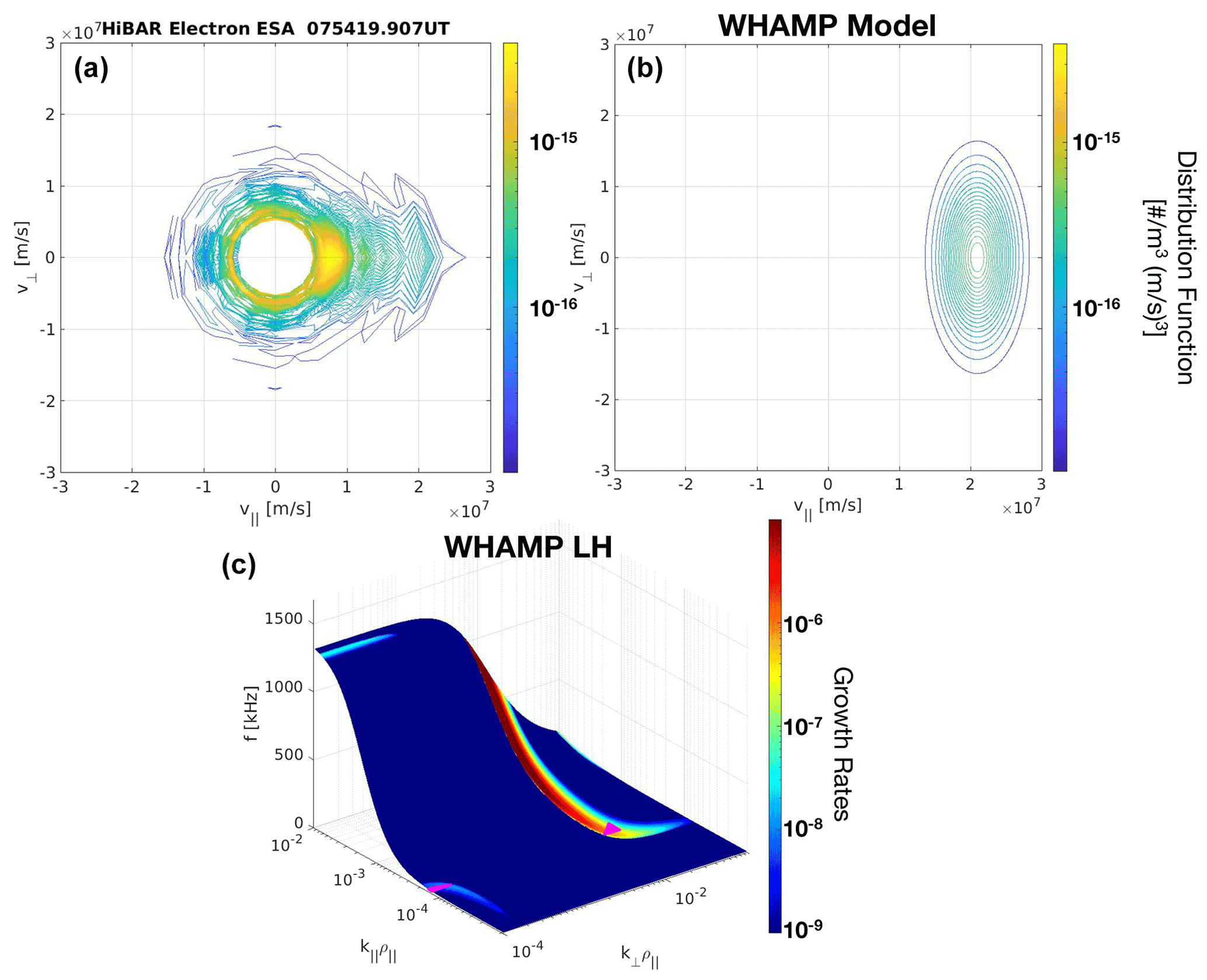
Figure 8Measured electron distribution function from HIBAR's electron ESA data at 07:54:19.907 (a) and model of the high-energy beam seen in the measured distribution using a drifting Maxwellian (b). Panel (c) shows the growth rates on the whistler/LH-mode surface produced by the model WHAMP distribution, along with the frequency- and wavenumber-matching conditions for the event labeled 260s in pink. The Langmuir/Z-mode surface showed no growth on the surface from this distribution.
Figure 8c shows the whistler–LH-mode surface produced in WHAMP with growth rates from the model distribution in Fig. 8b for the event labeled 260s. The model distribution has a parallel temperature eV, a density n=1 cm−3, a magnetic field B=48 402.0 nT, a drift velocity , and an anisotropy ratio of . There are two areas of growth that are of interest, at low k⟂ and high k⟂, where the frequency- and wavenumber-matching conditions are met. At low k⟂ the growth rate is Hz, smaller than the growth rates at higher k⟂ of Hz, but both are too low to likely produce these waves. However, the true unstable distributions may not be captured with the particle instruments, even with proper energy range and resolution, because unstable distributions rapidly stabilize. So while the growth rates with the observed distribution are low, they show that growth should occur and could increase to nonlinear levels with a more suitable electron distribution. The areas of larger growth at higher frequencies near on the whistler-mode surface are potentially generating the whistler-mode waves observed in the HF spectra at frequencies between about 50 and 350 kHz. The model electron distribution in Fig. 8 was also used to generate the Langmuir–Z-mode surface (not shown) and found to produce no instabilities at frequencies and wavenumbers that correspond to the modes in Fig. 7.
Other possible sources of free energy are electrons above 20 and below 60 eV as well as the ions. Because the high- and low-energy electrons were not measured, they could not be modeled with WHAMP to find unstable features. As stated above, the instability that would be the source of the observed Langmuir waves may result from higher-energy electrons than those that were measured. The ions were measured from 80 eV to 20 keV with a time resolution of 45 ms. In a similar analysis to that described above, the observed ion ring-like distribution at 09:54:19.920 UT was modeled using the WHAMP parameters, and growth rates on the whistler/LH modes were analyzed. The resulting model produced low growth rates on the surface ( Hz) but at wavevectors and frequencies that do not match those seen in Fig. 7. Therefore, the ions are unlikely to be the source of these waves.
Another test of plausibility for a wave–wave interaction is to compare the electric energy density of the different waves to the thermal plasma energy density. The electric energy density, , for the plasma line is J m−3 and for the diffuse band is J m−3, 100 times smaller than that of the plasma line. The whistler/LH-mode waves (likely dominated by whistler-mode hiss) has an electric energy density of approximately 10−16 J m−3. In comparison the plasma's thermal energy density is J m−3, where cm−3 is the plasma number density and kBT=0.2 eV is the typical auroral F-region temperature assumed for all events. The ratio of the electric to the thermal energy densities is for the plasma line, 10−14 for the diffuse band, and 10−7 for the whistler/LH-mode hiss. Because the diffuse feature is much weaker than the plasma line and the whistler/LH-mode hiss, it suggests that the diffuse feature is a product of a wave–wave coalescence process () between the two others, the plasma line (L) and whistler/LH-mode hiss (W). The whistler/LH-mode energy density being much larger than the other two suggests that this is the primary driving wave, and the plasma line Langmuir waves are secondary, with the diffuse band being a product wave.
Incidentally, Akbari et al. (2013) observed double-peaked plasma lines in incoherent scatter radar data associated with strongly turbulent Langmuir cavitons. Although there is a superficial resemblance to the double-peaked plasma frequency spectra reported here, the extremely low ratio of electric to thermal energies in this case preclude an association with cavitons.
A more quantitative analysis is to examine the ratio of wave occupation numbers for these waves. The electric energy density is related to the plasmon occupation number through
where Ri(k) is the ratio of the electric to total energy, Ni(k) is the occupation number, and the volume integral is over the relevant region of wavevector space for a participating set of waves (e.g for the plasma line). The ratios Ri(k), as determined by WHAMP, are approximately for both the plasma line and diffuse feature and for the whistler-mode hiss. For the plasma line, combining this value of Ri(k) with the observed electric energy density leads to a total energy density of approximately J m−3. The same procedure leads to total energy densities of and J m−3 for the diffuse waves and the VLF whistlers, respectively.
Assuming the occupation numbers are the same for each wave mode, Eq. (5) can be rearranged and the ratios of occupation numbers determined to be
The difficulty with solving this equation is determining the range of wavevectors that the modes occupy. To get a rough estimate of the ranges, the WHAMP surfaces are examined to determine possible ranges of wavenumbers for the observed waves and get an idea for the ratio of the occupation numbers. For the plasma line and diffuse feature, the broad range of wavevectors is –10−2 and –. For the whistler/LH mode, the wavevector range –10−2 and –, where m. This covers the square patch of the surface where the different wave modes occur that match the conditions in Fig. 7. Choosing these ranges in the wavevector integrals in Eq. (7) leads approximately to
Following a similar derivation for the time rate of change of the occupation numbers as in Moser et al. (2021), Cairns (1988), and Melrose (1980), among others, we can show that at saturation (when the rates of change of NL and NW are zero, ignoring linear growth and damping) the relationship of the whistler/LH-mode occupation number to the Langmuir wave occupation numbers for the coalescence process is
For each plasmon lost from the whistler/LH mode and the plasma line as the coalescence proceeds, the diffuse mode gains one plasmon. From Eq. (9) the process saturates when
This leads to a very small ratio of the Langmuir-mode occupation numbers to the whistler/LH mode, with when NL≪NW, which we have shown is the case from Eq. (7) for the observations.
Based on the foregoing observations and theoretical analyses it appears plausible that the diffuse band is formed by the nonlinear coalescence of whistler/LH-mode waves W near the LH frequency with Langmuir waves L. The presumption is that the L and W waves are produced by distinct linear instabilities, most likely driven by an electron beam and/or by temperature anisotropies.
The HIBAR rocket was launched into active pre-midnight aurora and observed seven short duration bursts of Langmuir waves above the local plasma frequency at altitudes from 364–377 km. Of these seven events, five consisted of a plasma line at frequencies ranging from 2470–2610 kHz with an associated diffuse feature occurring 5–15 kHz above this line. Independent measurements of both the parallel and perpendicular components of the electric field showed that the plasma lines typically have , and the diffuse features have . These results are consistent with previous measurements of Langmuir wave components and are in line with theory, where waves in an over-dense plasma above the plasma frequency experience Z-infinity resonance at angles with respect to the background magnetic field defined by Eq. (4). Using this equation with the plasma line and diffuse band frequencies shows that these waves would propagate at angles between 5–20∘, which are comparable with the propagation angles produced by the ratio values using Eq. (3).
WHAMP was used to identify the Langmuir–Z and whistler–LH surfaces where the plasma line and diffuse feature's wave modes would occur. The values are also consistent with the Langmuir–Z surface at moderately oblique angles. Wavevector and frequency conservation for a three-wave process involving the plasma line and diffuse band regions of the dispersion surface is consistent with the third wave being on the whistler/LH surface close to perpendicular propagation and with frequencies close to the LH frequency. The electron and ion data were used to determine instabilities on the LH surface and determined that the high-energy electrons are the more likely source of these waves. The observed electric field energy densities of the whistler/LH waves are large enough, in comparison to the thermal energy density, for a nonlinear process to be viable. The wave energy densities decrease from the whistler/LH waves to the plasma line Langmuir waves to the diffuse band. Comparison of the different wave-mode occupation numbers suggests the most plausible explanation is the coalescence of whistler/LH waves W with Langmuir waves L from the plasma line to produce the diffuse band of Langmuir waves L′ via the process . Both the W and L waves are believed to be produced by distinct linear instabilities.
This is similar to the process in Staciewicz et al. (1996), where observation of modulated Langmuir waves suggested these waves were produced through either parametric decay of the primary Langmuir wave into a LH wave and secondary Langmuir waves via the process or through the scattering of Langmuir waves off preexisting LH waves via the process , itself obviously a coalescence process. Bonnell at al. (1997) also presented a similar study of modulated Langmuir waves thought to be produced scattering off electrostatic whistler/LH waves and showed this was the more likely process than the decay process in their situation. The observations presented here seem to be a similar process to these two studies, of a Langmuir/Z-mode wave coalescing with or scattering off of the whistler/LH but here with the Langmuir/Z-mode waves having significantly weaker amplitudes.
Data are available to the public at https://phi.physics.uiowa.edu/science/tau/data0/rocket/HIBAR_36200/ (Bounds, 2021).
JL was the PI for the HIBAR mission. JL and CM interpreted the data and experiment. CM wrote the codes and performed the data analysis. IHC contributed the theoretical analysis, and all authors contributed to the interpretation of the results. CM wrote the manuscript with contributions from all authors.
The contact author has declared that neither they nor their co-authors have any competing interests.
Publisher's note: Copernicus Publications remains neutral with regard to jurisdictional claims in published maps and institutional affiliations.
Thanks are expressed to the team at Wallops Flight Facility and NASA for supporting the HIBAR payload and launch, as well as engineer Hank Harjes and NASA engineer Bill Payne for instrumentation support. Authors also thank Marilia Samara, Connor Feltman, and Scott Bounds for discussions and support. Research at Dartmouth College was supported by NASA grant NNX17AF92G.
This research has been supported by the National Aeronautics and Space Administration (grant no. NNX17AF92G).
This paper was edited by Igo Paulino and reviewed by Abraham C. L. Chian and Peter Yoon.
Akbari, H., Semeter, J. L., Nicolls, M. J., Broughton, M., and LaBelle, J. W.: Localization of auroral Langmuir turbulence in thin layers, J. Geophys. Res.-Space, 118, 3576–3583, 2013.
Akbari, H., Labelle, J. W., and Newman, D. L.: Langmuir Turbulence in the Auroral Ionosphere: Origins and Effects, Frontiers in Astronomy and Space Sciences, 7, 116, 2021.
Beghin, C., Rauch, J. L., and Bosqued, J. M.: Electrostatic plasma waves and HF auroral hiss generated at low altitude, J. Geophys. Res.-Space, 94, 1359–1378, 1989.
Benson, R. F., Webb, P. A., Green, J. L., Carpenter, D. L., Sonwalkar, V. S., James, H. G., and Reinisch, B. W.: Active wave experiments in space plasmas: The Z mode, in: Geospace Electromagnetic Waves and Radiation, Springer, 3–35, ISBN 978-3-540-33203-9, 2006.
Boehm, M. H., Carlson, C. W., McFadden, J. P., Clemmons, J. H., and Mozer, F. S.: High-resolution sounding rocket observations of large-amplitude Alfvén waves, J. Geophys. Res.-Space, 95, 12157–12171, 1990.
Bonnell, J., Kintner, P., Wahlund, J.-E., and Holtet, J. A.: Modulated langmuir waves: observations from freja and SCIFER, J. Geophys. Res.-Space, 102, 17233–17240, 1997.
Bounds, S.: Data from the HIBAR 32600 sounding rocket mission [data set], https://phi.physics.uiowa.edu/science/tau/data0/rocket/HIBAR_36200/, last access: October 2021.
Cairns, I. H.: Third and higher harmonic plasma emission due to Raman scattering, J. Plasma Phys., 38, 199–208, 1987.
Cairns, I. H.: A theory for the radiation at the third to fifth harmonics of the plasma frequency upstream from the Earth's bow shock, J. Geophys. Res.-Space, 93, 858–866, 1988.
Cairns, I. H. and Layden, A.: Kinematics of electrostatic 3-wave decay of generalized Langmuir waves in magnetized plasmas, Phys. Plasmas, 25, 082309, https://doi.org/10.1063/1.5037300, 2018.
Chian, A. C.-L., Lopes, S. R., and Alves, M. V.: Generation of auroral whistler-mode radiation via nonlinear coupling of Langmuir waves and Alfvén waves, Astron. Astrophys., 290, L13–L16, 1994.
Colpitts, C. A. and LaBelle, J.: Mode identification of whistler mode, Z-mode, and Langmuir/Upper Hybrid mode waves observed in an auroral sounding rocket experiment, J. Geophys. Res.-Space, 113, A04306, https://doi.org/10.1029/2007JA012325, 2008.
Dombrowski, M. P., LaBelle, J., Rowland, D. E., Pfaff, R. F., and Kletzing, C. A.: Interpretation of vector electric field measurements of bursty Langmuir waves in the cusp, J. Geophys. Res.-Space, 117, A09209, https://doi.org/10.102A09209, 2012.
Ergun, R. E., Carlson, C. W., McFadden, J. P., Clemmons, J. H., and Boehm, M. H.: Langmuir wave growth and electron bunching: Results from a wave-particle correlator, J. Geophys. Res.-Space, 96, 225–238, 1991.
Ergun, R. E., Carlson, C. W., McFadden, J. P., Mozer, F. S., Muschietti, L., Roth, I., and Strangeway, R. J.: Debye-scale plasma structures associated with magnetic-field-aligned electric fields, Phys. Rev. Lett., 81, 826, 1998.
Ergun, R. E., Malaspina, D. M., Cairns, I. H., Goldman, M. V., Newman, D. L., Robinson, P. A., Eriksson, S., Bougeret, J. L., Briand, C., Bale, S. D., Cattell, C. A., Kellogg, P. J., and Kaiser, M. L.: Eigenmode structure in solar-wind Langmuir waves, Phys. Rev. Lett., 101, 051101, https://doi.org/10.1103/PhysRevLett.101.051101, 2008.
Graham, D. B. and Cairns, I. H.: Electrostatic decay of Langmuir/z-mode waves in type III solar radio bursts, J. Geophys. Res.-Space, 118, 3968–3984, 2013.
Khotyaintsev, Y., Lizunov, G., and Stasiewicz, K.: Langmuir wave structures registered by FREJA: analysis and modeling, Adv. Space Res., 28, 1649–1654, 2001.
Kintner, P. M., Bonnell, J., Powell, S., Wahlund, J.-E., and Holback, B.: First results from the Freja HF snapshot receiver, Geophys. Res. Lett., 22, 287–290, 1995.
LaBelle, J. and Treumann, R. A.: Auroral radio emissions, 1. Hisses, roars, and bursts, Space Sci. Rev., 101, 295–440, 2002.
LaBelle, J., Cairns, I. H., and Kletzing, C. A.: Electric field statistics and modulation characteristics of bursty Langmuir waves observed in the cusp, J. Geophys. Res.-Space, 115, A10317, https://doi.org/10.1029/2010JA015277, 2010.
Lizunov, G. V., Khotyaintsev, Y., and Stasiewicz, K.: Parametric decay to lower hybrid waves as a source of modulated Langmuir waves in the topside ionosphere, J. Geophys. Res.-Space, 106, 24755–24763, 2001.
Lopes, S. R. and Chian, A. C.-L.: A coherent nonlinear theory of auroral Langmuir-Alfven-whistler (LAW) events in the planetary magnetosphere, Astron. Astrophys., 305, 669, 1996.
Lund, E. J. and LaBelle, J.: On the generation and propagation of auroral electromagnetic ion cyclotron waves, J. Geophys. Res.-Space, 102, 17241–17253, 1997.
Malaspina, D. M. and Ergun, R. E.: Observations of three-dimensional Langmuir wave structure, J. Geophys. Res.-Space, 113, A12108, https://doi.org/10.1029/2008JA013656, 2008.
McAdams, K. L. and LaBelle, J.: Narrowband structure in HF waves above the electron plasma frequency in the auroral ionosphere, Geophys. Res. Lett., 26, 1825–1828, 1999.
McAdams, K. L., LaBelle, J., Trimpi, M. L., Kintner, P. M., and Arnoldy, R. A.: Rocket observations of banded structure in waves near the Langmuir frequency in the auroral ionosphere, J. Geophys. Res.-Space, 104, 28109–28122, 1999.
McAdams, K. L., Ergun, R. E., and LaBelle, J.: HF chirps: Eigenmode trapping in density depletions, Geophys. Res. Lett., 27, 321–324, 2000.
McFadden, J. P., Carlson, C. W., and Boehm, M. H.: High-frequency waves generated by auroral electrons, J. Geophys. Res.-Space, 91, 12079–12088, 1986.
Melrose, D. B.: Plasma Astrophysics, Vol. II, Gordon and Breach Science Publisher Inc., ISBN 0-667-03490-3. 1980.
Moser, C., LaBelle, J., Roglans, R., Bonnell, J. W., Cairns, I. H., Feltman, C., Kletzing, C. A., Bounds, S., Sawyer, R. P., and Fuselier, S. A.: Modulated Upper-Hybrid Waves Coincident with Lower-Hybrid Waves in the Cusp, J. Geophys. Res.-Space, 126, e2021JA029590, https://doi.org/10.1029/2021JA029590, 2021.
Rönnmark, K.: WHAMP-Waves in homogeneous, anisotropic, multicomponent plasmas, Tech. rep., Kiruna Geofysiska Inst. (Sweden), KGI Report No. 179, ISSN 0347-6405, 1982.
Samara, M. and LaBelle, J.: Structured waves near the plasma frequency observed in three auroral rocket flights, Ann. Geophys., 24, 2911–2919, https://doi.org/10.5194/angeo-24-2911-2006, 2006.
Samara, M., LaBelle, J., Kletzing, C. A., and Bounds, S. R.: Rocket observations of structured upper hybrid waves at fuh=2fce, Geophys. Res. Lett., 31, L22804, https://doi.org/10.1029/2004GL021043, 2004.
Schamel, H., Mandal, D., and Sharma, D.: Diversity of solitary electron holes operating with non-perturbative trapping, Phys. Plasmas, 27, 062302, https://doi.org/10.1063/5.0007941, 2020.
Stasiewicz, K., Holback, B., Krasnoselskikh, V., Boehm, M., Boström, R., and Kintner, P. M.: Parametric instabilities of Langmuir waves observed by Freja, J. Geophys. Res.-Space, 101, 21515–21525, 1996.
Tsytovich, V.: Nonlinear effects in plasma, Plenum Press, New York, ISBN 987-1-4684-1788-3, 1970.
Willes, A. J. and Cairns, I. H.: Generalized Langmuir waves in magnetized kinetic plasmas, Phys. Plasmas, 7, 3167–3180, 2000.