A case study of a ducted gravity wave event over northern Germany using simultaneous airglow imaging and wind-field observations

An intriguing and rare gravity wave event was recorded on the night of 25 April 2017 using a multiwavelength all-sky airglow imager over northern Germany. The airglow imaging observations at multiple altitudes in the mesosphere and lower thermosphere region reveal that a prominent upward-propagating wave structure appeared in O(¹S) and O₂ airglow images. However, the same wave structure was observed to be very faint in OH airglow images, despite OH being usually one of the brightest airglow emissions. In order to investigate this rare phenomenon, the altitude profile of the vertical wavenumber was derived based on colocated meteor radar wind-field and SABER temperature profiles close to the event location. The results indicate the presence of a thermal duct layer in the altitude range of 85–91 km in the southwest region of Kühlungsborn, Germany. Utilizing these instrumental data sets, we present evidence to show how a leaky duct layer partially inhibited the wave progression in the OH airglow emission layer. The coincidental appearance of this duct layer is responsible for the observed faint wave front in the OH airglow images compared O(¹S) and O₂ airglow images during the course of the night over northern Germany.

1 Introduction

Multiwavelength nighttime all-sky airglow imaging has become a widely used technique to retrieve valuable information of atmospheric gravity waves (GWs) as well as the dynamics of the mesosphere and lower thermosphere (MLT) region. GWs play a key role in the upper atmospheric dynamics because of their inherent properties of transferring momentum and energy from lower atmospheric regions to the middle and upper atmosphere (Fritts and Alexander, 2003). However, the ducting inhibits the vertical propagation of GWs and confines the major flow of wave energy and momentum to a rather limited altitude region (Chimonas and Hines, 1986). The earlier imaging studies using airglow emissions originating in the MLT region revealed different types of dynamical events like quasi-monochromatic GWs, ripples, and mesospheric fronts (Taylor et al., 1995; Walterscheid et al., 1999; Hecht et al., 2001; Smith et al., 2003; Makhlouf et al., 1995; Bageston et al., 2011; Lakshmi Narayanan et al., 2012; Sarkhel et al., 2012, 2015a, b, 2019; Hozumi et al., 2019; Mondal et al., 2021; Guharay et al., 2022).

The characteristics and morphology of gravity wave events have been investigated for decades. Depending upon the characteristics and background conditions, the evolution of GWs in the atmosphere can be rather different. Large-scale waves (several tens of kilometers horizontal wavelength) can easily reach to the MLT region depending on their phase velocity compared to the background mean flow, whereas small-scale (a few tens of kilometers horizontal wavelength) waves are more susceptible to thermal and Doppler ducting (Walterscheid et al., 1999). The evolution of GWs and their interaction with the mean flow have been extensively studied using the linear theory of GWs. The waves can exert a significant amount of drag in the mean flow of the atmosphere and thereby play an important role in the middle atmospheric circulation. In addition, waves can break due to occurrence of neutral instabilities into and generate secondary waves or ripple type structures (Vadas et al., 2018; Becker and Vadas, 2018; Heale et al., 2020). Large-scale GWs can interact with the mean flow and generate one of the most puzzling mesospheric phenomena known as the mesospheric fronts (Dewan and Picard, 1998, 2001; Smith et al., 2005, and references therein). Mesospheric fronts can also propagate over long horizontal distances and therefore act as an efficient mechanism for transferring energy and momentum over long ranges with negligible energy loss in the atmosphere (Medeiros et al., 2018). Therefore, GW propagation through a region of thermal or Doppler ducting can explain some of the properties of mesospheric fronts like the long-distance horizontal propagation.

The inhomogeneities in the temperature and wind field are responsible for the static/convective and dynamic instabilities, respectively, in the atmosphere, which affect the wave propagation. In particular, vertical gradients in temperature and wind field give rise to numerous interesting phenomena like wave reflection, wave ducts, or waveguides in the MLT region. GWs can be ducted in a region where the vertical wavenumber (m) of the GWs is real (m² > 0), and the region is situated between two atmospheric altitude regions of imaginary vertical wavenumber (m² < 0). Once the GW falls into this ducted region, it gets trapped because of repeated reflection from the bottom and upper layer (reflectance layers). However, the wave can freely propagate in a horizontal direction. If there is a reflection layer at a certain height, GWs can get reflected from this layer. The ducted wave is called thermally ducted or Doppler ducted (or both) according to whether m² < 0 arises predominantly from the temperature gradient or the vertical shear of the horizontal wind (Walterscheid et al., 1999). A thermal duct is isotropic and will support ducted wave activity with any orientation, whereas a Doppler duct is very sensitive to the wave orientation (Fritts and Yuan, 1989). In this paper, we present a case study of a mesospheric wave structure using a multiwavelength all-sky airglow imager and simultaneous measurements of 2D horizontally resolved wind field in the MLT region over northern Germany. Here, we present a first case study with the MMARIA (Multi-static, Multifrequency Agile Radar for Investigations of the Atmosphere) meteor radar network in Germany (Stober an Chau, 2015; Stober et al., 2018) and colocated all-sky airglow imaging observations combining the available horizontally resolved wind and airglow information to infer the intrinsic GW parameters.

2 Experimental techniques

A multiwavelength all-sky airglow imager was procured from Boston University, USA, and installed at Leibniz Institute for Atmospheric Physics, Kühlungsborn (54.11^∘ N, 11.77^∘ E), Germany. The imager has been operating since November 2016. The imager design is similar to an all-sky imager that is being operated at Padua Observatory, Asiago (Smith et al., 2017). The details of the imager and a few results are available in Vargas et al. (2021). The imager features an Andor back-illuminated bare-CCD camera with 1024 × 1024 pixels resolution and a 16 mm fish-eye lens that allows for a maximum field of view (FOV) of 180^∘. On the night of 25 April 2017, the images were binned 2 × 2 (in real time) in order to achieve better signal-to-noise ratio. The system is equipped with a temperature-controlled filter wheel that can record OH broadband emission (695–1050 nm) with a notch at 866.0 nm, Na emission (589.3 nm), O₂ emission (866.0 nm) and O(¹S) emission (557.7 nm) in the MLT region. The cycling of the filter wheel operation (with exposure time) is as follows: OH (27 s) ⇒ 866.0 nm (134 s) ⇒ 557.7 nm (260 s) ⇒ 589.3 nm (263 s). Based on rocket measurements, it has been reported that these airglow emissions originate from layers of 8–11 km full width at half maxima (FWHM) or thickness with centroid heights of around 86, 91, 94, and 97 km (Watanabe et al., 1981; Ogawa et al., 1987; Baker and Stair, 1988; Gobbi et al., 1992; Mende et al., 1993; Hedin et al., 2009). In addition, the imager also records thermospheric emission O(¹D) (630.0 nm) from ∼ 250 km altitude with around 40 km layer thickness (Sobral et al., 1992). The imager is also equipped with a background filter in which the nightglow is minimal. This filter has a central wavelength of 605.0 nm and is used for photometric calibration of the images. In our investigation, we have used only emission originating from the MLT region. The bandwidth of the 589.3, 866.0, and 557.7 nm filters is 2.0 nm, whereas the OH filter is a broadband (695–1050 nm) filter with a notch at 866.0 nm in order to exclude the O₂ emission line completely. Hence, there is no contamination of OH broadband emission from other mesospheric lines (557.7 and 589.3 nm). The nearest lines of OH (X²Π) are at P1(6) and R(7,3) (854.9 and 877.1 nm, respectively) that are quite far off from the O₂ emission line (866.0 nm) (Osterbrock et al., 1996). In addition, the wave signatures in the OH (when detected) and O₂ images differed in both morphology and phase. Hence, we are confident that no significant broadband OH occurred within the 866.0 nm filter bandwidth. The integration times for the 589.3, 866.0, and 557.7 nm images were 120 and 15 s for the OH filter.

The second data set used in this study is based on a meteor radar network operated in northern Germany known as MMARIA (Multi-static, Multi-frequency Agile Radar for Investigations of the Atmosphere) (Stober and Chau, 2015). In this study, we used the Juliusruh meteor radar (54.6^∘ N, 13.3^∘ E) (e.g., Hoffmann et al., 2010) with a transmit power of 30 kW operated at 32.55 MHz, the Collm meteor radar (51.1^∘ N, 13.0^∘ E) (e.g., Jacobi et al., 2007) with a transmit power of 15 kW operated at 36.2 MHz, and three multistatic passive systems installed at Kühlungsborn and Juliusruh. The bistatic meteor detections from transmissions originating in Juliusruh and Collm are received interferometrically at 32.55 and 36.2 MHz, respectively. The horizontally resolved 2D wind field is based on the packed retrieval algorithm presented in Stober et al. (2018). Further, we restricted the domain size to be slightly larger than the field of view of the airglow imager. The temporal resolution of the 2D wind field was 1 h with a vertical resolution of 2 km at altitudes between 80 and 100 km. The spatial grid for horizontally resolved winds is chosen to be 30 km × 30 km parallel to the Earth's surface. All coordinates and radial velocities are corrected for projection errors using the WGS84 model (National Imagery and Mapping Agency, 2000). An initial validation of the 2D wind-field retrievals and more details of the technique can be found in Stober et al. (2018, 2021).

Another data set is the altitude profile of temperature that has been obtained from the SABER instrument aboard the TIMED satellite (data source: http://saber.gats-inc.com, last access: 15 January 2022; v2.0; level 2A). The retrieval of the ambient temperature at a given altitude is carried out using 15 µm emission from CO₂ molecules in the atmosphere. The location of the SABER measurement is less than 150 km from the southwest corner of the imager FOV from where the wave entered. The uncertainty in the SABER temperature retrievals is around ±3 K at 80 km, ±8 K at 90 km, ±1–2 K below 95 km, and ±4 K at 100 km in the midlatitudes (García-Comas et al., 2008).

Figure 1 reveals the map of northern Europe where it shows the location of the multiwavelength airglow imager at Kühlungsborn, the Collm and Juliusruh meteor radar, and the receiver stations at Juliusruh and Kühlungsborn. The yellow box is the maximum horizontal coverage of the airglow imager in the MLT region. The red asterisks are the SABER temperature measurement locations. It is to be noted here that SABER 1 measurement location is quite far from the imager field of coverage, whereas the measurement location of SABER 2 is close to the edge of the horizontal coverage of the airglow imager.

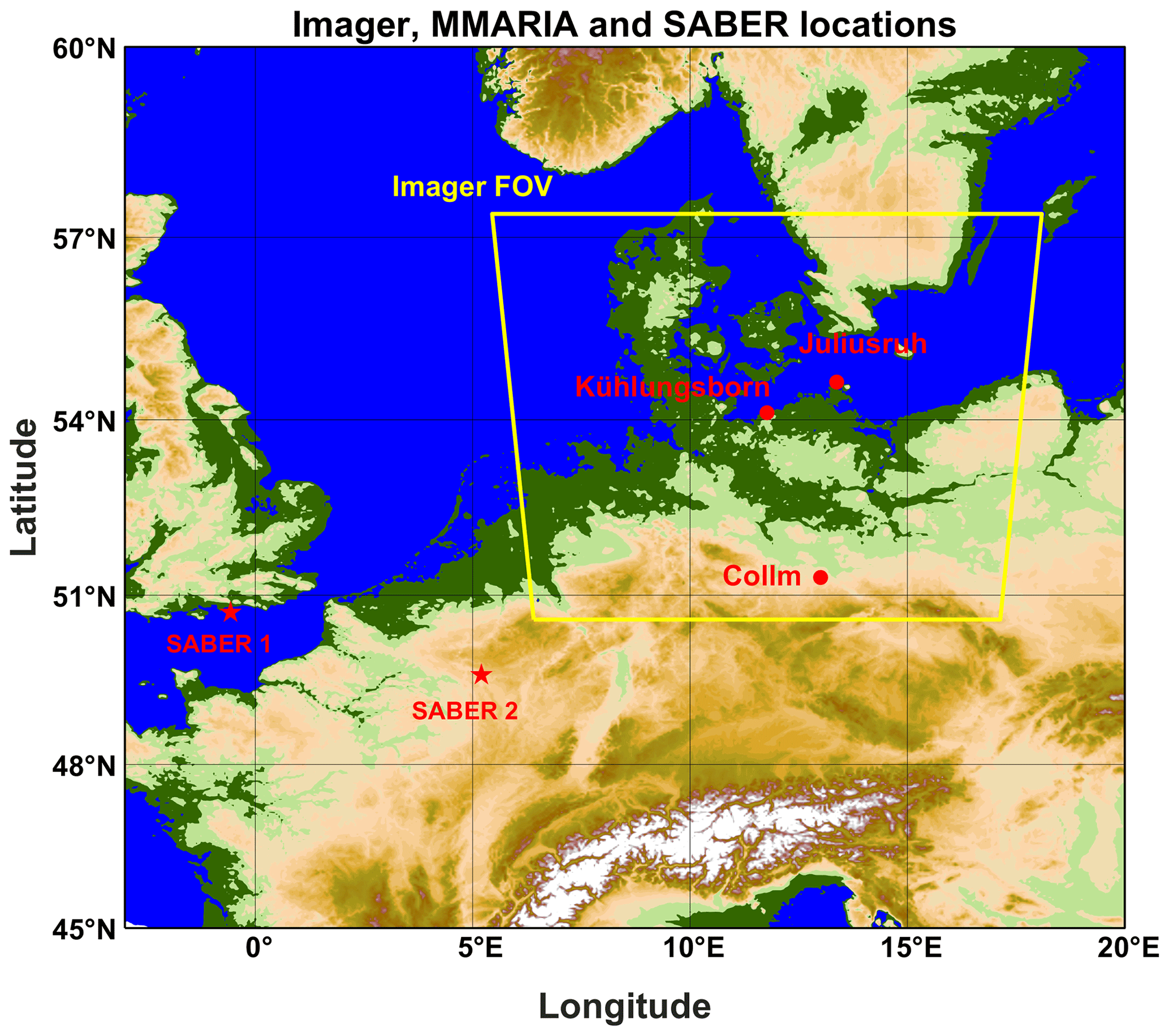
Figure 1 The map of northern Europe where it shows the location of the multiwavelength airglow imager at Kühlungsborn, MMARIA transmitter stations (Collm and Juliusruh), and receiver stations (Juliusruh and Kühlungsborn). The map has been generated from ETOPO1 1 Arc-Minute Global Relief Model (Amante and Eakins, 2009). The yellow box is the maximum horizontal coverage of the airglow imager in the MLT region. The red asterisks show the SABER temperature measurement locations.

3 Data analyses

In order to retrieve scientific information, the raw images need to be processed. The standard methods of image processing including geospatial calibration, star removal, and unwarping are available in the literature (Garcia et al., 1997; Mondal et al., 2019, and references therein). In most situations, the unwarped images are noisy and not very clear. It can be verified from Figs. 2–5a–f that the unwarped images are noisy for all the airglow filters. For the derivation of the wavelength, apparent periodicity, and phase velocity of the perturbation from the intensity fluctuation, the unfiltered unwarped images may not be suitable. Therefore, in order to enhance the intensity perturbation by suppressing the noise, the 2D fast Fourier transform (FFT) filtering techniques have been adopted from Mondal et al. (2019). In this filtering technique, Savitzky–Golay (SG) and Gaussian window sizes are crucial. These window sizes are optimized for each airglow emission filter, which is discussed in Mondal et al. (2019) in detail. In the present case, the window size of SG filter is taken as 400 pixels for OH, 350 pixels for 589.3 nm, and 300 pixels for 866.0 nm, 300 pixels for 557.7 nm filter. On the other hand, the Gaussian filter has standard deviation (σ) of 20 pixels for OH, 20 pixels for 589.3 nm, and 15 pixels for 866.0 nm, 15 pixels for 557.7 nm filter. Here, 1 pixel on the airglow images is nearly equal to 1.16 km. It may be noted that the wave-like features in the filtered unwarped images are enhanced (shown in panels g–l of Figs. 2–5). These filtered unwarped images are utilized to derive the apparent phase velocity and horizontal wavelength of the wave structure. In order to proceed further, a line is overlaid along the direction of propagation for the particular number of consecutive images in which the wave structure has been detected visually. This arrow (shown in panels g–l of Figs. 2–5) represents the wave vector of the structure. From the intensity variation along the line of propagation, the apparent phase velocity and horizontal wavelength of the observed structure have been derived. The detailed methodology is available in Mondal et al. (2019).

Figure 2 (a–f) Sequence of O(¹S) 557.7 nm airglow images on 25 April 2017 over northern Germany. (g–l) Corresponding 2D FFT filtered images overlaid on horizontal variation of wind field (yellow arrows) at the emission centroid height (97 km) measured by MMARIA. The white arrow denotes the wave vector.

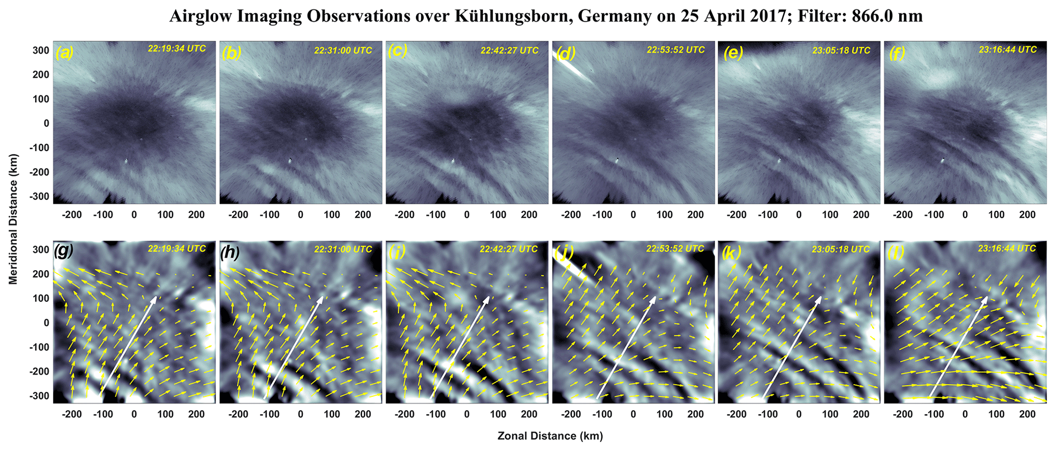
Figure 3 (a–f) Sequence of O₂ 866.0 nm airglow images on 25 April 2017 over northern Germany. (g–l) Corresponding 2D FFT filtered images overlaid on horizontal variation of wind field (yellow arrows) at the emission centroid height (94 km) measured by MMARIA. The white arrow denotes the wave vector.

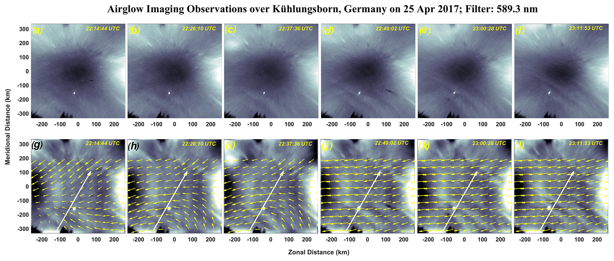
Figure 4 (a–f) Sequence of Na 589.3 nm airglow images on 25 April 2017 over northern Germany. (g–l) Corresponding 2D FFT filtered images overlaid on horizontal variation of wind field (yellow arrows) at the emission centroid height (91 km) measured by MMARIA. The white arrow denotes the wave vector.

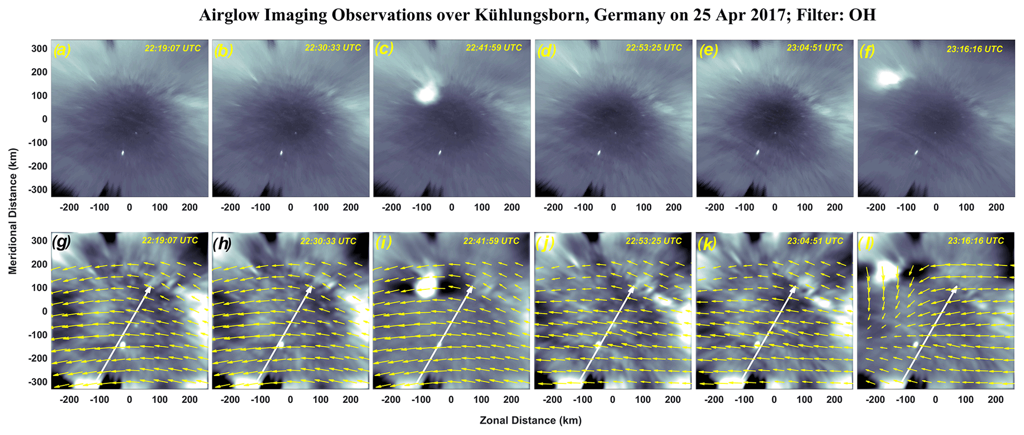
Figure 5 (a–f) Sequence of OH airglow images on 25 April 2017 over northern Germany. (g–l) Corresponding 2D FFT filtered images overlaid on horizontal variation of wind field (yellow arrows) at the emission centroid height (86 km) measured by MMARIA. The white arrow denotes the wave vector.

In order to investigate the vertical propagation characteristics of the observed wave structure through the OH, Na, O₂, and O(¹S) airglow emission layers, the altitude variation of squared vertical wavenumber (m²) needs to be computed. Following Nappo (2002), the relation for the vertical wavenumber can be expressed as

$$\begin{array}{}\text{(1)}& m^{\mathrm{2}}\left(z\right)={\displaystyle \frac{N^{\mathrm{2}}}{{\widehat{c}}^{\mathrm{2}}}}-{\displaystyle \frac{U_k^{\prime }}{H\widehat{c}}}-k_x^{\mathrm{2}}-{\displaystyle \frac{\mathrm{1}}{\mathrm{4}{H}^{\mathrm{2}}}}.\end{array}$$

Here, $k_x(\mathrm{2}\mathit{\pi }/{\mathit{\lambda }}_x)$ is the horizontal wavenumber (λ_x is the horizontal wavelength), H is the scale height, U_k is the projected wind along the wave vector, $U_k^{\prime }$ is the vertical wind shear, c is the observed phase velocity, and $\widehat{c}$ is the intrinsic phase velocity (c−U_k) are given. The values of H=5.4 km and k_x=0.084 km⁻¹ (λ_x=75 km). The altitude profile of the projected wind along the wave vector has been calculated from the altitude variation of the 2D horizontally resolved wind field within the observed structure. In addition, the 2D wind field at the centroid height of each airglow emission are overlaid on the filtered unwarped airglow images (shown in panels g–l of Figs. 2–5). This approach gives us the opportunity to calculate the horizontal wind velocity within the observed wave structure more precisely.

4 Results

Figures 2–5 depict all-sky airglow imaging observations at four different airglow emissions originating at the MLT region along with the MMARIA 2D horizontally resolved wind-field measurements over northern Germany during the cloudless and moonless night of 25 April 2017. Figure 2a–f show the sequence of unwarped images observed in O(¹S) airglow emission. The central dark spot appearing in every all-sky airglow image is due to the van Rhijn effect: a combination of the finite width of the emission layer and the variation of the line of sight through the layer with increasing zenith distance. Figure 2g–l depict the corresponding 2D FFT filtered images overlaid on the MMARIA horizontal 1 h averaged wind field in two dimensions at the centroid height of O(¹S) airglow emission in the MLT region. In a similar manner, the upper horizontal subplots in Figs. 2–4 represent the sequence of unwarped images observed in O₂, Na, and OH band emissions. The bottom subplots represent their corresponding 2D FFT filtered images overlaid on the MMARIA 2D horizontally resolved wind field at the centroid height of the respective airglow emissions. The winds are analyzed as an average along the propagation path of the wave fronts. The spatial wind retrievals imply a large spatial coherence of about 60 km (the correlation length is set to include the next grid cell) and a temporal correlation of about 30 min. Thus, a certain degree of coherence is an essential part of the wind analysis for this case. Furthermore, due to the thermal wind balance, changes in the vertical temperature profile led to corresponding changes of the winds at the different altitudes. The spatial variability of the wind field is also indicated by the bending of the wave fronts found in Figs. 2 and 3, whereas the wind fields remain stable at the altitude of the OH emission line presented in Fig. 5. We can observe the existence of a front-wall with small undulation wave structure in all the filters. The horizontal propagation of the observed wave structure is from southwest to northeast and entered within the FOV of the imager over northern Germany. The wave structure entered at the southwestern edge of the FOV of the imager at around 21:35 UT, although we have shown the sequence of images (Figs. 2–5) from 21:56 UT onward when the wave structure is fairly visible in the southwest corner of the imager FOV. The wave structure is very prominent in both O(¹S) and O₂ images. On the other hand, it is very faint in Na and OH images. It is interesting to note that the measurement location of SABER 2 falls in the path of the propagation of the wave structure.

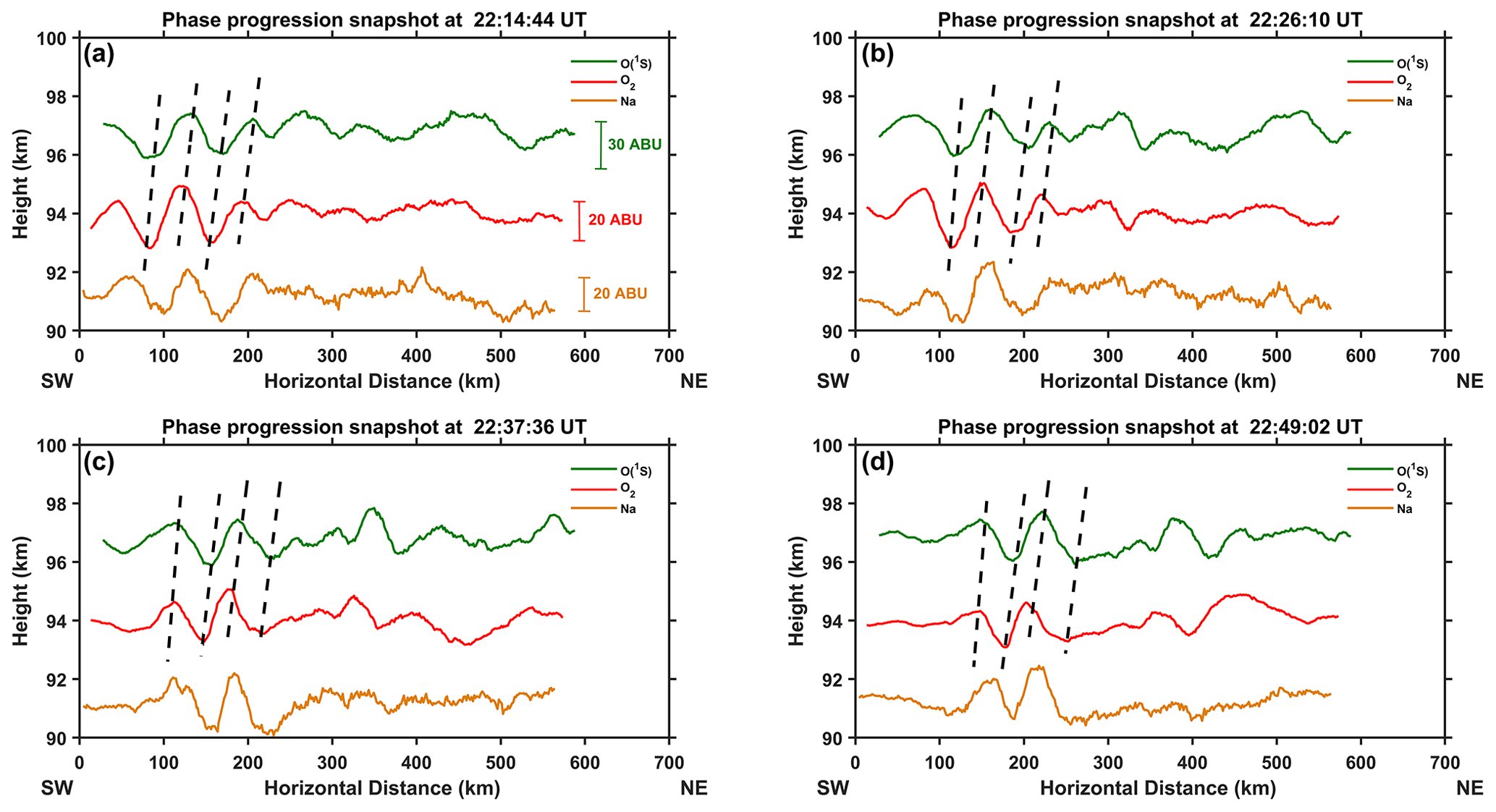
Figure 6 (a–d) The green, red, and orange solid lines in each panel depict the wind shear corrected intensity variation of O(¹S), O₂, and Na airglow emissions, respectively, along their line of propagation. The slices have also been horizontally shifted using the intrinsic horizontal wave speed in order to make a quasi-simultaneous “snapshot” of the vertical structure of the wave field. The slices have been separated vertically in order to represent the relative vertical separations of the emission layers in the MLT region. The emission brightness is given in arbitrary brightness units (ABU) in panel (a) and refers to all four panels.

In order to investigate the vertical phase propagation of the wave structure, the intensity of slices of O(¹S), O₂, and Na images were plotted at a given time in the direction of propagation, and they have been horizontally shifted based on its deduced phase speed of the leading front, to account for the acquisition time differences between each image. The observed mean phase velocities deduced from O(¹S), O₂, and Na images are 50.2 ± 4.8, 46.6 ± 4.2, and 44.5 ± 9.7 m s⁻¹, respectively. Since the wave structure appeared to be very faint in the OH images, observing the GWs in these images becomes practically impossible. A key element in the analyses is the horizontal vs. altitude intensity plot to determine the vertical phase propagation of the observed GW similar to Smith et al. (2005). The green, red, and orange lines in each subplot of Fig. 6a–d depict the intensity variation of O(¹S), O₂ and Na airglow emissions, respectively, along their line of propagation vector considering the large-scale vertical wind shear and thus obtaining the intrinsic phase progression, which is actually needed to distinguish the vertical propagation direction. The slices have been separated vertically in order to represent the assumed relative vertical separations of the emission layers in the MLT region corrected for the observed phase speed of the wave. We can clearly observe that the intrinsic phase in the O₂ airglow (centroid emission height: 94 km) is always lagging O(¹S) airglow (centroid emission height: 97 km). Thus, the lagging phase front in O₂ airglow, which is in the lower height, as compared to the O(¹S) airglow indicates that the phase front appeared in O(¹S) and then O₂ airglow emission layer. Therefore, the vertical phase progression of the wave structure is downward. Hence, based on this information, we can conclude that we have captured an event of an upward-propagating wave in O(¹S) and O₂ airglow emission layers on the night of 25 April 2017 over northern Germany. However, the intrinsic phase in the Na airglow (centroid emission height: 91 km) appears to lead the O₂ airglow, indicating that the vertical phase progression of the wave structure is different in the Na airglow emission layer as compared to O(¹S) and O₂ airglow emission layers. In addition, the Na airglow intensity variation also seems to be different at larger horizontal distances. However, we are unable find out the cause based on the present data set.

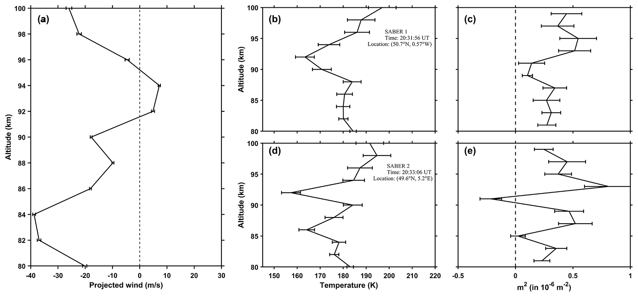
Figure 7 (a) The altitude profile of projected horizontal wind along the wave vector measured during 21:30–22:30 UT. (b–c) The altitude profiles of SABER temperature along with measurement uncertainty plotted as horizontal error bar over SABER 1 and 2 locations, respectively. (d–e) The altitude profiles of m² derived using the Eq. (1) along with the proportional error plotted as horizontal error bar over SABER 1 and 2 locations, respectively.

In order to find the vertical propagation characteristics of the wave structure, the derivation of the altitude profile of m² is required with the knowledge of the vertical temperature profiles and the projected wind along the wave vector. In addition, it is clear from Eq. (1) that we also need to calculate the intrinsic phase velocity of the wave structure. Hence, the horizontally spatially averaged projected wind profile within the region of wave structure and along the wave vector have been calculated and the hourly values for 21:30–22:30 UT are shown in Fig. 7a. Figure 7b and d depict the altitude profiles of SABER temperature along with the measurement uncertainty plotted as horizontal error bar over the SABER 1 and 2 locations (refer to Fig. 1), respectively. It is to be noted that the SABER temperature measurements were carried out around 1 h prior to the event. The change in the temperature within this short timescale is mainly due to wave perturbations, e.g., atmospheric tides. However, 1 h is still a short enough timescale to assume that the change in the background temperature is very small and, thus, is not going to affect the analyses. In addition, we did not observe any wave activities before and after the event. Hence, there will not be any significant differences in the temperature and this temperature profile has been used to calculate the altitude profile of m². Following Eq. (1) and based on the SABER temperature profile, imager, and MMARIA projected wind profile measurements, we have calculated the altitude profile of m². Figure 7c and e are the altitude profiles of m² along with the proportional error plotted as horizontal error bar over SABER 1 and 2 locations, respectively. Both m² profiles have been derived using the same projected wind shown in Fig. 7a. It is interesting to note that the temperature profile does not show any inversion at the SABER 1 location. However, we can observe the mesospheric inversion layer (MIL) at the SABER 2 location. The m² profile at SABER 2 reveals that a duct region exists in the altitude range between 85–91 km where positive m² is vertically sandwiched between a negative m² value (at 91 km) and a less positive value (at 85 km). In order to find the nature of the duct layer, we have analyzed the contribution of each term of the dispersion relation (Eq. 1). The contribution terms in m² profiles are like ∼ 89.5 % from the buoyancy term (thermal gradient) $\left(\frac{N^{\mathrm{2}}}{{\widehat{c}}^{\mathrm{2}}}\right)$, ∼ 6.5 % from the wind shear term $\left(\frac{U_k^{\prime }}{H\widehat{c}}\right)$, ∼ 1.9 % from squared of horizontal wavenumber k², and ∼ 2.1 % from scale height term $\left(\frac{\mathrm{1}}{\mathrm{4}{H}^{\mathrm{2}}}\right)$. The contribution suggests that the buoyancy term (thermal gradient) dominates in the m² profile, whereas the wind shear does not play any significant role. Therefore, the duct layer observed in the MIL region at 85–91 km is a thermal duct by nature, dominated by the thermal gradient of the MIL which is observed merely 1 h before the appearance of the wave fronts in the southwest region of imager FOV. It is worth mentioning that the observed MIL is close to the edge of the horizontal coverage of the airglow imager and coincide with the path of the propagation of the wave structure (refer to Figs. 2–5).

5 Discussion

As discussed above, the multiwavelength all-sky airglow imager installed at Kühlungsborn, Germany, can record images at four airglow emissions originating from the MLT region of the Earth's atmosphere. Our main objective is to combine data from the all-sky imager to investigate the spatial information of the waves in the MLT region and corroborate with the 2D horizontally resolved wind field at different altitudes using MMARIA. The optical and radio measurements in 2D give us a unique opportunity to investigate intriguing wave events in the MLT region over northern Germany. We have captured a front-like wave structure during the all-sky airglow imaging observation on 25 April 2017 at O(¹S), O₂, Na, and OH airglow emission layers. As discussed in the Results section, we captured an upward-propagating wave structure, and it appeared to be very prominent in both O(¹S) and O₂ images propagating from southwest to northeast. On the other hand, it is faintly observed in both Na and OH images. As the Na airglow is a relatively weaker emission compared to O(¹S) and O₂ airglow, it may be the plausible reason for observing faint structure in Na airglow images. Hence, it is expected that any wave structure observed in that filter may not be prominent due to poor signal-to-noise ratio. However, it is well-known that the OH airglow emission is much brighter than O₂ and O(¹S) emissions in the MLT region and has been widely used for the investigating of GWs (e.g., Taylor et al., 1995; Yamada et al., 2001; Mukherjee, 2003; Li et al., 2005; Yue et al., 2010). Hence, any wave structure should be very prominent in the OH airglow images. In fact, clear signatures of wave activities were observed on other nights in OH airglow images over northern Germany. However, the wave structure, on 25 April 2017, can barely be observed in the OH airglow images. The detailed analyses of the plausible cause behind the occurrence of this rare event have been carried out and discussed below.

5.1 Reduction in the OH airglow emission intensity

It is mentioned above that the OH airglow emission is normally a strong emission for the investigation of dynamics in the MLT region. However, reduction in the overall density of H atoms and O₃ molecules, which are reacting to form the excited OH molecule, could have led to the weak OH airglow emission on that night. Consequently, the wave structure observed in the OH filter may not appear as prominent as it should be, due to poor signal-to-noise ratio. In order to explore the possibilities, we have carried out comparison of the SABER measured altitude profiles of H atomic, O₃ molecular densities and OH volume emission rate (VER) profiles. The VER profiles (both at 1.6 and 2.0 µm emissions) at SABER 2 measurement location on the night of 25 April 2017 reveal that the thickness of the OH emission layer is ∼ 10.2 km. The SABER measurements indicated that the centroid height of OH airglow emission occurred near 87 km on that night. We have also looked into OH VER profiles for ±2 nights from nearby locations during 20:00–21:00 UT (figures not shown). We found that the OH emission layer thickness is similar (10.03 ± 0.6 km). Hence, we believe that the small changes in the thickness will not have any significant impact on the observability of the wave in OH airglow emission layer. In addition, we found that there are no significant differences of the density of H and O₃ and OH VER profiles. Hence, the fact that we observed the faint wave structure in the OH airglow image is not due to the reduction in the overall intensity level of OH airglow emission on that night.

5.2 Cancellation of waves in the OH airglow emission layer

Based on model calculation, Liu and Swenson (2003) reported that for vertically propagating GWs, the amplitude of airglow perturbations observed using ground-based measurements is larger for longer vertical wavelength, due to the smaller cancellation effect within each layer. This cancellation factor was introduced by Swenson and Gardner (1998) for OH airglow to relate the observed vertically integrated airglow intensity perturbations to the wave amplitudes. This cancellation factor causes a GW that may not be observable in an airglow emission layer, when observed using ground-based airglow instruments if the vertical wavelength is less than the FWHM (e.g., Swenson and Gardner, 1998; Liu and Swenson, 2003; Vargas et al., 2007).

Based on the sounding rocket measurements, it has been reported that the OH, Na, O₂, and O(¹S) airglow emission layers are originating in the MLT region with FWHM of 8–10 km (Watanabe et al., 1981; Ogawa et al., 1987; Baker and Stair, 1988; Gobbi et al., 1992; Hedin et al., 2009). On many occasions, these in situ rocket-borne measurements reveal that the FWHM of the O₂ emission layer is more than the one of OH, whereas the FWHM of Na airglow layer is nearly comparable with that of OH and O₂. However, in general, the FWHM of O(¹S) airglow layer is 1 or 2 km less compared to the OH and O₂ airglow emission layers. We have estimated the vertical wavelength of the wave structure from the phase shift of O₂ and O(¹S) airglow emission intensities (Fig. 6). From the slopes of the dashed lines, we can get the values of vertical wavelength ranging between 14 and 25 km. On the other hand, we can also calculate the average vertical wavelength using Eq. (1) (based on SABER and MMARIA measurements). It turns out to be 9.3 km in O₂ and O(¹S) airglow emission layers (Fig. 7e). The difference in the vertical wavelength calculated using two different methods is because of the two instruments that record different scale sizes due to differences in viewing geometries of each technique and the parameters recorded. In addition, from Fig. 7e, the average vertical wavelength of the wave structure is calculated to be 11.5 km (m² = 0.3 × 10⁻⁶ m²) in the OH airglow emission layer. Thus, it is clear that the vertical wavelength of the wave structure is longer than the OH emission layer thickness (10.2 km). Therefore, it is unlikely that the faint wave structure observed in the OH airglow images is due to the cancellation of waves in the OH airglow emission layer. It appears that this rare event occurred because of conducive background condition over northern Germany on that night.

5.3 Thermal ducting of waves

In order to investigate this interesting and intriguing observation, the derivation of the altitude profiles of m² has been carried out over both SABER 1 and 2 measurement locations. Figure 7 suggests the presence of a thermal duct layer (85–91 km) merely 1 h before the appearance of the wave fronts in the southwest region of imager FOV. It is well known that the MIL tends to be quite stable for at least 3–4 h (e.g., Dao et al., 1995; Meriwether and Gerrard, 2004). However, they can be spatially discontinuous as observed from SABER 1 and 2 temperature profiles. The theory of GW propagation predicts that the waves should reflect if the vertical wavenumber has an imaginary component. Hence, if m² < 0, then the transmitted wave will die out because of its amplitude decreases exponentially. It creates a region of evanescence in which the wave cannot vertically propagate and is reflected (Isler et al., 1997; Fritts and Yuan, 1989; Hines and Tarasick, 1994; Huang et al., 2010). In the present case, the wave structure freely propagated in three dimensions, and it encountered the bottom of the duct layer at 85 km. The m² profile indicates the existence of a weak evanescent region at 85 km. Therefore, the duct layer observed in the present case is a “leaky duct” from the bottom side. Thus, only a part of the wave energy could penetrate through the bottom of the duct layer. Thus, a few wave fronts traveling from southwest to northeast could partially enter from the bottom of the duct layer in the imager FOV in Na and OH airglow emission regime. The other part of the wave structure, which did not encounter the duct layer, freely propagated and entered in the FOV of the imager at O(¹S) and O₂ airglow emission layers situated at higher altitudes. This is supported by the phase progression analyses shown in Fig. 6, wherein we captured the wave structure as “upward-propagating wave” in O(¹S) and O₂ airglow emission layers on that night. However, the intrinsic phase of the wave structure in the Na airglow emission layer indicates that the vertical phase progression is different as compared to the O(¹S) and O₂ airglow emission layers. This difference in the vertical phase progression is caused by the combined effect of wave structure within and beyond the ducted layer as the airglow imager captured vertically integrated Na airglow emission intensity peaked at 91 km with a FWHM of ∼ 10 km (Mende et al., 1993). On the other hand, the intensity in the OH airglow images appeared so faint that the determination of the phase progression of the waves in these images becomes practically impossible. The multi-instrument observation gave us the opportunity to investigate the plausible physical process behind this intriguing and rare phenomenon where the thermally leaky ducted layer partially inhibited the wave progression in the OH airglow emission layer. As a result, the OH airglow images exhibit as the faint wave front on the night of 25 April 2017 over northern Germany.

It is to be noted that there is a lack of conclusive evidence for how the upward-propagating waves, which are detected in the O(¹S) and O₂ airglow emission layers, crossed the thermal duct to the southwest of Kühlungsborn. The waves would have to propagate nearly horizontally in order to reach the FOV of the imager at O(¹S) and O₂ airglow emission altitudes, which seems unlikely. However, if the thermal duct is highly localized over the SABER 2 location, it might be plausible that waves, which did not enter the duct layer, continued to propagate upward and were detected in O(¹S) and O₂ airglow emission layers. On the other hand, the ducted waves which have smaller amplitude propagated near horizontally towards the northeast direction in the OH and Na emission layers. The absence of coordinated temperature measurement over Kühlungsborn on that night keeps us from interpreting this observation conclusively.

6 Summary and conclusion

A case study of a wave event observed on the night of 25 April 2017 over northern Germany using optical and radar instruments is reported here. The multiwavelength all-sky airglow imager recorded an upward-propagating wave structure at multiple airglow altitudes in the MLT region. It appeared to be very prominent in O(¹S) and O₂ airglow images. However, the same wave structure is observed to be faint in both Na and OH airglow images, despite OH being one of the strong airglow emissions. In order to investigate this intriguing phenomenon, the derivation of the altitude profiles of m² was carried out using a colocated MMARIA altitude profile of the horizontally resolved wind field and a SABER temperature profile close to the event location. The obtained m² profiles indicates the presence of a thermal duct layer in the altitude range of 85–91 km in the southwest region of Kühlungsborn. The wave structure entered partially from the bottom of the leaky duct layer (at 85 km) and traveled from southwest to northeast (in the imager FOV) in the OH airglow emission layer, whereas the other part of the wave structure, which did not encounter the duct layer, freely propagated and entered the FOV of the imager at O(¹S) and O₂ airglow emission layers, resulting in the weak wave structure observed in the OH airglow images on that night over northern Germany.